Abstract
Accurately predicting the Remaining Useful Life (RUL) of milling tools based on monitoring signals is crucial for maximizing tool utilization and reducing machining costs. However, tool degradation and working conditions complicate the extraction of features from monitoring data, making the nonlinear mapping from these features to RUL challenging. To address this, a novel Kolmogorov–Arnold Attention Allocation Network (KA-AAN) is proposed, which consists of an Attentional Feature Extraction Network (AFEN) and a KAN regression block. First, the S-transform is applied to multi-sensor signals to create a time-frequency feature dataset. Then, the AFEN allocates attention to extracting attentional features concerning both tool degradation and working conditions by using multiple Kolmogorov–Arnold Attention Blocks and the unique activation function of KAN, which enhances the importance of features at different levels. Furthermore, the KAN regression block maps from attentional features to RUL, learning the most appropriate way to activate and combine features based on the specific circumstances of the tool and machining process. The nonlinear fusion of the attentional features improves the model’s adaptability to different working conditions. Finally, an experiment was designed and conducted to verify the robustness and stability of the proposed method. The experimental results show that the proposed method achieves a mean squared error of 0.97 and a mean absolute percentage error of 8.27% under the same working condition and 2.91% and 18.63% under different conditions (average). Compared to other advanced methods, the proposed method exhibits higher accuracy and adaptability.
1. Introduction
With the increasing demand for equipment and parts in aerospace, automotive, and precision machinery industries, tool wear has become a critical factor affecting productivity and product quality in modern manufacturing. Tool wear directly influences the surface quality of machined parts and can result in machine downtime, thereby escalating costs and diminishing production efficiency [1]. According to statistics, in April 2018, the cost of cutting tool scrap due to tool wear in the U.S. reached 200 million dollars [2]. Furthermore, approximately 20% of machine downtime is caused by tool failure [3]. Therefore, accurately predicting the Remaining Useful Life (RUL) of tools is essential for improving production efficiency, reducing tool waste, and cutting costs.
In recent years, machine learning and artificial intelligence have significantly advanced the development of RUL prediction models. Deep neural networks [4], Transformer networks [5], Long Short-Term Memory networks (LSTM) [6], Gated Recurrent Units [7], and Convolutional Neural Networks (CNN) [8] exhibit considerable potential in capturing both time and spatial features in machining data. However, these methods still face challenges in extracting nonlinear features during machining and managing data discrepancies arising from different working conditions. Feature extraction is central to artificial intelligence approaches [9]. Traditional methods depend on manually designed features, such as time-domain features (mean, standard deviation, skewness) and frequency-domain features (harmonic ratio, spectral amplitude, spectral density [10,11,12,13,14]). For instance, Wang and Azmi [15] used milling force signal features to describe tool wear conditions. Wei et al. [16] performed spectral analysis of milling forces and proposed a force signal decomposition model based on variational mode decomposition, which identified signal frequencies that reflect tool wear, avoiding mode mixing and improving tool condition monitoring. Wang et al. [3] constructed the total energy of the acoustic emission step signal as a feature and established the relationship between tool flank wear and the energy of acoustic emission signals, providing a new idea for manual feature extraction. Cho et al. [17] used the root mean square (RMS) value of acoustic emission signals to characterize the degradation of tool wear. Some researchers have attempted to use time-frequency features as input for AI methods to predict RUL [18]. For example, Ahsan et al. [19] used Short-Time Fourier Transform (STFT) to analyze bearing vibration signals, predicting RUL and fault types based on time-frequency similarity comparisons. Laddada et al. [20] developed a feature extraction method based on Continuous Wavelet Transform (CWT) and improved the extreme learning machine for RUL prediction. Chen et al. [21] employed statistical analysis, spectral analysis, and wavelet packet methods to detect tool wear during drilling. When obtaining the time-frequency features of milling, STFT [22] can effectively extract the time-frequency features of non-stationary signals. However, this method is limited by the Heisenberg uncertainty principle, which prevents it from simultaneously achieving high time and frequency resolution. CWT [23] has the advantage of variable window functions, providing much stronger resolution characteristics; however, the selection of its basis functions is relatively complex [24]. Empirical Mode Decomposition [25] overcomes the drawbacks of CWT and STFT by identifying vibration modes in the signal through time-scale features. It exhibits good adaptability; however, large oscillations can occur at the ends of the signal, potentially leading to instability in the intrinsic mode functions at the boundaries. To address these issues, Stockwell [26] proposed the S-Transform (ST), which combines the advantages of STFT and CWT. ST resolves the basis function selection issue of CWT and, using a scalable Gaussian window function, adjusts the window size and analysis range for different frequencies, offering both good time and frequency resolution. Although these methods are somewhat effective, they are inefficient, time-consuming, and heavily influenced by working conditions [27].
Some researchers have attempted to use time-frequency features as inputs for AI models to predict RUL. For example, Zhou et al. [28] pointed out that LSTM is advantageous in handling sensor time series and tool wear accumulation effects, but its feature extraction capability is weaker than that of CNN. Xu et al. [27] proposed a parallel CNN that implements multi-scale feature fusion and combines channel attention mechanisms with residual connections to improve RUL prediction performance. Li et al. [29] proposed a method for extracting multi-collinearity features from multi-sensor data and combining lightweight feature fusion methods with KPCA to remove redundant information, achieving accurate tool wear prediction. Feng et al. [24] used the Time–Space Attention (TSA) network, allowing different sensor signals to provide complementary information in the feature space. This enables more accurate capture of the complex spatiotemporal relationship between tool wear values and features, allowing the model to predict wear accurately even if cutting force signals with good trends are discarded. Li et al. [30] proposed a Convolutional Stacked Bidirectional LSTM Network with Time–Space Attention Mechanism (CSBLSTM-TSAM), which fuses multi-sensor signals to obtain tool wear values. Although these methods have improved efficiency and prediction accuracy, neural network-based feature extraction methods heavily depend on known data. When training samples fail to cover complex machining environments and diverse milling conditions, models tend to overfit working conditions.
Machine learning methods have made progress in RUL prediction for tools, but challenges remain as follows: (1) Insufficient prediction accuracy under different working conditions, especially when training data cannot cover complex environments. (2) Insufficient generalization of milling features due to the challenge of manually designed features being influenced by external disturbances. (3) Overfitting due to automatic feature learning, making the method unreliable for real-world applications. Therefore, there is an urgent need for a method that effectively integrates multi-sensor data and captures the complex relationships between RUL and features.
Kolmogorov–Arnold Networks (KAN) have gained significant attention in artificial intelligence for their robustness, scalability, and ability to handle high-dimensional data, making them ideal for various prediction tasks [31]. This paper proposes a novel Kolmogorov–Arnold attention allocation network (KA-AAN) to forecast milling tool RUL under different working conditions. Key contributions of the method include:
- (1)
- ST is applied to multi-sensor signals to extract time-frequency features, providing KA-AAN with as much processing information as possible, thereby avoiding overfitting caused by insufficient features and samples.
- (2)
- The Attentional Feature Extraction Network (AFEN) allocates attention to extracting attentional features concerning both tool degradation and working conditions, which effectively overcomes the problem of poor feature generalization in milling.
- (3)
- The KAN regression block maps from attentional features to RUL, learning the most appropriate way to activate and combine features based on the specific circumstances of the tool and machining process. The nonlinear fusion of the attentional features overcomes the problem of insufficient prediction accuracy of tool RUL under different working conditions.
KA-AAN effectively addresses the challenges of poor feature generalization and insufficient prediction accuracy under different working conditions. The remaining parts of this paper are structured as follows. Section 2 presents the problem definition. The structure and the mathematical principles of the proposed KA-AAN are elucidated in Section 3. The tool life test under different working conditions is designed to validate the proposed method in Section 4. Section 5 summarizes the conclusions of the paper.
2. Problem Definition
The essence of cutting tool RUL prediction based on multi-sensor monitoring signals is to establish the mapping relationship between the RUL T(t) and the feature vector X(t) of monitoring signals at processing time t. As shown in Figure 1, the modeling process can be expressed as follows:
where is an unknown nonlinear function, and represents random error. The accuracy of the prediction model depends on two factors: the quality of the extracted feature vector X(t) and the accuracy of the nonlinear mapping function . However, experiments show that different features of various monitoring signals exhibit discrepancies in the time-frequency domain, which poses a challenge in obtaining high-quality X(t). This variability is primarily due to the combined effects of sensor characteristics, changes in milling conditions, material property differences, and tool geometry.
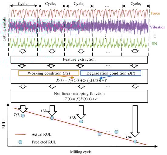
Figure 1.
Problem analysis based on a nonlinear mapping function.
By analyzing experimental data, the variation in the RMS features of the cutting force Fy in the feed direction and noise signals with milling time under the base condition is shown as the blue solid lines in Figure 2a,b. It is observed that as the milling cycles increase, the RMS features of both signals gradually increase. However, different working conditions have distinct impacts on the Fy and noise signal feature values and growth rate. From the frequency domain perspective, Figure 2c,d show the frequency domain plots of vibration signals at different times for the same tool. It can be observed that in the early stages of the tool’s life, frequency domain features are mainly reflected in the low-frequency components, while in the later stages, high-frequency components increase significantly [32]. Additionally, Figure 2e,f show the time-frequency plots of vibration signals after ST at different times for the same tool. It can be observed that the time-frequency features around 5 kHz increase significantly and become denser in the later stages of the tool’s life, while the features above 10 kHz also show an increase in amplitude but become sparser. In summary, the feature vector X(t)is not only influenced by the processing conditions C(t) (such as feed rate, cutting width, etc.) but also by the tool degradation state D(t) (such as wear level, crack formation, etc.). Therefore, X(t) can be viewed as a coupled function of processing conditions C(t) and degradation state D(t), which can be expressed as follows:
where fC(C(t)) is the influence function of C(t) on the features, representing the contribution of condition changes to the features; fD(D(t)) is the influence function of the degradation state D(t) on the features, representing the effect of tool degradation on the features; represents their nonlinear coupling, represents random error.
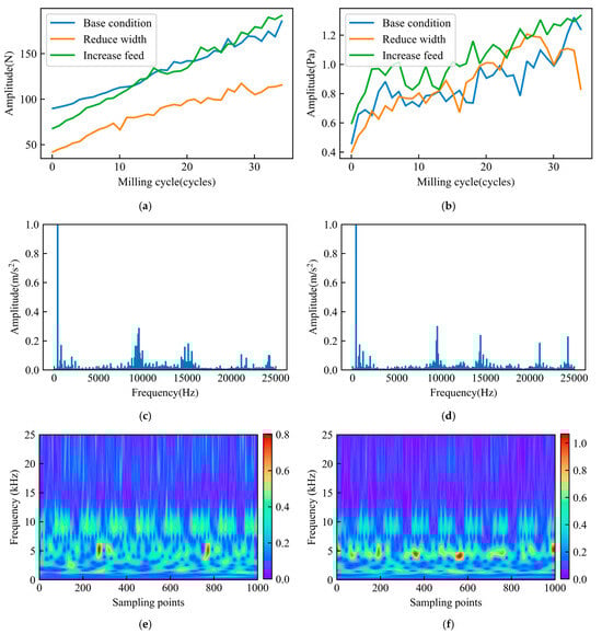
Figure 2.
Complex relationships in tool degradation data. (a) RMS of Fy under different working conditions; (b) RMS of noise under different working conditions; (c) Vibration spectrum of the 5th milling cycle; (d) Vibration spectrum of the 35th milling cycle; (e) Vibration time-frequency distribution figure of the 5th milling cycle; (f) Vibration time-frequency distribution figure of the 35th milling cycle.
The Traditional models, such as Multi-Layer Perceptron (MLP) and Recurrent Neural Networks (RNN), are limited by their fixed layers, nodes, and activation functions, restricting their ability to capture complex nonlinear relationships in different conditions of RUL prediction. Increasing the network depth and width can improve accuracy, but leads to computational overhead and overfitting. To overcome these limitations, this paper proposes a KA-AAN method for RUL prediction. AFEN is used to extract attentional features from the time-frequency domain that reflect both tool degradation and machining conditions, while KAN is used to fuse these attentional features and predict the RUL. KAN uses learnable B-spline curves to flexibly adapt to complex nonlinear relationships, enhancing its ability to capture intrinsic features of the data and effectively capture the complex nonlinear relationships between tool degradation and features. The RUL prediction model using KAN is expressed as:
where is a univariate activation function, q is the number of nodes in the previous layer, p is the number of nodes in the next layer, and the specific formula is in Section 3.2. By introducing learnable spline curves instead of fixed activation functions, KAN can achieve higher accuracy than MLP with fewer training iterations [33]. The problem in this paper can be transformed into extracting attentional features that reflect both tool degradation and machining conditions, and searching for the best activation function parameters to obtain the optimal mapping function .
3. Methodologies
This paper proposes a novel KA-AAN method for cutting tool RUL prediction, as shown in Figure 3. The method mainly consists of three stages: First, the raw signals are preprocessed by employing the ST on the multi-sensor machining data, constructing a time-frequency feature dataset that captures the tool’s machining process. Then, the Feature embedding and multiple KA-Attention Blocks are used in the AFEN to extract features and allocate importance to the time-frequency features, capturing the nonlinear mapping relationship between features and tool RUL, and obtaining attentional features. Finally, the KAN regression block maps from attentional features to RUL by using a learnable activation function. The features are activated and combined through a nonlinear function for predicting the tool’s RUL. The details of each stage are introduced as follows.
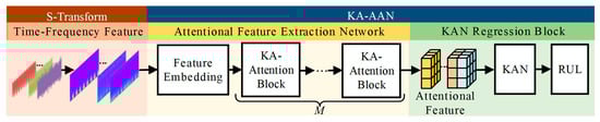
Figure 3.
General framework of the proposed method.
3.1. Time-Frequency Feature Based on S-Transform
Given the complexity of the time and frequency domains in the tool degradation process, this paper uses time-frequency features as input, applying the ST technique to transform the raw data and obtain time-frequency features for network input. The ST combines the advantages of STFT and CWT, allowing it to adaptively adjust the time-frequency resolution, overcoming the limitations of traditional methods. The one-dimensional continuous ST for the time-domain signal of the c-th sensor is defined as:
The inverse transformation of ST:
where f represents frequency, is the center point of the time window function, and t represents the time variable.
The wavelet function must satisfy the normalization condition:
Gaussian window function definition:
From the above, ST of uc(t) is defined as:
The discrete ST and its time-frequency complex matrix formula are:
In Equations (9) and (10), N is the number of sampling points and T is the sampling interval. Based on the above formulas, the window function of the ST has significant adaptive properties, and its variation amplitude decreases as the frequency increases. At this point, the magnitude of the time-frequency characteristic complex matrix obtained after discretizing the one-dimensional data from the c-th sensor through the ST is denoted as , and is used as the input to the proposed network.
3.2. Kolmogorov–Arnold Network
The Kolmogorov–Arnold network is a novel neural network inspired by the Kolmogorov–Arnold representation theorem [34]. The theorem states that any multivariable continuous function on a bounded domain can be represented as a finite combination of continuous functions of a single variable, along with binary addition operations. Inspired by this theorem, f(x) can be expressed as follows:
In Equation (11), the right side represents the KAN, where L denotes the number of layers, nj represents the number of nodes in the j-th layer, and is the single-variable activation function. As shown in Figure 4, each specific form defines the differences between various KAN architectures. In the initial implementation, is defined as a weighted combination of basic functions and B-splines. In particular,
where the basis function b(x) and the spline function spline(x) are defined as follows:
where , and are trainable parameters.
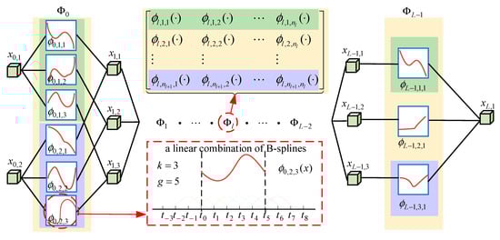
Figure 4.
Framework of KAN Layer.
The k-th order spline curve Bn(x) with grid size g is defined by the DeBoor-Cox recursive formula:
The pre-activation of is simply ; the post-activation of is denoted by . The activation value of the (l + 1, j) neuron is simply the sum of all incoming post-activations:
In matrix form, this reads as follows:
where is the function matrix corresponding to the lth KAN layer. A general KAN network is a composition of L layers: given an input vector , the output of KAN is as follows:
3.3. KA-AAN
The structure of the KA-AAN network is shown in Figure 5. AFEN consists of Feature embedding and M concatenated KA-Attention blocks. AFEN extracts features and allocates importance to the time-frequency features, obtaining attentional features. Finally, the KAN network fuses these attentional features to predict tool RUL. First, define the time-frequency feature matrix of the c-th sensor after the ST as Xc. The time-frequency feature matrices of all sensors are stacked to form a three-dimensional time-frequency feature matrix . The dimension of Xc is (F, R), where F is the number of frequency bins and R is the number of time steps. Feature embedding maps the raw data into fixed-size feature vectors for subsequent attention processing and computation:
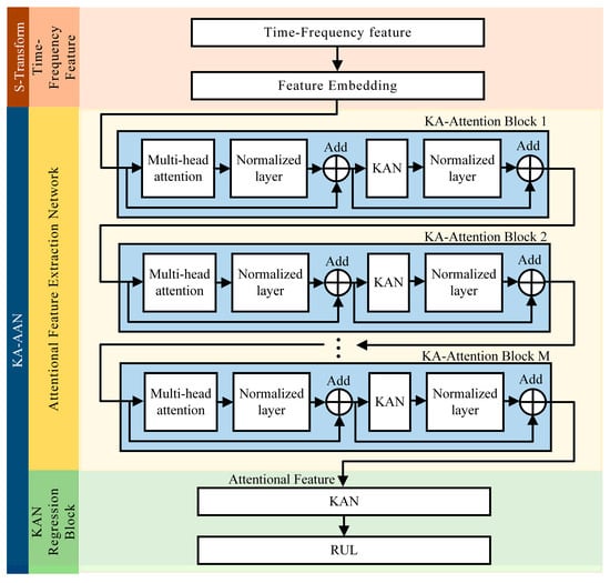
Figure 5.
The data flow of KA-AAN.
In the equation, is the feature matrix after Feature Embedding, W0 is the weight matrix, B0 is the bias matrix, with dimensions ,, , , and is the dimension of the embedded features.
The attention distribution for a single attention head first requires the computation of the Q, K, and V matrices:
In Equation (20), is the feature matrix after Feature Embedding, , , and are the mapping matrices, with dimensions , , and .
The attention is computed as follows:
Perform a multi-head attention operation on , where the multi-head attention model linearly maps Q, K, and V through projection matrices, then computes h attention scores, and finally concatenates the results. The computation for a single attention head is as follows:
In Equation (22), , , and are the Query, Key, and Value in the q-th self-attention mechanism, , , and are the mapping matrices for the q-th self-attention mechanism. The projection matrix projects Q, K, and V into h different attention heads to learn different attention patterns, improving model accuracy. Finally, the results of all attention heads are concatenated.
In Equation (23), Concat represents the matrix concatenation function. is the linear mapping matrix for concatenation.
To accelerate network convergence and improve generalization, layer normalization is applied to each sub-layer:
In Equation (24), LayerNorm(u) is the output of layer normalization; and are the scaling parameters; and are the mean and standard deviation of u.
The outputs of M layers of KA-Attention blocks are concatenated to form the tool health state attentional feature:
In Equation (25), is the feature matrix after Feature Embedding, F represents the network consisting of M-layer KA-Attention blocks, represents the internal parameters of the M-layer KA-Attention blocks, and represents the matrix concatenation function. Input g into the KAN network described in Section 3.2 for nonlinear regression, as shown below:
In Equation (26), KAN represents the nonlinear mapping function from the tool attentional feature g to the tool RUL, with being the internal parameters of KAN.
4. Experimental Setup and Prediction Results
4.1. Experimental Setup
The proposed method was validated using milling tool life test data. The experiment was conducted on a DX650 CNC machine, with a schematic of the test platform shown in Figure 6a. The platform is equipped with 7 sensors: one three-axis accelerometer, three uniaxial accelerometers, one three-axis force sensor, one microphone, and one acoustic emission sensor, yielding a total of 11 data channels. The sensor layout is shown in Figure 6b. The specific milling tool type and sensor manufacturers and types are listed in Table 1.
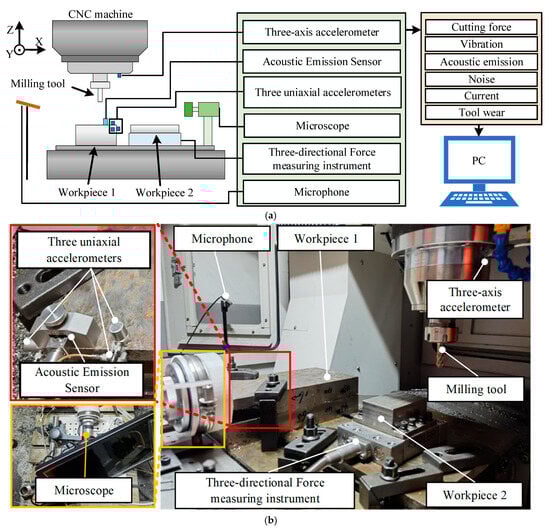
Figure 6.
Milling tool life test platform and measurement point arrangement. (a) Milling tool life test schematic; (b) Measurement point arrangement.

Table 1.
Milling tool and sensor types.
The workpiece material and working conditions were set based on engineering practice, as detailed in Table 2. The wear degradation trajectory of the tool is shown in Figure 7. As the milling cycles increase, the wear width increases accordingly. According to the tool failure criterion in ISO 8688-2, the tool is considered failed when the flank wear exceeds 300 μm, at which point the test is terminated. The ISO standard [35] specifies a 25 mm diameter end mill, different from the 10 mm diameter tool used in this experiment. The failure threshold for this test was set at 110 μm based on the onset of red-hot tool edges and significant sparking.
Table 2.
Milling experimental parameters setup for working conditions.
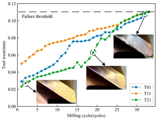
Figure 7.
Wear measurement results of T01, T11, and T21.
The ST is shown to be effective in processing machining signals. On the one hand, ST offers higher time resolution for high-frequency signals, and on the other, it maintains a lower amplitude and correlation for low-frequency signals. Figure 8 compares the time-domain signals and their time-frequency representations for the Y-direction milling force (Fy) and Y-axis spindle vibration signal (VSy) during the 1st and 35th milling cycles. The milling force is concentrated in the low-frequency range, with minimal noise. As the milling cycles increase, the amplitude gradually rises, and the red regions in the time-frequency signals intensify. Conversely, the high-frequency portion of the spindle vibration signal becomes sparse with the increasing number of cycles, while the low-frequency part gradually increases in amplitude.
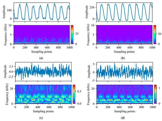
Figure 8.
S-transformation of partially processed signals. (a) Fy time-frequency distribution figure of the 1st milling cycle; (b) Fy time-frequency distribution figure of the 35th milling cycle; (c) VSy time-frequency distribution figure of the 1st milling cycle; (d) VSy time-frequency distribution figure of the 35th milling cycle.
Seven comparative experiments were conducted using the training and testing configurations shown in Table 3, with hyperparameters set in Table 4. The aim is to evaluate the method’s adaptability to both same-condition and different-condition scenarios. Case 0 primarily tests the prediction accuracy of the proposed method under the assumption of sufficient known information. Cases 1, 2, and 3 focus on training and testing under the same conditions. Cases 4, 5, and 6 evaluate the proposed network’s prediction accuracy and adaptability to unknown conditions.
Table 3.
Configuration of training and testing samples.
Table 4.
Hyper Parameter Setting.
4.2. Results and Discussions
In order to quantitatively and comprehensively evaluate the performance of the model, the MAPE, the MSE, the RMSE, and the coefficient of determination R2 are used as evaluation metrics. The calculation formulas of each metric are as follows:
where denotes the c-th predicted value, denotes the c-th actual value, and denotes the sample mean.
To validate the effectiveness of the proposed method, this paper compares several commonly used and advanced prediction models, including CNN, CNN-Bi-LSTM, Time–Space Attention (TSA) [24], and CSBLSTM-TSAM [30]. In Case 0, an 8:2 random training-test split, the proposed method achieved a MAPE of 8.01%, the best among all metrics. In the same condition cases (1, 2, and 3), CNN and CNN-Bi-LSTM had MAPE values of 19.47% and 30.28%, respectively. Bi-LSTM struggled to capture nonlinear patterns, which hurt its prediction accuracy. TSA and CSBLSTM-TSAM showed stable performance, with TSA slightly less accurate than CSBLSTM-TSAM. The proposed method significantly improved prediction accuracy, reducing RMSE and MAPE by 41.04% and 49.29% compared to TSA, and 27.57% and 29.76% compared to CSBLSTM-TSAM. As shown in Figure 9, the proposed method effectively captures tool degradation patterns under the same conditions and rich historical data, offering superior RUL prediction accuracy.
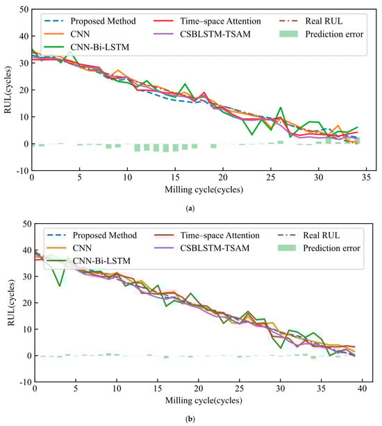
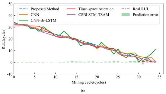
Figure 9.
RUL results were estimated using the proposed method and comparison methods under the same working conditions. (a) Case 1; (b) Case 2; (c) Case 3.
The prediction results for Cases 4–6 under multi-condition scenarios are shown in Figure 10. In the MSE comparison, KA-AAN had the lowest MSE (2.9148, average results of Cases 4–6), outperforming CNN (23.9993), CNN-Bi-LSTM (23.5929), TSA (10.0663), and CSBLSTM-TSAM (7.9647). This shows that the proposed method has the smallest prediction bias. The proposed method achieved the best results in R2, MAPE, and RMSE. It reduced RMSE and MAPE by 3.8756 and 38.71%, respectively, compared to CNN.
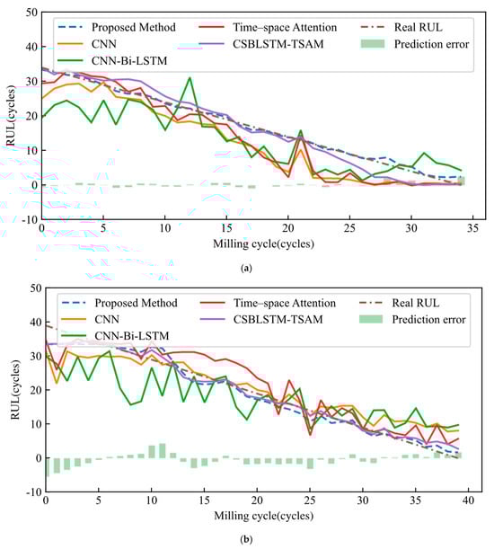
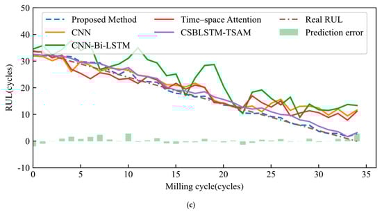
Figure 10.
RUL results were estimated using the proposed method and comparison methods under different operation conditions. (a) Case 4; (b) Case 5; (c) Case 6.
The average MAPE of KA-AAN is about 20% lower than that of TSA and 18% lower than that of CSBLSTM-TSAM. The RUL prediction results using the five models for Cases 4, 5, and 6 are shown in Figure 10a–c. The results show that KA-AAN more effectively captures tool degradation patterns and has a clear advantage in RUL prediction. In contrast, CNN and CNN-Bi-LSTM show large errors and fluctuations in early predictions. TSA, CSBLSTM-TSAM, and the proposed method follow prediction trends closer to the actual RUL. However, TSA shows a deviation in the later stages of prediction. In Case 4, the deviation is near 0, but in Cases 5 and 6, it diverges from the true value.
The evaluation metrics for the same condition and different condition cases under the five methods are shown in Figure 11a,b. The bar heights for CNN and CNN-Bi-LSTM are significantly higher, indicating larger prediction errors. The bars for TSA and CSBLSTM-TSAM are close in their respective ranges, but the bars for the proposed method are noticeably lower, showing smaller errors. In Figure 11a, the proposed method shows generally better MAPE, especially in Case 2, with an MAPE of 4.01%, showing significant improvement. The proposed method has the lowest average MAPE of 8.27% (average results of Cases 1–3), compared to other models. In Figure 11b, the proposed method’s MAPE (18.63%, average results of Cases 4–6) is still the lowest. Although the error in Case 6 is larger, it still outperforms the other models.
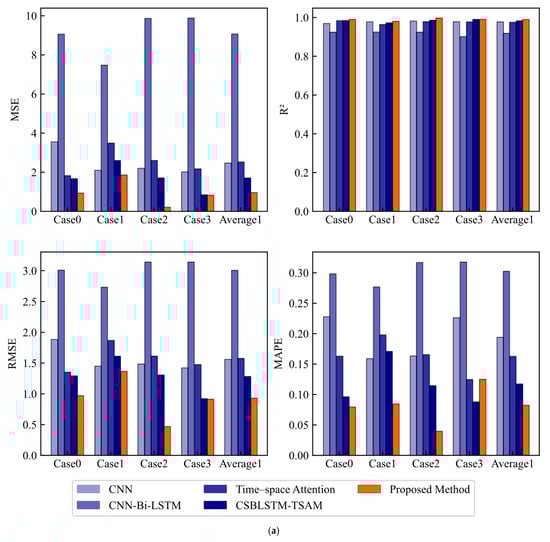
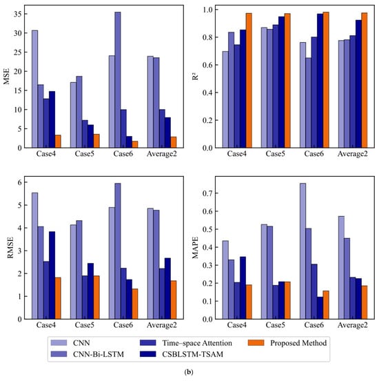
Figure 11.
Comparison of predictive performance. (a) Prediction performance under the same working conditions; (b) Prediction performance under different working conditions.
Notably, under the same condition scenarios, the R2 of CNN, CNN-Bi-LSTM, TSA, and CSBLSTM-TSAM are only slightly lower than that of the proposed method, still showing strong predictive ability. However, under different condition scenarios, the R2 of CNN, CNN-Bi-LSTM, and TSA significantly decreased, by 20.5%, 14.9%, and 16.7%, respectively, compared to the same condition cases. CSBLSTM-TSAM saw a smaller decrease of just 6.1%, showing better adaptability to different condition scenarios. The proposed method’s R2 decreased by only 1.4% under different condition scenarios, showing the best stability and predictive performance. Overall, the proposed method maintains higher stability and superior performance in different condition scenarios, especially in complex environments.
5. Conclusions
This paper proposes a novel KA-AAN for cutting tool RUL prediction. The method first employs ST to convert the multi-sensor signals from the machining process into time-frequency features. Then, AFEN allocates importance to these features to obtain attentional features, which are ultimately used in the KAN network for tool RUL prediction. The performance of the proposed method is validated through cutting tool life milling experiments, leading to the following conclusions:
- (1)
- The innovative use of AFEN in the method allocates importance to the features in the time-frequency domain. This captures the complex nonlinear mapping relationship between time-frequency features and RUL, effectively overcoming the problem of the limited generalization ability of milling features.
- (2)
- KAN is used to fuse the attentional features after attention redistribution. By replacing the traditional activation function with a learnable spline curve and optimizing the weight parameters of the spline curve, the nonlinear relationship between the signal features and tool RUL is accurately captured, enabling precise prediction of tool RUL under different working conditions.
- (3)
- RUL prediction experiments conducted using the milling tool life dataset validate the effectiveness of the method. Comparative analysis shows that the errors associated with the proposed method are relatively small, with the MSE and MAPE between predicted RUL and actual RUL reaching 2.91 and 18.63%, respectively. The average MAPE of KA-AAN is about 20% lower than that of Time–Space Attention and about 18% lower than CSBLSTM-TSAM (Notes: The performance metrics reported in the abstract and conclusion for ‘same working conditions’ and ‘different working conditions’ represent the average results over Cases 1–3 and Cases 4–6, respectively. Case 0, in contrast, evaluates model performance under a random train-test split across the entire dataset, regardless of operating conditions.
In future work, the method will be further tested under more diverse cutting conditions. We will also analyze the solvability of the KA-AAN network. Additionally, the KAN network will be optimized and pruned. We aim to explore the possibility of converting the prediction model into a specific formula. Finally, we will work on enhancing the interpretability of the tool for RUL prediction.
Author Contributions
Validation, L.S.; Writing—original draft, Y.L.; Writing—review and editing, D.G.; Funding acquisition, G.L. All authors have read and agreed to the published version of the manuscript.
Funding
National Natural Science Foundation of China (No.62203193) and Jiangsu Province Higher Education Institutions Basic Disciplines (21KJB510016).
Institutional Review Board Statement
Not applicable.
Informed Consent Statement
Not applicable.
Data Availability Statement
The data presented in this study are available in the article.
Conflicts of Interest
The authors declare no conflicts of interest.
References
- Zhu, K.; Zhang, Y. A generic tool wear model and its application to force modeling and wear monitoring in high speed milling. Mech. Syst. Signal Process. 2019, 115, 147–161. [Google Scholar] [CrossRef]
- Li, Z.; Liu, R.; Wu, D. Data-driven smart manufacturing: Tool wear monitoring with audio signals and machine learning. J. Manuf. Process. 2019, 48, 66–76. [Google Scholar] [CrossRef]
- Wang, C.; Bao, Z.; Zhang, P.; Ming, W.; Chen, M. Tool wear evaluation under minimum quantity lubrication by clustering energy of acoustic emission burst signals. Measurement 2019, 138, 256–265. [Google Scholar] [CrossRef]
- Deutsch, J.; He, D. Using Deep Learning-Based Approach to Predict Remaining Useful Life of Rotating Components. IEEE Trans. Syst. Man Cybern. Syst. 2018, 48, 11–20. [Google Scholar] [CrossRef]
- Mo, Y.; Wu, Q.; Li, X.; Huang, B. Remaining useful life estimation via transformer encoder enhanced by a gated convolutional unit. J. Intell. Manuf. 2021, 32, 1997–2006. [Google Scholar] [CrossRef]
- Yousuf, S.; Khan, S.A.; Khursheed, S. Remaining useful life (RUL) regression using Long–Short Term Memory (LSTM) networks. Microelectron. Reliab. 2022, 139, 114772. [Google Scholar] [CrossRef]
- Cao, L.; Zhang, H.; Meng, Z.; Wang, X. A parallel GRU with dual-stage attention mechanism model integrating uncertainty quantification for probabilistic RUL prediction of wind turbine bearings. Reliab. Eng. Syst. Saf. 2023, 235, 109197. [Google Scholar] [CrossRef]
- Zhang, X.; Shi, B.; Feng, B.; Liu, L.; Gao, Z. A hybrid method for cutting tool RUL prediction based on CNN and multistage wiener process using small sample data. Measurement 2023, 213, 112739. [Google Scholar] [CrossRef]
- Zhao, R.; Yan, R.; Chen, Z.; Mao, K.; Wang, P.; Gao, R.X. Deep learning and its applications to machine health monitoring. Mech. Syst. Signal Process. 2019, 115, 213–237. [Google Scholar] [CrossRef]
- Li, G.; Xu, S.; Jiang, R.; Liu, Y.; Zhang, L.; Zheng, H.; Sun, L.; Sun, Y. Physics-informed inhomogeneous wear identification of end mills by online monitoring data. J. Manuf. Process. 2024, 132, 759–771. [Google Scholar] [CrossRef]
- Nasir, V.; Dibaji, S.; Alaswad, K.; Cool, J. Tool wear monitoring by ensemble learning and sensor fusion using power, sound, vibration, and AE signals. Manuf. Lett. 2021, 30, 32–38. [Google Scholar] [CrossRef]
- Li, G.; Shang, X.; Yang, L.; Xie, D.; Sun, L.; Si, M.; Zhou, H. Milling tool wear condition monitoring based on physics-informed autoregression transformation of audio signals. IEEE Sensors J. 2025. [Google Scholar] [CrossRef]
- Cao, X.-C.; Chen, B.-Q.; Yao, B.; He, W.-P. Combining translation-invariant wavelet frames and convolutional neural network for intelligent tool wear state identification. Comput. Ind. 2019, 106, 71–84. [Google Scholar] [CrossRef]
- Chen, Y.; Jin, Y.; Jiri, G. Predicting tool wear with multi-sensor data using deep belief networks. Int. J. Adv. Manuf. Technol. 2018, 99, 1917–1926. [Google Scholar] [CrossRef]
- Azmi, A.I. Monitoring of tool wear using measured machining forces and neuro-fuzzy modelling approaches during machining of GFRP composites. Adv. Eng. Softw. 2015, 82, 53–64. [Google Scholar] [CrossRef]
- Wei, X.; Liu, X.; Yue, C.; Wang, L.; Liang, S.Y.; Qin, Y. Tool wear state recognition based on feature selection method with whitening variational mode decomposition. Robot. Comput.-Integr. Manuf. 2022, 77, 102344. [Google Scholar] [CrossRef]
- Cho, S.; Binsaeid, S.; Asfour, S. Design of multisensor fusion-based tool condition monitoring system in end milling. Int. J. Adv. Manuf. Technol. 2010, 46, 681–694. [Google Scholar] [CrossRef]
- Zhang, X.; Lu, X.; Li, W.; Wang, S. Prediction of the remaining useful life of cutting tool using the hurst exponent and CNN-LSTM. Int. J. Adv. Manuf. Technol. 2021, 112, 2277–2299. [Google Scholar] [CrossRef]
- Ahsan, M.; Salah, M.M. Similarity index of the STFT-based health diagnosis of variable speed rotating machines. Intell. Syst. Appl. 2023, 20, 200270. [Google Scholar] [CrossRef]
- Laddada, S.; Si-Chaib, M.O.; Benkedjouh, T.; Drai, R. Tool wear condition monitoring based on wavelet transform and improved extreme learning machine. Proc. Inst. Mech. Eng. Part C J. Mech. Eng. Sci. 2020, 234, 1057–1068. [Google Scholar] [CrossRef]
- Chen, X.; Li, B. Acoustic emission method for tool condition monitoring based on wavelet analysis. Int. J. Adv. Manuf. Technol. 2007, 33, 968–976. [Google Scholar] [CrossRef]
- Mustafa, D.; Yicheng, Z.; Minjie, G.; Jonas, H.; Jürgen, F. Motor current based misalignment diagnosis on linear axes with short-time fourier transform (STFT). Procedia CIRP 2022, 106, 239–243. [Google Scholar] [CrossRef]
- Yang, Q.; Tang, B.; Deng, L.; Zhu, P.; Ming, Z. WTFormer: RUL prediction method guided by trainable wavelet transform embedding and lagged penalty loss. Adv. Eng. Inform. 2024, 62, 102710. [Google Scholar] [CrossRef]
- Feng, T.; Guo, L.; Gao, H.; Chen, T.; Yu, Y.; Li, C. A new time–space attention mechanism driven multi-feature fusion method for tool wear monitoring. Int. J. Adv. Manuf. Technol. 2022, 120, 5633–5648. [Google Scholar] [CrossRef]
- Guo, X.; Wang, K.; Yao, S.; Fu, G.; Ning, Y. RUL prediction of lithium ion battery based on CEEMDAN-CNN BiLSTM model. Energy Rep. 2023, 9, 1299–1306. [Google Scholar] [CrossRef]
- Stockwell, R.G.; Mansinha, L.; Lowe, R.P. Localization of the complex spectrum: The S transform. IEEE Trans. Signal Process. 1996, 44, 998–1001. [Google Scholar] [CrossRef]
- Xu, X.; Wang, J.; Zhong, B.; Ming, W.; Chen, M. Deep learning-based tool wear prediction and its application for machining process using multi-scale feature fusion and channel attention mechanism. Measurement 2021, 177, 109254. [Google Scholar] [CrossRef]
- Zhou, J.-T.; Zhao, X.; Gao, J. Tool remaining useful life prediction method based on LSTM under variable working conditions. Int. J. Adv. Manuf. Technol. 2019, 104, 4715–4726. [Google Scholar] [CrossRef]
- Li, Y.; Wang, X.; He, Y.; Wang, Y.; Wang, S.; Wang, S. Deep spatial-temporal feature extraction and lightweight feature fusion for tool condition monitoring. IEEE Trans. Ind. Electron. 2022, 69, 7349–7359. [Google Scholar] [CrossRef]
- Li, X.; Liu, X.; Yue, C.; Wang, L.; Liang, S.Y. Data-model linkage prediction of tool remaining useful life based on deep feature fusion and wiener process. J. Manuf. Syst. 2024, 73, 19–38. [Google Scholar] [CrossRef]
- Schmidt-Hieber, J. The kolmogorov–arnold representation theorem revisited. Neural Netw. 2021, 137, 119–126. [Google Scholar] [CrossRef] [PubMed]
- Guo, H.; Zhang, Y.; Zhu, K. Interpretable deep learning approach for tool wear monitoring in high-speed milling. Comput. Ind. 2022, 138, 103638. [Google Scholar] [CrossRef]
- Liu, Z.; Ma, P.; Wang, Y.; Matusik, W.; Tegmark, M. KAN 2.0: Kolmogorov-arnold networks meet science. arXiv 2024, arXiv:2408.10205. [Google Scholar] [CrossRef]
- Liu, Z.; Wang, Y.; Vaidya, S.; Ruehle, F.; Halverson, J.; Soljačić, M.; Hou, T.Y.; Tegmark, M. KAN: Kolmogorov-arnold networks. arXiv 2024, arXiv:2404.19756. Available online: http://arxiv.org/abs/2404.19756 (accessed on 1 October 2025).
- ISO 8688-2; Tool Life Testing in Milling; Part 2: End Milling. ISO: Vernier, Geneva, 1989.


Disclaimer/Publisher’s Note: The statements, opinions and data contained in all publications are solely those of the individual author(s) and contributor(s) and not of MDPI and/or the editor(s). MDPI and/or the editor(s) disclaim responsibility for any injury to people or property resulting from any ideas, methods, instructions or products referred to in the content. |
© 2025 by the authors. Licensee MDPI, Basel, Switzerland. This article is an open access article distributed under the terms and conditions of the Creative Commons Attribution (CC BY) license (https://creativecommons.org/licenses/by/4.0/).