Abstract
This study investigates the spatial distribution of the hydromagnesite (HM) mineral in Akgöl, a closed basin located in the arid southwestern region of Türkiye, through the integration of geochemical analyses and remote sensing techniques. A total of 70 sediment samples were analyzed using X-ray Fluorescence (XRF), X-ray Diffraction (XRD), and spectroradiometry to determine their mineralogical composition. The resulting data were integrated with ASTER satellite imagery, and mineral distribution maps were generated across 13,293 pixels using multiple linear regression and Kriging interpolation techniques within the ArcGIS environment. The findings indicate that hydromagnesite is predominantly concentrated in the central part of the lake, where it represents the dominant mineral phase in contrast to lower concentrations observed along the periphery. The endorheic nature of Akgöl is comparable to other saline lakes with similar geological and climatic settings, such as Salda and Acıgöl, supporting the applicability of this methodological approach to mineral exploration in other arid and semi-arid environments. The study contributes not only to the regional assessment of mineral potential but also to the advancement of remote sensing and GIS-based analytical methods in geoscientific research.
1. Introduction
Geochemical mapping constitutes a comprehensive methodological framework aimed at systematically analyzing and spatially visualizing the chemical composition and mineralogical characteristics of the Earth’s surface materials. This technique plays a pivotal role in a wide array of geoscientific and environmental applications, including soil fertility assessments, environmental monitoring, and the interpretation of geological structures [1,2]. Through detailed analysis of elemental concentrations in soil, rock, and water samples, geochemical mapping enables the differentiation of natural and anthropogenic influences, thereby facilitating the development of targeted and evidence-based management strategies [3,4].
The outputs of geochemical mapping—primarily in the form of spatial distribution maps—are not merely descriptive but also serve predictive and diagnostic functions within decision-support systems. In mineral exploration, such maps are indispensable for delineating prospective zones, refining exploration models, and optimizing field operations. Furthermore, in environmental geochemistry, geochemical maps inform risk assessments by identifying pollutant dispersion patterns, delineating contamination hotspots, and guiding remediation efforts. Given these multifaceted applications, geochemical mapping stands as a foundational tool in interdisciplinary domains spanning geology, environmental science, natural resource management, and land-use planning [5,6].
In recent years, the integration of advanced analytical technologies into geochemical investigations has become increasingly prevalent, particularly in efforts to enhance the spatial resolution and accuracy of geochemical distribution analyses. Among these, X-ray fluorescence (XRF) and X-ray diffraction (XRD) techniques have emerged as pivotal tools, offering high precision in the characterization of both elemental compositions and mineralogical structures [7,8]. XRF is widely recognized for its rapid throughput and cost-effectiveness, making it ideal for quantifying elemental concentrations across large sample sets. Conversely, XRD provides critical insights into mineralogical and crystallographic properties, playing an essential role in the identification of mineral phases at or near the Earth’s surface [7,8]. When employed in tandem, these complementary techniques offer a robust analytical framework that enhances the interpretability of geological processes and environmental patterns through integrated, high-resolution data outputs.
The combined application of X-ray fluorescence (XRF) and X-ray diffraction (XRD) techniques offers significant advantages in the analysis of large geochemical datasets, particularly by enhancing the ability to characterize spatial heterogeneity in environmental and subsurface systems [7,9]. This integrative approach not only strengthens data acquisition but also deepens interpretive capacity by enabling the generation of more accurate geospatial models of elemental distributions and mineral phases. Within this context, geochemical mapping has proven to be an effective tool for delineating mineral distributions, tracking the dispersion of environmental contaminants, and identifying factors that influence agricultural productivity [7]. The complementary nature of XRF and XRD renders their combined use a robust methodological framework for spatial analysis, facilitating high-resolution, multi-dimensional interpretations across diverse geoscientific domains. Accordingly, this synergy contributes substantially to both geological investigations and interdisciplinary environmental studies by supporting comprehensive, reliable, and scalable data interpretations [7,9].
Multiple regression analysis has proven to be a powerful statistical tool, particularly effective in modeling the complex and often non-linear relationships among geochemical parameters. By capturing these intricate interactions, the method enhances the spatial accuracy of environmental and geological datasets, thereby supporting evidence-based decision-making in field applications [10,11,12]. Geographic Information Systems (GIS), especially platforms like ArcGIS, offer a robust analytical environment for the processing, visualization, and spatial interpretation of such multivariate models. These systems enable dynamic examination of spatial distributions, facilitating a deeper understanding of environmental system behaviors and spatial variability [13,14]. Furthermore, regression-based interpolation maps derived from these analyses provide a nuanced representation of regional heterogeneity, allowing for more precise spatial delineation and serving as strategic tools in local-scale planning and environmental assessment [13].
Hydromagnesite (HM) is a naturally occurring carbonate mineral characterized by its high magnesium content and widespread global distribution [15]. Its chemical formula, Mg5(CO3)4(OH)2·4H2O, corresponds to a theoretical composition of approximately 42.92% MgO, 37.77% CO2, and 19.31% H2O, with minor impurities such as SiO2, CaO, Fe2O3, and Al2O3 commonly present in trace amounts [16]. With a molecular weight of about 365.31 g/mol and a Mohs hardness of 3.5, HM is considered a moderately hard mineral [17].
Morphologically, HM typically appears as a fine-grained, greyish-white mineral exhibiting a microcrystalline texture, and is often found in powdery to massive forms. It frequently displays characteristic laminated and porous surface morphologies [18,19]. The presence of hydroxyl groups within its crystal structure confirms its hydrated nature, a trait that significantly influences its spectral behavior—especially in the context of remote sensing applications. In the electromagnetic spectrum, Visible and Near-Infrared (VNIR) bands reflect electronic transitions associated with specific metal ions, whereas Short-Wave Infrared (SWIR) bands are sensitive to the vibrational modes of hydroxyl groups. Additionally, Thermal Infrared (TIR) regions can detect radical vibrational frequencies, making it possible to distinguish HM from anhydrous and non-hydroxylated minerals [20].
Thanks to its unique physical and chemical characteristics, hydromagnesite is widely utilized across multiple industrial sectors, including chemical manufacturing, pharmaceuticals, construction materials, and electronics, highlighting its economic and strategic significance [21].
At present, significant hydromagnesite (HM) mineral deposits have been identified in several countries, including Canada, Türkiye, Greece, the United States, the United Kingdom, Spain, and China. The mineral was first described in Canada in 1915 and was reported as a soft white carbonate mineral [22,23]. Large-scale HM accumulations have since been discovered in salt lake environments such as Meadow, Cariboo, and Alberto [24]. Subsequent discoveries in southwestern Türkiye (Burdur) [25], the Salda region near Tuz Lake, and northern Greece [26] revealed additional extensive deposits, which are currently being exploited through industrial-scale operations [23].
Beyond these regions, other notable occurrences have been documented in Salzburg (Austria), Soghan (Iran), Carlsbad (CA, USA), the Pennine region (UK), and Santandai (Spain), comprising both small- and medium-scale deposits [27,28]. In China, the Qinghai–Tibet Plateau is recognized as a major hydromagnesite-bearing province, with extensive surface-exposed reserves that are particularly amenable to open-pit mining methods. Zheng et al. [29] first reported HM occurrences in northern Tibet, where the proven reserves have been estimated to exceed 100 million tonnes [30]. Among Tibet’s hydromagnesite-producing localities, Jiezechaka Salt Lake is identified as the third active production site and the second largest industrial-scale deposit in the region, representing a resource of both high economic value and scientific interest [23].
Remote sensing technologies are currently employed across a broad spectrum of sectors, including agriculture, environmental management, urban planning, meteorology, and disaster risk reduction. These techniques also play a critical role in the geosciences, particularly within mining, geology, and mineralogy, where they facilitate spatial analysis and support field investigations. In ecologically sensitive zones—such as protected natural areas and conservation reserves—conducting mineralogical studies requires careful methodological considerations to avoid ecological disturbance. In such contexts, remote sensing emerges as a preferred alternative to ground-based surveys, as it enables the acquisition of reliable and high-resolution data without direct physical intervention. This non-invasive approach ensures the integrity of delicate ecosystems while providing scientifically robust insights for research and resource assessment.
Remote sensing systems, as some of the prominent emerging technologies, enable the rapid, accurate, macroscopic, and cost-effective acquisition of information regarding the Earth’s surface and near-surface layers [31,32]. In recent years, significant advancements in the spatial, spectral, radiometric, and temporal resolution capacities of these technologies have substantially expanded both their application domains and their effectiveness in scientific and industrial contexts [33]. In this regard, remote sensing is not merely considered a visualization tool, but also a comprehensive platform for information extraction and predictive modeling. The process of deriving exploration indicators from remotely sensed imagery, generalizing and summarizing these features, and constructing integrated knowledge discovery models has become a widely utilized approach in various geoscientific applications—particularly in the exploration and evaluation of mineral resources [34].
Previous studies have demonstrated the effectiveness of remote sensing in geological mapping. For instance, hydromagnesite stromatolites identified at Lake Salda were proposed as analogues for Martian carbonate environments [35]. In India, hyperspectral Hyperion data enabled mineral abundance mapping through SAM and Matched Filtering techniques [36], while similar methods were applied in Borneo to detect alteration zones and structural features [37]. In NW Iran, mineral maps derived from Hyperion data aligned well with lithostratigraphic units [38]. The distribution of borate minerals mapped using the PCA (Principal Components Analysis) method applied to Landsat TM satellite imagery in Türkiye [39]. ASTER and Landsat ETM+ imagery proved effective in distinguishing evaporitic facies in Türkiye’s Sivas Basin [40], and gypsum-rich units using TIR-based Sulfate Indices [41,42]. Additionally, high spatial accuracy in mineral mapping was achieved in Bolivia’s Sud Lipez salt flats [43], and both gypsum and carbonate lithologies were successfully delineated along the Tuz Gölü Fault using ASTER SWIR data [44].
Akgöl (also known as Çorak Lake) is located in southwestern Türkiye, north of the Yeşilova district in Burdur Province. The lake lies within the administrative boundaries of the villages of Bayındır, Dereköy, and Aşağıkırlı, covering a surface area of approximately 12 km2 (1931 hectares). It is bordered to the north by steep mountainous terrain and adjoins the Acıgöl Basin within the province of Denizli. This tectonic–karstic lake features shallow, mildly saline waters and is classified as a seasonal (ephemeral) wetland. The surrounding landscape is predominantly composed of agricultural land. Akgöl exhibits a transitional climate between Mediterranean and continental types, with hot and dry summers and cool, rainy winters. Geologically, the basin in which Akgöl is situated lies within the Burdur Graben (Figure 1) and is composed of carbonate and clastic lithologies, typically represented by limestone, dolomite, shale, and sandstone units [45,46]. Among the local population, the lake is known by various names: “Bayındır Lake” due to its proximity to Bayındır village; “Akgöl” in reference to the white-colored sediments on the lakebed; and “Çorak Göl” because it completely dries out during the summer months. Until the 1970s, the lake reached a maximum depth of 2–3 m. However, it was drained for agricultural purposes during that period. Sinkholes were excavated to divert the lake’s water toward the Acıgöl Basin to the north. As a result, the lake permanently lost its ability to retain water [47].
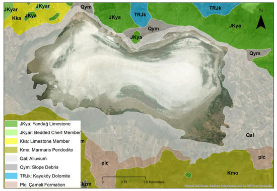
Figure 1.
Geological map of Akgöl Lake, Burdur.
The primary objective of this study is to map the spatial distribution of hydromagnesite deposits within the Akgöl (also known as Çorak Göl) basin—a dry lake located in the Lakes District of southwestern Türkiye—and to characterize the associated geochemical properties. Beyond documenting mineralization within the Akgöl basin itself, the research also aims to establish a methodological framework that can serve as a reference for identifying potential mineral distributions in other basins exhibiting similar geological characteristics. Accordingly, the study contributes to both regional-scale mineral exploration and geo-environmental assessment efforts, while also demonstrating the applicability of remote sensing and geostatistical modeling techniques in mineral prospecting workflows.
2. Materials and Methods
2.1. Field and Laboratory Studies
In order to determine the spatial distribution of some minerals (Hydromagnesite, Biotite, Dolomite, and Chamosite) within the Akgöl (Çorak Göl) lake basin, located within the provincial boundaries of Burdur and Denizli in Türkiye, a total of 70 samples were collected along three north–south-oriented profiles in 2022 (Figure 2a,b). These samples, taken from 70 distinct locations, consist of sand–clay mixed material from the dry lakebed. The collected samples were analyzed using X-Ray Fluorescence (XRF) (Brand: SPECTRO XEPOS, SPECTRO Analytical Instruments GmbH, Kleve, Germany), X-Ray Diffraction (XRD) (semi-quantitatively) (Brand: GNR, Agrate Conturbia, Italy), and spectroradiometry (Brand: ASD Field Spec Pro4, ASD Inc., Boulder, CO, USA). XRF and XRD data for each sample are presented in the Supplementary Excel File S1.
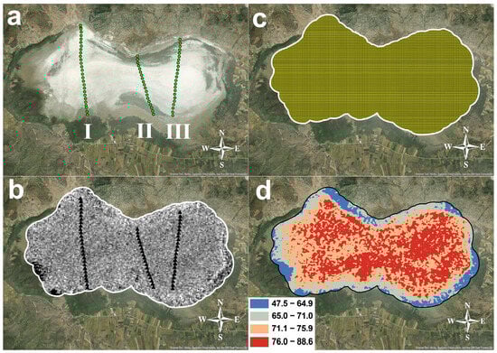
Figure 2.
Akgöl Lake. (a) Sampling points: I—First profile, II—Second profile, and III—Third profile; (b) Pre-processed ASTER satellite image; (c) geospatial point set on Akgöl Lake image; (d) Hydromagnesite distribution map.
2.1.1. Sample Collection
During the fieldwork, three sampling profiles were established to model the entire lake surface (Figure 2a). Starting from the left, samples were collected from 28 locations along the first profile (Nos. 1–28), 19 locations along the second profile (Nos. 29–47), and 23 locations along the third profile (Nos. 48–70), resulting in a total of 70 sampling locations. For each sample, the GPS coordinates were recorded (Garmin GPSMAP 65s; WGS84 reference system), and the sample was photographed together with its corresponding sample bag (Canon EOS 600D: Canon Inc., Tokyo, Japan) (Figure 2a,b).
2.1.2. Laboratory Analysis Procedures
The sediment samples collected from Akgöl were subjected to a series of preparatory and analytical procedures to ensure their suitability for mineralogical and geochemical characterization. Initially, all samples were processed using a crusher–grinder machine (JA-054 Halkalı Grinder: Jeotest, Ankara, Türkiye) located at the Earthquake and Structural Technologies Research Laboratory of Pamukkale University. Each sample was ground for a duration of 24 s to obtain a fine, homogeneous powder suitable for laboratory analysis. This standard grinding time was selected to ensure consistency across all samples while minimizing heat-induced alteration of mineral structures. Following the grinding process, the prepared powders were systematically analyzed using three analytical techniques: X-Ray Fluorescence (XRF) (Detector Type: Palladium Detector (Pd); Cooling System: Peltier Cooling; Gas Type: Helium (He) (Flow rate during measurement: 80–85 L/h); Measurement Range: Sodium–Uranium (Na–U)), X-Ray Diffraction (XRD) (semi-quantitatively) (X-Ray Source: Cu-Kα with Ni filter; Source Voltage: 40 kV; Source Current: 30 mA; Standard Scan Rate: 0.04° (2θ); Scan Range: 3° < 2θ < 90°), and spectroradiometry (measured range 350–2500 nm).
2.2. Data Processing
In parallel with the fieldwork, the phases involving remote sensing and GIS-based database development were carried out. Laboratory results obtained from XRD, XRF, and spectroradiometric analyses were digitized to create an attribute-rich dataset of the collected samples, which was then structured for use in mineral mapping. Following the identification of hydromagnesite content in the samples, the sampling points were georeferenced and overlaid onto a pre-processed ASTER satellite image. A total of 13,293 pixels covering the Akgöl basin were extracted from the ASTER imagery, and reflectance values at the center of each pixel were recorded to generate a geospatial point dataset. Subsequently, the hydromagnesite content (%) of these 13,293 points was estimated using a combination of measured hydromagnesite values (%) from 70 ground samples (provided in Supplementary Materials), the associated spectral band reflectance values, and a multiple regression model developed for predictive mapping. The mineral mapping process was performed using the Kriging interpolation method within the ArcGIS 10.3 software.
2.2.1. Digitization and Analysis of Sample Data
The data obtained from laboratory analyses were digitized and thoroughly examined using specialized software tools. The results of the X-Ray Diffraction (XRD) analyses were visualized through the Match! 3.4.2 software to identify mineral phases and assess the crystallographic characteristics of the samples. During this process, diffractograms of each sample were compared with standard XRD patterns from the internationally recognized RRUFF mineral database (Figure 3a–d).
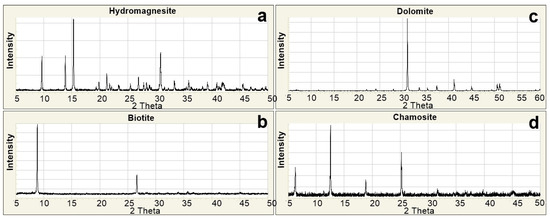
Figure 3.
Standard XRD patterns [48]. (a) Hydromagnesite; (b) Biotite; (c) Dolomite; (d) Chamosite.
These comparisons enabled both qualitative and quantitative determination of the mineral constituents. Based on the graphical evaluations, the mineral percentage distributions for all 70 samples were calculated and interpreted. The results of the spectroradiometric analyses were processed using ViewSpecPro 6.2.0 software to allow detailed examination of spectral reflectance characteristics (Figure 4a,b). The reflectance spectra for each sample were graphically visualized, with particular attention given to wavelengths critical for mineral differentiation. These spectral graphs facilitated the identification of characteristic spectral signatures of minerals and enabled cross-sample comparisons. Consequently, the integration of XRD and spectroradiometric data provided a comprehensive dataset for understanding the mineralogical and spectral properties of the samples.
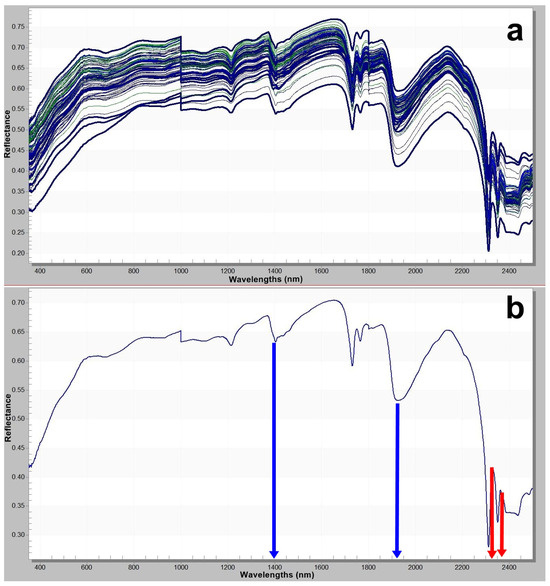
Figure 4.
(a) Spectral signatures of all samples; (b) representative spectral signature sample 25th (The blue arrow indicates hydroxyl groups and structural water at 1400 and 1900 nm, while the red arrow indicates carbonate groups in the 2300–2350 nm range.).
2.2.2. Image Processing
Preprocessing: In this study, an ASTER satellite image was utilized. The image was obtained from the United States Geological Survey (USGS) database (accessed on 10 October 2022; https://www.usgs.gov/). Since the downloaded ASTER image was in raw format, several preprocessing steps were performed using ENVI 5.3 software to prepare it for analysis. These steps included; (1) Radiometric calibration, (2) Atmospheric correction, and (3) Conversion to surface reflectance values.
Band Ratio Analysis: Following the preprocessing, specific bands from the Shortwave Infrared (SWIR) region of the ASTER image—namely bands 6, 7, and 8—were used for band ratio calculations. In order to enhance the detection of hydromagnesite on the image, a band ratio of (Band 6 + Band 8)/Band 7 was applied to generate high reflectance values [49] (Figure 2b). Subsequently, the pixel values corresponding to the geographic locations of field sample points (for which XRD-derived mineral percentages were available) were extracted and recorded on the satellite image (Figure 2c).
2.2.3. Database and Mineral Mapping
Following the tabulation of results obtained from XRF and XRD analyses (in Supplementary Materials), a geodatabase with the gdb extension was created using ArcGIS 10.3 software to serve as the foundation for spatial analysis and mapping. This geodatabase was populated with the central coordinates of each pixel within the Akgöl study area, along with their corresponding spectral reflectance values derived from the processed satellite imagery. To enable spatial interpolation, the raster-format satellite data were converted into vector point data, representing the center of each pixel as a distinct spatial unit. These point data were then prepared for surface modeling using the Kriging interpolation method. Through this approach, the limited number of ground sample points could be extrapolated to generate continuous mineral distribution maps across the entire lake surface. The Kriging method thus played a crucial role in translating discrete sample data into comprehensive and spatially continuous mineralogical maps (Figure 2d).
3. Results and Discussion
A comprehensive analysis of the XRD diffractograms and XRF results revealed the presence of various mineral phases within the samples. These analyses identified the occurrence of Hydromagnesite [Mg5(CO3)4(OH)2·(H2O)], Biotite [K(Mg,Fe2+)3(Al,Fe3+)Si3O10(OH,F)2], Dolomite [CaMg(CO3)2], and Chamosite [(Mg1.5Fe7.9Al2.6)(Si6.2Al1.8O20)(OH)16] in varying proportions across the samples. The relative abundances of these mineral phases differ from one sample to another, reflecting the mineralogical heterogeneity within the lake and underscoring the influence of micro-environmental variations on mineral formation. Notably, hydromagnesite was found to be the most dominant mineral phase, in terms of percentage content, in every sample analyzed. This finding strongly suggests that Akgöl represents a sedimentary environment particularly rich in hydromagnesite, and that this mineral plays a significant role in defining the overall geochemical character of the lake.
In Figure 2, the dark blue areas, representing hydromagnesite contents in the range of 47.5% to 64.9%, are predominantly located along the lake’s marginal zones. Adjacent to these, light grey regions indicate concentrations between 65% and 71%, forming an intermediate transitional belt. Further inward, orange-colored zones reflect values ranging from 71.1% to 75.9%. The highest concentrations, ranging from 76% to 88.6%, are shown in red and are primarily concentrated near the lake’s central zones. This distribution pattern clearly reveals an increasing gradient of mineral abundance toward the center of the lake.
Hydromagnesite is spectroradiometrically identified by the characteristic absorption of carbonate (CO32−) groups at the 2300 nm band. The 2500 nm band reflects the combined influence of both carbonate structures and molecular water bound within the mineral’s crystal lattice. This absorption is particularly prominent in hydrated minerals such as hydromagnesite. Additionally, the 1410 nm and 1910 nm wavelengths correspond to vibrational features of crystallized water (H2O) within the mineral. These bands provide insights into the hydration state of the mineral and typically manifest as deep absorptions in water-rich phases. These spectral characteristics are derived from the analysis of reflectance data obtained using portable spectroradiometers and enable highly accurate mineral identification.
Hydromagnesite contains four molecules of crystallized water (4H2O) and two hydroxyl (OH−) groups in its structure. The absorption bands observed around 1400 nm and 1900 nm arise from the combined vibrational effects of these H2O and OH groups [50,51,52]. The presence of hydromagnesite [Mg5(CO3)4(OH)2·4H2O] can be reliably identified through spectroradiometric analyses in the shortwave infrared (SWIR) region of the electromagnetic spectrum, particularly within the 2300–2500 nanometer (nm) range. These absorption features correspond to the vibrational modes of carbonate (CO32−) and hydroxyl (OH−) groups in the mineral structure and manifest as distinct decreases in spectral reflectance [52]. The absorption characteristics observed between 2300–2350 nm, attributed to carbonate groups and hydroxyl-related features, provide strong spectral evidence for the presence of hydromagnesite [52].
Although dolomite has also been detected in certain samples, the distinctive doublet absorption features at 2315 nm and 2340 nm are specific to hydromagnesite and serve as key spectral indicators differentiating it from other carbonate minerals. Upon examination of the spectral reflectance curves, the pronounced absorption bands at 1400 nm and 1900 nm—indicated by the blue arrow—are directly associated with the presence of hydroxyl groups and structural water within the mineral (Figure 4b). Meanwhile, the interval between 2300–2350 nm—indicated by the red arrow—reflects absorption by carbonate groups (Figure 4b). The concurrent presence of both absorption features confirms the dual nature of hydromagnesite as a hydrated carbonate mineral. These spectral characteristics serve as crucial diagnostic criteria for the identification and classification of this mineral in reflectance spectroscopy.
Numerous studies conducted on Lake Salda have demonstrated that the formation of hydromagnesite in this region is the result of microbial interactions, geochemical conditions, and unique lithological frameworks. For instance, Edwards et al. [53] highlighted the resemblance between hydromagnesite deposits in Lake Salda and the ‘White Rock’ formations on Mars, suggesting their potential relevance to habitability and microbial life signatures. Similarly, Demirel et al. [54] revealed that high ion concentrations combined with microbial organic polymers in Lake Salda, Acıgöl, and Lake Yarışlı trigger carbonate precipitation, thereby facilitating hydromagnesite formation. These findings are further supported by the saturation index-based analyses of Sezer [55] and the work of Sert et al. [56], which identified the presence of hydromagnesite in the Salda region. This mineral occurrence is considered rare at the global scale due to its specific lithological context, namely its formation within carbonate-rich lacustrine sediments under highly alkaline conditions, combined with the presence of magnesium in the surrounding rocks.
In this context, the high hydromagnesite content identified in the present study of the Akgöl Basin suggests that similar geochemical processes may be active in this environment. The observed similarities between the depositional settings of Akgöl and those of Lake Salda indicate that hydromagnesite formation is not confined to previously known localities. Instead, it may occur in other basins with comparable geological (e.g., source rock composition) and climatic (e.g., evaporation-driven) conditions, such as Lake Salda, Acıgöl, and Lake Yarışlı. These observations position Akgöl not only as a site of regional geological interest but also as a comparative model basin for future investigations into hydromagnesite-bearing environments.
4. Conclusions
Within the scope of this study, hydromagnesite values were estimated for a total of 13,293 pixels through multiple linear regression analysis, utilizing a custom-developed database. This approach enabled a quantitative assessment of the spatial distribution of hydromagnesite both within the interior and along the periphery of Akgöl. The resulting values were interpreted on a per-pixel basis, allowing for a detailed mapping of the mineral’s density and distribution across the lake and its surroundings. Consequently, a unique hydromagnesite distribution map for the study area was produced, serving as a valuable output for improving the understanding of the region’s geochemical characteristics.
The observed distribution pattern (Figure 2) is likely closely linked to the endorheic nature of Akgöl and the prevailing arid climatic conditions. One of the primary factors governing this pattern is the evaporation-driven precipitation mechanism. In closed-basin saline lakes such as Akgöl, evaporation tends to be more intense in the central parts of the basin. This process accelerates the saturation of the lake water in these areas, promoting increased mineral precipitation [24]. As a mineral that precipitates predominantly under alkaline conditions and in magnesium (Mg)-rich environments, hydromagnesite tends to accumulate at higher concentrations in the central zones—where such conditions prevail—corresponding to the red-colored regions on the distribution map.
Sedimentation processes also represent a significant factor influencing this spatial distribution. In the marginal areas of the lake—particularly those represented by blue and grey tones—it is likely that younger, fine-grained, and organic-rich sediments are more prevalent. These zones, which receive greater input from external materials, may exhibit lower magnesium (Mg) content compared to the lake’s center. In contrast, the central part of the lake, having experienced prolonged and stable sedimentation processes, has likely accumulated thicker, more mineralogically pure layers, which explains the elevated hydromagnesite concentrations observed in these areas.
Additionally, groundwater dynamics may play a role in this distribution pattern. If groundwater entering from beneath or along the margins of the lake is enriched in Mg, it could gradually contribute to increased mineral precipitation in the lake’s central zone. During the summer months, enhanced evaporation further promotes the accumulation and subsequent precipitation of magnesium sourced from groundwater, contributing to the formation of high-concentration mineral deposits.
Finally, Akgöl’s endorheic nature—characterized by the absence of an outlet—facilitates the retention and internal cycling of dissolved minerals, promoting their accumulation in the central basin. This phenomenon is commonly observed in other closed-basin saline lakes with similar geological and climatic conditions, such as Acıgöl and Lake Burdur. Taken together, these factors provide a scientifically coherent explanation for the increasing concentration gradient of hydromagnesite toward the center of the lake.
Additional geochemical factors influencing the distribution of hydromagnesite must also be considered. In particular, elevated pH levels and high Mg/Ca ratios are known to create favorable conditions for hydromagnesite formation [25]. The relatively stable and elevated values of these parameters in the central part of the lake likely contribute to the enhanced precipitation of the mineral in this zone.
Supplementary Materials
The following supporting information can be downloaded at: https://www.mdpi.com/article/10.3390/app152111536/s1, Table S1: Supplementary File (Results of XRF and XRD).
Author Contributions
A.C.B. and H.K. contributed to the study conception and design. Material preparation, data collection and analysis were performed by A.C.B. The first draft of the manuscript was written by A.C.B. and H.K. commented on previous versions of the manuscript. All authors have read and agreed to the published version of the manuscript.
Funding
This research was funded by the Pamukkale University, Scientific Research Projects Coordinatorship grant number [2022FEBE034].
Institutional Review Board Statement
Not applicable.
Informed Consent Statement
Not applicable.
Data Availability Statement
The original contributions presented in this study are included in the article/Supplementary Materials. Further inquiries can be directed to the corresponding author(s).
Acknowledgments
I sincerely thank my dear wife, Eda Bayraktaroğlu, and my daughter, Çağla Bayraktaroğlu, for their valuable help and support during the field and laboratory work. I am also grateful to Musa Tataroğlu (Lecturer at Pamukkale University), my father, Şahin Şevki Bayraktaroğlu, and Ömer Bozkaya for their contributions to the study.
Conflicts of Interest
The authors declare no conflicts of interest.
References
- Xu, Y.; Cheng, Q. A Fractal Filtering Technique for Processing Regional Geochemical Maps for Mineral Exploration. Geochem. Explor. Environ. Anal. 2001, 1, 147–156. [Google Scholar] [CrossRef]
- Kreuzer, O.P.; Yousefi, M.; Nykänen, V. Introduction to the Special Issue on Spatial Modelling and Analysis of Ore-Forming Processes in Mineral Exploration Targeting. Ore Geol. Rev. 2020, 119, 103391. [Google Scholar] [CrossRef]
- Wang, J.; Zuo, R. An Extended Local Gap Statistic for Identifying Geochemical Anomalies. J. Geochem. Explor. 2016, 164, 86–93. [Google Scholar] [CrossRef]
- Wang, J.; Zuo, R.; Liu, Q. Mapping Geochemical Anomalies by Accounting for the Uncertainty Of-Related Elemental Associations. Solid Earth 2024, 15, 731–746. [Google Scholar] [CrossRef]
- Kirkwood, C.; Cave, M.; Beamish, D.; Grebby, S.; Ferreira, A. A Machine Learning Approach to Geochemical Mapping. J. Geochem. Explor. 2016, 167, 49–61. [Google Scholar] [CrossRef]
- Franks, D.M.; Keenan, J.; Hailu, D. Mineral Security Essential to Achieving the Sustainable Development Goals. Nat. Sustain. 2023, 6, 21–27. [Google Scholar] [CrossRef]
- Loubser, M.; Verryn, S. Combining XRF and XRD Analyses and Sample Preparation to Solve Mineralogical Problems. S. Afr. J. Geol. 2008, 111, 229–238. [Google Scholar] [CrossRef]
- Secchi, M.; Zanatta, M.; Borovin, E.; Bortolotti, M.; Kumar, A.; Giarola, M.; Sanson, A.; Orberger, B.; Daldosso, N.; Gialanella, S.; et al. Mineralogical Investigations Using XRD, XRF, and Raman Spectroscopy in a Combined Approach. J. Raman Spectrosc. 2018, 49, 1023–1030. [Google Scholar] [CrossRef]
- Bortolotti, M.; Lutterotti, L.; Pepponi, G. Combining XRD and XRF Analysis in One Rietveld-like Fitting. Powder Diffr. 2017, 32 (Suppl. S1), S225–S230. [Google Scholar] [CrossRef]
- Howarth, R.J. A History of Regression and Related Model-Fitting in the Earth Sciences (1636?–2000). Nat. Resour. Res. 2001, 10, 241–286. [Google Scholar] [CrossRef]
- Coburn, T.C.; Freeman, P.A.; Attanasi, E.D. Empirical Methods for Detecting Regional Trends and Other Spatial Expressions in Antrim Shale Gas Productivity, with Implications for Improving Resource Projections Using Local Nonparametric Estimation Techniques. Nat. Resour. Res. 2012, 21, 1–21. [Google Scholar] [CrossRef]
- Granian, H.; Tabatabaei, S.H.; Asadi, H.H.; Carranza, E.J.M. Multivariate Regression Analysis of Lithogeochemical Data to Model Subsurface Mineralization: A Case Study from the Sari Gunay Epithermal Gold Deposit, NW Iran. J. Geochem. Explor. 2015, 148, 249–258. [Google Scholar] [CrossRef]
- Kumar, N.; Sinha, N.K. Geostatistics: Principles and Applications in Spatial Mapping of Soil Properties. In Geospatial Technologies in Land Resources Mapping, Monitoring and Management; Reddy, G.P.O., Singh, S.K., Eds.; Springer International Publishing: Cham, Switzerland, 2018; pp. 143–159. [Google Scholar] [CrossRef]
- Langkoke, R.; Ahmad, A.; Thamrin, M.; Husain, R.; Iqbal, M. Geocomputation and Spatial Analysis Applied for Geological Mapping: A Case Study in Palopo, South Sulawesi, Indonesia. J. Ecosolum 2024, 13, 68–81. [Google Scholar] [CrossRef]
- Hollingbery, L.A.; Hull, T.R. The Thermal Decomposition of Natural Mixtures of Huntite and Hydromagnesite. Thermochim. Acta 2012, 528, 45–52. [Google Scholar] [CrossRef]
- Hu, Q.F.; Song, L.Y.; Hu, X.X. Study on Exploitation and Utilization of Basic Magnesite. Inorg. Chem. Ind. 2005, 11, 44–46. [Google Scholar]
- Xi, Y. Study on Purification of a Low-Grade Hydromagnesite Ore in Tibet Area. Master’s Thesis, Liaoning University of Science and Technology, Anshan, China, 2020. [Google Scholar]
- Lin, Y.; Zheng, M.; Ye, C.; Power, I.M. Rare Earth Element and Strontium Isotope Geochemistry in Dujiali Lake, Central Qinghai-Tibet Plateau, China: Implications for the Origin of Hydromagnesite Deposits. Geochemistry 2019, 79, 337–346. [Google Scholar] [CrossRef]
- Li, X.H. Genesis and Prospecting Criteria of Naqu Shui Magnesite Deposit in Tibet. China Well Rock Salt 2022, 53, 21–24. [Google Scholar]
- van der Meer, F.D.; van der Werff, H.M.A.; van Ruitenbeek, F.J.A.; Hecker, C.A.; Bakker, W.H.; Noomen, M.F.; van der Meijde, M.; Carranza, E.J.M.; de Smeth, J.B.; Woldai, T. Multi- and Hyperspectral Geologic Remote Sensing: A Review. Int. J. Appl. Earth Obs. Geoinf. 2012, 14, 112–128. [Google Scholar] [CrossRef]
- Jiao, L.-L.; Zhao, P.-C.; Liu, Z.-Q.; Wu, Q.-S.; Yan, D.-Q.; Li, Y.-L.; Chen, Y.-N.; Li, J.-S. Preparation of Magnesium Hydroxide Flame Retardant from Hydromagnesite and Enhance the Flame Retardant Performance of EVA. Polymers 2022, 14, 1567. [Google Scholar] [CrossRef]
- Young, G.A. Hydromagnesite Deposits of Atlin, B.C. In Geological Survey of Canada Summary Report; Geological Survey of Canada: Ottawa, ON, Canada, 1916; pp. 50–61. [Google Scholar]
- Zhao, T.; Dai, J.; Zhao, Y.; Ye, C. MTMF Method for Hydromagnesite Determination Based on Landsat8 and ZY1-02D Data: A Case Study of the Jiezechaka Salt Lake in Tibet. Aquat. Geochem. 2024, 30, 219–238. [Google Scholar] [CrossRef]
- Renaut, R.W. Morphology, Distribution, and Preservation Potential of Microbial Mats in the Hydromagnesite-Magnesite Playas of the Cariboo Plateau, British Columbia, Canada. Hydrobiologia 1993, 267, 75–98. [Google Scholar] [CrossRef]
- Braithwaite, C.J.R.; Zedef, V. Hydromagnesite Stromatolites and Sediments in an Alkaline Lake, Salda Golu, Turkey. J. Sediment. Res. 1996, 66, 991–1002. [Google Scholar] [CrossRef]
- Hatjilazaridou, K.; Chalkiopoulou, F.; Grossou-Valta, M. Greek Industrial Minerals: Current Status and Trends. Ind. Miner. 1998, 369, 45–63. [Google Scholar]
- Yılmaz Atay, H.; Çelik, E. Use of Turkish Huntite/Hydromagnesite Mineral in Plastic Materials as a Flame Retardant. Polym. Compos. 2010, 31, 1692–1700. [Google Scholar] [CrossRef]
- Liodakis, S.; Tsoukala, M. Environmental Benefits of Using Magnesium Carbonate Minerals as New Wildfire Retardants Instead of Commercially Available, Phosphate-Based Compounds. Environ. Geochem. Health 2010, 32, 391–399. [Google Scholar] [CrossRef]
- Zheng, M.P.; Xiang, J.; Wei, X.J.; Zheng, Y. Salt Lake on the Tibetan Plateau; Beijing Science & Technology Press: Beijing, China, 1989. [Google Scholar]
- Jiang, T.M.; Ji, L.M.; Cheng, H.D.; Li, B.K.; Li, G.; Ma, H.Z.; Zhang, X.Y.; Li, C.Z.; Ma, X.H.; Zhang, P.C. Algae Mineralization Experiment and Genetic Analysis of Hydromagnesite in Bangor Lake, Xizang (Tibet). Geol. Rev. 2021, 67, 1709–1726. [Google Scholar]
- Zhao, Y. Principles and Methods for Remote Sensing Application and Analysis; Science Press: Beijing, China, 2003; pp. 415–416. [Google Scholar]
- Yang, J.Z.; Zhao, Y.L. Technical Features of Remote Sensing and Its Application in the Geological Survey and Mineral Resources Survey. Miner. Explor. 2015, 6, 529–534. [Google Scholar]
- Dai, J.J.; Wang, D.H.; Wang, H.Y. A review of remote sensing survey of rare earth mineral resources in China. Acta Geol. Sin. 2019, 93, 1270–1278. [Google Scholar]
- Geng, X.X.; Yang, J.M.; Zhang, Y.J.; Yao, F.J. Application of RS Technology to Geology and Ore Deposit Research and the Development Prospect. Contrib. Geol. Miner. Resour. Res. 2008, 2, 89–93. [Google Scholar]
- Russell, M.J.; Ingham, J.K.; Zedef, V.; Maktav, D.; Sunar, F.; Hall, A.J.; Fallick, A.E. Search for Signs of Ancient Life on Mars: Expectations from Hydromagnesite Microbialites, Salda Lake, Turkey. J. Geol. Soc. Lond. 1999, 156, 869–888. [Google Scholar] [CrossRef]
- Salaj, S.S.; Upadhyay, R.; Srivastav, S.K. Mineral Abundance Mapping Using Hyperion Dataset in Part of Udaipur Dist Rajasthan, India. In Proceedings of the 14th Annual International Conference and Exhibition on Geospatial Information Technology and Applications, Gurgaon, India, 7–9 February 2012. [Google Scholar]
- Pour, A.B.; Hashim, M. Alteration Mineral Mapping Using ETM+ and Hyperion Remote Sensing Data at Bau Gold Field, Sarawak, Malaysia. IOP Conf. Ser. Earth Environ. Sci. 2014, 18, 012149. [Google Scholar] [CrossRef]
- Mohammady Oskouei, M.; Babakan, S. Role of Smile Correction in Mineral Detection on Hyperion Data. J. Min. Environ. 2016, 7, 261–272. [Google Scholar] [CrossRef]
- Kargi, H. Principal Components Analysis for Borate Mapping. Int. J. Remote Sens. 2007, 28, 1805–1817. [Google Scholar] [CrossRef]
- Kavak, K.S. Recognition of Gypsum Geohorizons in the Sivas Basin (Turkey) Using ASTER and Landsat ETM+ Images. Int. J. Remote Sens. 2005, 26, 4583–4596. [Google Scholar] [CrossRef]
- Öztan, N.S. Evaporate Mapping in Bala Region (Ankara) by Remote Sensing Techniques. Master’s Thesis, Middle East Technical University, Ankara, Turkey, 2008. [Google Scholar]
- Öztan, N.S.; Süzen, M.L. Mapping Evaporate Minerals by ASTER. Int. J. Remote Sens. 2011, 32, 1651–1673. [Google Scholar] [CrossRef]
- Caceres, F.; Ali-Ammar, H.; Pirard, E. Mapping Evaporitic Minerals in Sud Lipez Salt Lakes, Bolivia, Using Remote Sensing. In Remote Sensing and Spectral Geology; Society of Economic Geologists: Littleton, CO, USA, 2009; pp. 199–208. [Google Scholar] [CrossRef]
- Özyavaş, A. Assessment of Image Processing Techniques and ASTER SWIR Data for the Delineation of Evaporates and Carbonate Outcrops along the Salt Lake Fault, Turkey. Int. J. Remote Sens. 2016, 37, 770–781. [Google Scholar] [CrossRef]
- Bölükbaşı, A.S. Elmalı (Antalya)–Açıgöl–Burdur Gölü (Burdur) Korkuteli (Antalya) Arasında Kalan Elmalı Napları Jeolojisi. In TPAO Raporları; No: 2415; TPAO: Ankara, Turkey, 1987. [Google Scholar]
- Bilgin, Z.R.; Karaman, T.; Öztürk, Z.; Şen, M.A.; Demirci, A.R. Yeşilova-Akgöl Civarının Jeolojisi; No: 9071; Jeoloji Etütleri Dairesi Başkanlığı: Ankara, Turkey, 1990. [Google Scholar]
- Yılmaz, Y.; Berberoğlu, E.; Gülle, İ. Burdur’un Doğası; Pegasus Görsel İletişim: Çorum, Turkey, 2019. [Google Scholar]
- Lafuente, B.; Downs, R.T.; Yang, H.; Stone, N. The Power of Databases: The RRUFF Project. In Highlights in Mineralogical Crystallography; Armbruster, T., Danisi, R.M., Eds.; W. De Gruyter: Berlin, Germany, 2015; pp. 1–30. [Google Scholar]
- Son, Y.-S.; Lee, G.; Lee, B.H.; Kim, N.; Koh, S.-M.; Kim, K.-E.; Cho, S.-J. Application of ASTER Data for Differentiating Carbonate Minerals and Evaluating MgO Content of Magnesite in the Jiao-Liao-Ji Belt, North China Craton. Remote Sens. 2022, 14, 181. [Google Scholar] [CrossRef]
- Hunt, G.R. Spectral Signatures of Particulate Minerals in the Visible and near Infrared. Geophysics 1977, 42, 501–513. [Google Scholar] [CrossRef]
- Gaffey, S.J. Spectral Reflectance of Carbonate Minerals in the Visible and near Infrared (0.35–2.55 Microns); Calcite, Aragonite, and Dolomite. Am. Mineral. 1986, 71, 151–162. [Google Scholar]
- Clark, R.N. Spectroscopy of Rocks and Minerals and Principles of Spectroscopy. In Manual of Remote Sensing, Volume 3, Remote Sensing for the Earth Sciences; Rencz, A.N., Ed.; Wiley: Hoboken, NJ, USA, 1999; pp. 3–58. [Google Scholar]
- Edwards, H.G.M.; Moody, C.D.; Newton, E.M.; Villar, S.E.J.; Russell, M.J. Raman Spectroscopic Analysis of Cyanobacterial Colonization of Hydromagnesite, a Putative Martian Extremophile. Icarus 2005, 175, 372–381. [Google Scholar] [CrossRef]
- Demirel, C.; Balcı, N.; Akçer-Ön, S. Investigation of Biogeochemical Processes Affecting Modern Carbonate Precipitation in Lake Acıgöl, Lake Yarışlı And Lake Salda. In Proceedings of the Türkiye Kuvaterner Sempozyumu (TURQUA), İstanbul, Turkey, 8–11 May 2016. [Google Scholar]
- Sezer, B. Salda Gölü Güncel Magnezyum Çökellerinin Kristalizasyon Mekanizması ve SI (Saturation Index) Özellikleri. Master’s Thesis, İstanbul Teknik Üniversitesi, İstanbul, Turkey, 2004. [Google Scholar]
- Sert, M.; Arsoy, Z.; Çelik, M.Y. Salda Gölünün Kıyı Şeridini Oluşturan Kayaçların Karakterizasyonu. Curr. Acad. Stud. 2018, 1, 655–668. [Google Scholar]


Disclaimer/Publisher’s Note: The statements, opinions and data contained in all publications are solely those of the individual author(s) and contributor(s) and not of MDPI and/or the editor(s). MDPI and/or the editor(s) disclaim responsibility for any injury to people or property resulting from any ideas, methods, instructions or products referred to in the content. |
© 2025 by the authors. Licensee MDPI, Basel, Switzerland. This article is an open access article distributed under the terms and conditions of the Creative Commons Attribution (CC BY) license (https://creativecommons.org/licenses/by/4.0/).