Abstract
The generalisation of Deep Learning (DL) models under extrapolated usage conditions, particularly in the context of fault diagnosis, remains a significant challenge. Traditional methods encounter difficulties in terms of adaptability, necessitating extensive retraining when confronted with evolving conditions and unanticipated fault patterns. Moreover, existing DL approaches often demonstrate a lack of robustness in dynamic environments due to their limited capacity for generalisation. To address these limitations, this work introduces a novel Curriculum Learning (CL)-based approach, the Residual Singular Value Decomposition Curriculum Learning algorithm (ReSVD-CL), which integrates a Long Short-Term Memory (LSTM) model to capture temporal dependencies in fault patterns and Singular Value Decomposition (SVD) preprocessing to enhance feature representation. A complexity-based criterion segments the dataset into subsets, which are gradually incorporated into training via a pacing function. A comparison of ReSVD-CL with existing methods, such as Baby-Step Curriculum Learning (BS-CL), One-Pass Curriculum Learning (OP-CL) and baseline approaches of fault diagnosis, demonstrates that ReSVD-CL attains superior classification performance, particularly in extrapolated scenarios. The approach facilitates continuous adaptation to new usage profiles without the necessity of full retraining, thereby reducing computational costs and accelerating convergence. The study maintains a strong diagnostic performance with minimal usage profiles, thus demonstrating the potential of combining CL with dimension reduction and temporal modelling to develop more efficient and adaptable fault diagnosis systems.
1. Introduction
In the modern industrial context, characterised by accelerated advancements, industrial equipment has evolved to become increasingly intricate, adaptable, and automated. Within the domain of industrial big data, Intelligent Fault Diagnosis (IFD) has emerged as a pivotal element of Pronostic and Health Management (PHM) [1,2]. IFD methodologies are predicated on the identification of fault categories through the exploitation of relationships between monitoring signals and fault patterns [3]. Deep Learning (DL)-based approaches relied on autonomous feature extraction but assume independent and identically distributed data [4]. More recently, Transfer Learning (TL) has addressed domain shifts and improved adaptability under different conditions [5]. However, ensuring generalisation across different working conditions remains a challenge [6]. This is of particular pertinence in the context of electric motors, where the presence of complex fault patterns and variable operational conditions necessitates the employment of advanced diagnostic methodologies. These methodologies will be the focus of the ensuing sections.
This study builds upon established physical modelling and hybrid cooperative approaches to fault diagnosis, which combine theoretical system knowledge with data-driven methods [7,8]. While physical models provide interpretability and precise detection when well-defined, they face challenges related to model complexity and prediction uncertainty [9]. Data-driven models, although requiring large datasets, often lack transparency and interpretability [10]. Hybrid models leverage the advantages of both, enhancing accuracy and generalisation in fault diagnosis [7]. The present work advances these approaches by proposing a novel hybrid framework designed to improve fault diagnosis performance under extrapolated operating conditions, thus addressing current limitations in the field. Curriculum Learning (CL) has recently been explored in IFD to enhance model robustness in challenging scenarios such as few-shot learning or noisy, heterogeneous data environments. For instance, CL strategies have been integrated into federated learning frameworks to mitigate the impact of label noise [11,12] or combined with meta-learning for improved fault diagnosis with limited annotated samples [13]. A variant of this approach also introduces a spectral norm-based curriculum metric to guide model training across few-shot tasks [14]. While these approaches demonstrate promising results, they remain constrained by context-specific assumptions—such as uniform noise distributions or fixed task complexity—and often lack integration with physical signal properties. In response to these limitations, the present study introduces a new Curriculum Learning (CL)-based approach, the Residual Singular Value Decomposition Curriculum Learning algorithm (ReSVD-CL), which integrates a Long Short-Term Memory (LSTM) model to capture temporal dependencies in fault patterns and Singular Value Decomposition (SVD) preprocessing to enhance feature representation. The expected benefits is generalisability as this framework incrementally incorporates complex operating conditions while preserving previously acquired knowledge.Therefore, the approach addresses both extrapolation and computational efficiency, and demonstrates improved generalisation compared to baseline and state-of-the-art methods in vibration-based diagnosis of electric motors.
1.1. Fault Diagnosis of Electric Motors
The performance of electric motors is susceptible to compromise from both mechanical (e.g., bearing failures, misalignments) and electrical faults (e.g., overloads, insulation breakdowns) [15,16,17]. Bearing issues are a significant contributing factor to motor failure, thus prompting interest in [18].
Various methods are used to detect bearing faults, including acoustic emission, temperature monitoring, motor current analysis, wear debris analysis, and vibration analysis. Acoustic emission detects structural changes due to cracking but is sensitive to external noise, leading to false alarms [19,20,21]. Temperature monitoring detects heating failures but may miss early-stage faults. Motor current analysis provides a non-intrusive approach but lacks precision in fault location [22]. Wear debris analysis is effective for severe faults but fails to detect early damage [23].
Vibration analysis, including time-domain, frequency-domain, and time-frequency-domain techniques, is widely used [24,25,26]. Time-domain methods offer rapid fault detection but lack frequency distribution details, while frequency-domain techniques provide deeper insights but require expert interpretation. Time-frequency methods, like wavelet transform, are better for non-stationary signals but demand high computational resources [27,28,29]. Additionally, Artificial Neural Networks (ANNs) and Fast Fourier Transform (FFT) are particularly used in the context of large datasets [30,31] but require extensive data for ANNs and struggle with non-stationary signals for FFT [32,33,34].
Future developments in fault diagnosis are likely to include a broader array of diagnostic techniques. Vibration analysis and motor current analysis could be be enhanced with Deep Learning (DL) algorithms, enabling these technologies to learn from historical data and adapt to new patterns of motor behaviour [35,36].
This will allow for more comprehensive monitoring of electric motor systems, encompassing not just mechanical issues but also electrical and thermal anomalies. Despite the advances made in the field, the development of a generalised, practical approach for accurate and explainable diagnosis of various motor faults remains an ongoing challenge [37,38] in different usage conditions.
1.2. Generalisation to Extrapolated Operating Conditions
Many industrial processes, due to their intrinsic complexity arising from non-linear relationships and numerous involved variables, require constant optimization. The relationships between inputs and outputs of these complex systems can be modeled using industrial data, fundamental principles, or a combination of both, known as hybrid modeling. Hybrid modeling, which leverages the advantages of both data-driven and physics-based models, offers a balance between process accuracy and data quality. Fundamental principles and, more generally, physics-based models provide precise analytical tracking of phenomena occurring in the system, while real data, readily collected from the system, qualitatively and quantitatively capture the system’s real-time behavior. Several in-depth studies [39,40,41] have reinforced the choice to proceed with this type of modeling to solve this problem. For instance, Guo et al. [42] proposed a Physics-Guided Neural Network (PGNN) to model chiller performance in HVAC (Heating, Ventilation, and Air Conditioning) systems, where physical constraints are embedded within the neural network structure to enhance extrapolation capabilities beyond the original training data range. Similarly, in the context of electromagnetic wave propagation, Huang et al. [43] developed a physics-guided machine learning model that incorporates deterministic knowledge and demonstrates strong extrapolation capabilities across unseen terrains. In their seminal work, Gallup et al. [44] demonstrated that the incorporation of scientific knowledge into neural networks, facilitated by hybrid architectures, physics-guided loss functions, and physics-based initialisation, enhances the efficiency and precision of training processes. Li et al. [45] developed a physics-embedded graph neural network that integrates heat diffusion principles to reconstruct temperature fields from sparse sensors. This approach significantly improves accuracy and robustness in out-of-distribution scenarios by embedding physical laws directly into the network architecture. Finally, Elhamod et al. [46] identify the challenge posed by competing physics-guided losses with conflicting gradients. They propose an adaptive weighting strategy during training to achieve more generalisable solutions in complex scientific problems, such as quantum mechanics and electromagnetic propagation.
1.3. Contributions
This study addresses the issue of fault diagnosis in extrapolated usage conditions, with a particular focus on enhancing model robustness. These conditions refer to operational scenarios that differ significantly from those originally considered during the motor’s design or initial deployment. Examples include the reuse of electric motors in new industrial contexts, or usage involving atypical stress patterns such as frequent restarts, unexpected collisions, or load variations. It is acknowledged that a system may encounter new usage scenarios following model development, and the proposed method aims to address this by reusing the initial implementation, tailored to the input data of the physical model. Following the numerical validation of the model on a classification problem [47], the focus shifts to the analysis of the characteristics of the input data. Enhancing model robustness involves expanding input databases [48]. However, large datasets can hinder the model’s ability to detect and generalise correlations between variables, making it difficult to distinguish profiles that could lead to different response values. To address this, the approach proposes progressively integrating increasingly complex training data during model training. Curriculum learning (CL), as pioneered by Selfridge et al. in 1985 and grounded in human learning processes [49], has been a subject of extensive research. This approach entails the presentation of progressively challenging data subsets to promote machine learning. Subsequent research by Elman in 1993 [50] demonstrated that recurrent neural networks exhibit optimal performance in grammar learning when data difficulty escalates over time. Subsequently, Bengio et al. formalised CL in machine learning, as cited in Bengio et al. [51]. The aim of this paper is to demonstrate that incrementally adding data or knowledge improves the predictive model performance compared to traditional full learning. This approach allows the system to adapt to new usage profiles without overwriting previously trained network weights, ensuring model stability. In a related development, Wang et al. have proposed a novel architecture that integrates CL to address domain and category shifts in fault diagnosis, thereby demonstrating its potential for online fault diagnosis [52].
The methodology is developed around the input data of a specific use case, although it is designed to be generalizable to other industrial systems. The primary objective of this study is to improve the robustness and adaptability of fault diagnosis models when exposed to previously unseen operating conditions, a common challenge in industrial systems. To this end, a novel methodology is proposed, combining CL with singular value decomposition-based dimensionality reduction. The resulting framework, ReSVD-CLNet, incrementally integrates increasingly complex training data while preserving previously acquired knowledge, thereby enabling the model to adapt to new usage profiles without retraining from scratch. This hybrid approach promotes generalisation while managing computational cost and training stability. The main contributions of this paper are threefold. First, a novel CL strategy is proposed, adapted to the classification of multivariate time series faults, which progressively enriches the model as new data becomes available. This approach combines CL with dimension reduction to enable cost-effective training. Then, curriculum learning enhances the generalisation of the Long Short-Term Memory (LSTM) model to new usage profiles in the context of failure diagnosis. Third, comparative evaluation with existing strategies demonstrates the superior generalisation of this method when confronted with extrapolated operating conditions. The findings demonstrate that the proposed approach significantly enhances classification accuracy and generalisation performance in extrapolated scenarios, outperforming baseline and state-of-the-art methods. The structure of the paper is as follows: Section 2 reviews existing work on CL and its limited application to time series classification. Section 3 details the proposed methodology and the design of the ReSVD-CLNet framework. Section 4 presents the experimental setup and investigates the properties of the CL strategy, followed by a comparative evaluation in Section 5. The results and discussion are presented in Section 6, and the conclusions are drawn in Section 7.
2. Related Works
2.1. Concept of Curriculum Learning and Applications
Continuation methods are optimisation strategies that start by solving a simplified version of a problem to obtain a global perspective before gradually increasing complexity to refine the solution [53]. CL follows a similar principle by structuring the training process, beginning with simpler examples and progressively introducing more complex ones [54]. This approach has been shown to enhance performance and accelerate training, particularly in deep reinforcement learning and other deep learning applications [55]. By guiding models to acquire fundamental concepts before tackling difficult tasks, CL mitigates issues related to poor convergence and local minima [56].
Designing an effective curriculum remains a central challenge in curriculum learning (CL), with several studies proposing different approaches to ordering training samples based on their complexity [51,57,58,59]. For instance, Bengio et al. [51] define a curriculum as a sequence of training criteria over T training steps, where each criterion assigns different weights to training samples from the target dataset (see Figure 1). Formally, at step i, the curriculum is expressed as:
where represents the distribution of training samples, and (with ) defines their weighting at step i. The effectiveness of CL depends on how well these criteria are designed, which remains an open challenge (see Figure 1).
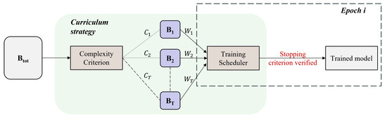
Figure 1.
Founding concept of curriculum learning illustrated for an epoch (derived from [51]). represents the initial basis of learning data and is the set of sub-bases determined by the complexity criterion.
Some literature reviews [59,60,61] emphasise that the choice of curriculum learning strategy should be tailored to the specific characteristics of the problem and data. A common principle is to begin training with simpler examples before progressing to more complex ones, a notion often referred to as learning from easy to hard. Most CL methods share two key components: a training scheduler and a complexity measure [59]. These elements form the foundation of the approach developed in this study. Depending on the nature of the input data, the complexity criterion is set to assess the relative ease of each example in the dataset. Observations are then sorted increasingly from least complex to most complex. They are subsequently fed into the scheduling function. The scheduling function defines the sampling to be applied at each epoch to slice the training dataset into subsets and insert the subset at the opportune moment. Although scheduling functions are empirically constructed to fit the specific constraints of the problem at hand, they can be categorized based on their typology (see below Section 2.2). Thus, curriculum learning is generally characterized as a learning technique that trains the predictive model using the curriculum principle (see Figure 1) introduced above. It has been employed for various tasks such as semi-supervised object detection on increasingly unlabeled images [62,63], machine translation on increasingly noisy data [64], or longer sentences [65], and image generation with GANs (Generative Adversarial Networks) using CL to propose the best combination of discriminators [66] or to estimate the impact of image difficulty on results [67].
The comprehensive and recent review by [59] demonstrates that the curriculum is primarily applied to Natural Language Processing and object detection tasks but is non-existent for failure classification tasks. Regarding the case study of time sequences, a similar rationale is found in the exploration of stock prices [68]. Despite its advantages, CL is rarely applied in time-series regression tasks due to the challenge of defining a complexity measure for sequential data [69]. Existing CL-based approaches often rely on predefined difficulty levels, static data partitioning, or heuristics that lack adaptability [60]. Moreover, many methods fail to ensure model stability when new usage conditions arise, leading to performance degradation over time [70].
The present work introduces a novel CL-based approach tailored to time-series regression tasks, particularly in industrial systems where predictive models must generalise to evolving usage conditions. In order to identify a suitable curriculum, it is essential to undertake a thorough analysis of the existing methods in place and their respective limitations.
2.2. Curriculum Learning Methods
According to [60], existing Curriculum Learning methods can be divided into predefined CL and automatic CL. The main difference between these two methods is that predefined CL requires domain expert knowledge, unlike automatic CL.
2.2.1. Predefined CL
Predefined CL, or Predefined Curriculum Learning, refers to a method in which the components of the curriculum, such as difficulty measurement and training scheduling, are manually designed by experts based on prior knowledge of the specific data and tasks. In other words, human experts define the sequence in which training examples are presented to the model, as well as how the difficulty of these examples is measured. This approach is based on a priori knowledge of the data and task characteristics, and it is often used when expert information is available to design a curriculum tailored to specific scenarios. Commonly employed complexity measures are based on data characteristics, including complexity, diversity, and noise estimation. These measures, primarily designed for image and text data, aim to assess task difficulty using criteria such as sentence length [64], the number of objects in images, or distributional diversity. Complexity reflects the structure of data examples, diversity evaluates the variety of data, while noise estimation measures the level of disturbance in examples [71]. These measures, often linked to complexity, influence the model’s capabilities and the training complexity involved. Predefined training schedulers encompass four common types: discrete schedulers, continuous schedulers, fixed schedulers, and adaptive schedulers. Discrete schedulers adjust the data subset at fixed intervals, while continuous schedulers modify it at each epoch. Fixed schedulers follow a predefined schedule regardless of model feedback, whereas adaptive schedulers adjust based on model performance. Despite the effectiveness of predefined CL, it lacks flexibility. The components of the predefined curriculum remain fixed throughout the training process, which can limit the model’s adaptability to changes in performance or learning needs.
2.2.2. Automatic CL
Automatic CL, or Automatic Curriculum Learning, is a method in which at least one of the curriculum components, such as the measurement of example complexity and training scheduling, is learned by models or data-based algorithms [72]. Unlike predefined CL where the curriculum components are manually defined by experts, the automatic approach allows the system to dynamically adapt the curriculum based on the model’s performance during training. This method aims to reduce reliance on human expertise [60] and enables the model to learn to select examples and adjust training difficulty autonomously. There are three main methodologies for automatic curriculum learning: self-paced learning [73,74], transfer from a pre-trained teacher model [75], using reinforcement learning models as teachers. Self-Paced Learning (SPL) methods allow the learner itself to act as a teacher and measure the difficulty of training examples based on its losses on them. Teacher Transfer methods invite a strong teacher model to act as a teacher and transfer its knowledge to measure the difficulty of examples for the learner model training [76,77]. Teacher RL methods adopt reinforcement learning (RL) models as teachers to dynamically play data selection based on learner feedback [78], such as in AutoCL [79]. In AutoCL [79], the authors define a learning progress metric as the reward, incorporating both loss-driven and complexity-driven measurements. The underlying intuition is that if training on the i-th task results in a decrease in loss or an increase in the complexity of the student model, then this task significantly contributes to the model’s improvement and should be assigned a higher sampling probability. By understanding these common types of training schedulers and complexity measurers, it is possible to design the most suitable CL for the specific task of continuous training, taking into account factors such as dataset characteristics, domain knowledge, model complexity, and learning objectives.
2.3. Previous Work
To provide context for the method developed in this work, we briefly present our previous contribution introduced in [47]. This earlier method was previously implemented to diagnose the wear state present on the bearings of an electric motor (see Figure 2). There are three potential wear states: progressive wear, characterized by continuous increase over a given period; stabilized wear, characterized by a lack of evolution; and absence of wear, indicating a healthy system state. As shown on Figure 2, a predictive classification model, referred to as a “black box”, is effectively trained for a sequence-to-sequence classification task. A physical model of the engine is first set up to represent the nominal behaviour of the engine. This same model is then degraded to reflect the actual behaviour of the engine, which may be subject to random faults (step 3). The input data for the physical model are speed profiles in the form of sine waves or square waves with different frequencies and amplitudes (step 1). The residuals between the nominal behaviour and the behaviour containing the faults are then used as input data for the predictive classification model (step 4). This model, known as the cooperative hybrid model, provides an output diagnosis of the state of the system (step 5). Once the model has been validated, dimensional reduction methods are applied to the speed profiles to reduce the cost of implementing the model and improve the model’s extrapolation capabilities. An optimum number of profiles is retained to ensure effective diagnosis. The predictive model used throughout this work can be expressed as follows:
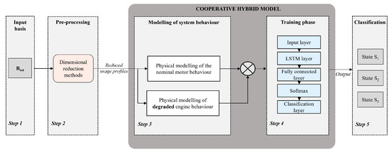
Figure 2.
Physic-augmented neural network for a motor diagnosis task.
represents the system modeling depending on the usage profile . is the physical modeling computed from the motor equations with healthy behavior . The behavior can, for example, be determined using several operating points or operating equations. The final modeling of the system is obtained by exploiting the residuals (deviation between the healthy behavior and the real system) as input data for the recurrent neural network (RNN) (Equation (2)).
3. CL Strategy Proposed
3.1. Problem Formulation
Given that usage profiles of complex systems vary over time, the constructed predictive method must be capable of reusing previously acquired and validated knowledge. This translates to enhancing the model’s generalization capabilities when encountering new profiles. Indeed, the limitation of data-driven approaches is that they do not guarantee their proper functioning in situations not included in the database used to train the models. Thus, the issue lies in managing the progressive arrival of data with control over the model’s convergence. The contribution made since the previous work pertains to the preprocessing stage (see step 2 in Figure 3) and the training phase (step 3 in Figure 3). The preprocessing stage is based on the reduction methods previously tested. One of the first solutions considered is the foundation of initial learning on reduced bases while retaining useful information. The bases before reduction contain the usage profiles that the system may encounter. By eliminating redundancies, the model has an easier time generalizing its prediction performances in the face of unknown profiles. This reduces the risks of model divergence. It is therefore an optimization between reducing the number of usage profiles and increasing variability in the data. The methodology presented primarily focuses on preprocessing the bases containing usage profiles.
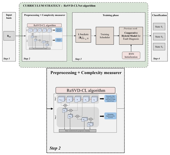
Figure 3.
Framework of the global methodology proposed with the training. Zoom on the second Step of the method.
The second part is built on the concept of curriculum learning. The task is to develop a complexity measuring tool and a training schedule that can suggest a personalised curriculum strategy for temporal signals. Our strategy belongs to the automatic CL category, as it combines signal processing knowledge with a reliance on data-driven models. Regarding scheduling, it gradually retrieves unique modes. Due to this design, the obtained training bins will be unevenly divided, unlike most predefined curriculum methods in the literature. The implemented training scheduler belongs in this case to discrete schedulers. Kocmi [80] notably studied the effect of this sampling category by modifying the Baby-Step Curriculum Learning (BS-CL). The Cooperative Hybrid Model has the same structure as shown in Figure 2.
3.2. Dataset
The input data we focus on are the input commands sent to the physical model (see step 1 in Figure 3). These data consist of periodic time series and constitute a database of speed profiles, . The residual physical data obtained after step 3 (Figure 3) is referred to as the output data. For the purpose of this study, the input speed profiles () are divided into 4 initial bases depending on the shape of the signal and the frequency range to which it belongs. This choice of four buckets was made to cover a representative diversity of usage profiles typically encountered in electric motor systems, including low- and high-frequency sinusoidal and pulse waveforms. However, this structure is not restrictive: the ReSVD-CL framework is designed to accommodate the straightforward integration of new bases as new usage scenarios emerge.
The 4 bases, each comprising 90 signals with frequencies ranging from 1 Hertz to 100 Hertz, are called buckets. The bases differ by frequency, which progressively increases within the signals (see Figure 4).
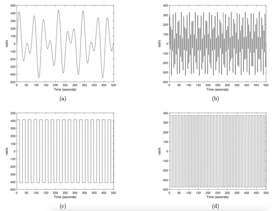
Figure 4.
Examples of velocity profiles for each base. Subfigure (a) shows a sample velocity profile of basis; subfigures (b–d) correspond to , , and , respectively.
They are ordered according to their physical characteristics, namely, their frequency and amplitude, which increase gradually. The first base contains only low-frequency sinusoidal profiles, the second base comprises higher-frequency sinusoidal profiles, the third base includes low-frequency pulse wave profiles, and the final base consists of higher-frequency pulse wave profiles. This order stems from how they were created: the model was previously tested on typical usage profiles. Subsequently, its ability to adapt to broader usage profiles was verified. This approach is representative of real-world scenarios when the system has already been modeled and is used with new usage conditions. A measure of the complexity of the bases, from the model’s perspective, is then described in Section 3.3. The predictor data are an array of cells containing residual data sequences of the same length with four features. Each sequence consists of 5000 time steps. The predictor sequences are therefore matrices with four rows (one row for each feature) and 5000 columns (one column for each time step). The target data is a categorical vector of 5000 labels, corresponding to the three possible stages of motor failure at each time step: “healthy”, “progressive failure” and “stable failure”. An 80/20 distribution is applied for the learning phase and the test phase, respectively. This means keeping 864 sequences for learning and 216 sequences for testing the model. Among the 80% of sequences reserved for the learning phase, 10% are used for the validation phase.
3.3. Complexity Measurer
In the context of time series, i.e., with a time dependency, the complexity between the initial buckets is measured based on their similarity. The criterion to be used to define the order of injection of the bases in the learning process must be capable of comparing multiple sets of signals. Indeed, if the multivariate time series base analysis is processed by decomposing it into different univariate signals or concatenated into a single time series, crucial correlations will certainly be lost. Each initial base, consisting of multiple time signals, is thus viewed in our case as a multivariate time series (MTS) of the form , where i represents a measurement at time step t. Each signal is measured from 0 to 500 s with a frequence of 10 Hz, so the signals are comparable. MTS are commonly stored in an matrix where m is the number of observations and n is the number of variables. For the remainder, we assume that m is the number of time steps (5001 in this case) and n is the number of signals present in a base. The adopted complexity measure is the Eros measure, which is an extension of the Frobenius norm. The latter is a method for calculating the norm of a matrix and is known for its ease of implementation [81]. It is hypothesized that the more similar a base is to previous bases, the less complex it is to study from the model’s perspective. As for the Eros measure, as precisely defined by Yang et al. [82], it quantifies the similarity between two matrices using principal components, namely the eigenvectors of the covariance matrices and the eigenvalues. This measure is suitable for this study due to periodic signals. Let A and B be two MTS items of size and , respectively. Let and be two right eigenvector matrices obtained by applying Singular Value Decomposition (SVD) to the covariance matrices, and , respectively. Let and . The Eros similarity measure is calculated as follows:
where is the inner product of and , w is a weight vector which is based on the eigenvalues of the MTS dataset, and is the angle between and . The range of Eros is between 0 and 1, with 1 being the most similar.
To measure the mutual similarity of the bases, we refer to the first accessible base , which contains the non-extrapolated classical profiles. and the other bases are compared based on their first 15 modes extracted via the Singular Value Decomposition (SVD) method. Indeed, a preliminary study of the energy of the modes confirmed that 15 modes were sufficient to represent at least 85% of the variability in the databases. This complexity criterion is applied in step 2 of the Figure 3. It classifies the initial bases according to their complexity before the ReSVD-CL algorithm is used to determine the residual singular modes. In cases where new bases are to be integrated into the posterior learning phase, the measure will calculate between which training steps it is advisable to place them.
3.4. Training Scheduler
Once the injection order of the bases is determined according the complexity measurer (see Section 3.5), it remains to specify the timing of injecting these bases. The injection timing is specified by the training scheduler (), hereafter referred to as the scheduling criterion. In our case, it corresponds to the convergence criterion of the loss function (step 3 in Figure 3). For a judiciously chosen number of epochs based on the number of time sequences present in each base, learning continues until the convergence criterion is reached. It represents the difference between the average of the last m terms of the loss function history and the last term of at each iteration. Thus, between each base injection, the following inequality Equation (4) must be respected:
with n being the current term of the ongoing iteration and m the number of terms chosen to ensure convergence. After optimization, we set for this study. The scheduling stops once all the training bases have been processed and the loss function has converged.
3.5. Methodology
3.5.1. Pre-Processing
This subsection corresponds to step 2 in Figure 3. The purpose of this step is to establish the relative complexity of each base in relation to the others. This categorisation determines the order in which the bases are injected into the predictive model during the training phase.
The ReSVD-CL algorithm (Residual Singular Value Decomposition Curriculum Learning), incorporating the curriculum learning principle, is divided into 3 steps described below (see Algorithm 1). Step 1 (Figure 5) involves constructing the initial profile bases and is detailed in Section 3.2. It also orders the bases according to their similarity relative to the first initial base . The similarity growth logically follows the order of base construction. The ReSVD-CLNet model (Residual Singular Value Decomposition Curriculum Learning Net) comprises the ReSVD-CL algorithm as well as the entire learning phase (see Algorithm 2). During the step 2 (Figure 5), the initialization of ReSVD-CL is done by extracting the singular values from until reaching 90% of cumulative explained variability (). It is noted that selection above 90% has been shown to encourage over-fitting when testing the model on new data, with a number of selected mode decreased by 30% for % ), while selection below 90% has been shown to encourage under-fitting, with a number of selected mode increased by more than 50% for % ). However, while this threshold proved suitable in the present context, it has to be discussed in an other as it is inherently dependent on both the diversity and the size of the data.
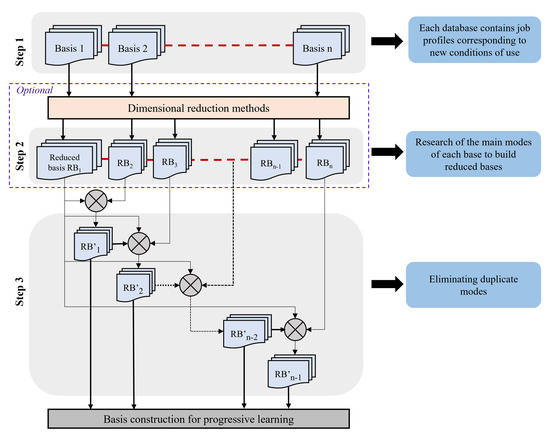
Figure 5.
ReSVD-CL Algorithm.
The resulting , , and matrices from the SVD method are stored for comparison with the other initial bases. During subsequent iterations on the remaining initial bases, new modes are retrieved while ensuring duplicate modes are eliminated. To verify this, each signal from a given base is projected onto the modes from previous iterations. This requires concatenating the modes from previous iterations, forming a new mode base . Next, the projected signal is reconstructed in the time domain and subtracted from the original time signal. If the difference between the residual signals and the original signals is too high, a new mode study via the SVD method on the obtained residual signals is reiterated. This difference is calculated through an RMSE (Root-Mean-Square Error) criterion . Considering that each base consists of 90 signals of 500 s at a sampling frequency of 10 Hz, the mean square error tolerated to confirm that the 2 bases are sufficiently well reconstructed is arbitrarily chosen to be 100. This criterion will be optimized in future works. If does not reach this threshold for a given base, no new mode is added. The new modes are finally added while respecting the criterion of cumulative explained variability. The ReSVD-CL algorithm concludes after processing the 4 initial bases. The reduced bases , output from ReSVD-CL, form the profiles used to initialize the learning of the predictive hybrid ReSVD-CLNet model.
| Algorithm 1: ReSVD-CL Algorithm |
|
The speed commands derived from the reduced bases are then applied to the simulated physical model of the engine, and the output variables are collected. These outputs are compared to those resulting from the nominal behavior of the engine and subjected to the classification model.
More specifically, in Algorithm 2, Algorithm 1 is initially applied to the entire set of B-mode signals in order to extract all unique modes (line 2). Subsequently, at each iteration, once a new singular mode has been retrieved, the set of signals S is evaluated to determine whether it satisfies criterion (line 4). If the criterion is fulfilled, the ReSVD-CLNet classification model is trained using the set of modes accumulated up to iteration i (line 6).
| Algorithm 2: ReSVD-CLNet Algorithm |
|
The methodology is described focusing on four primary bases (see Figure 4), as they are sufficient to cover the various types of profiles that our electric motor may encounter. The scenario where new operating conditions are identified at the end of the training is addressed in Section 3.6.
3.5.2. Training Process
Since the input data consists of temporal sequences, the suitable black-box model is a recurrent neural network. Specifically, understanding both short-term and long-term dependencies is crucial for detecting deviations in the motor behavior. The LSTM network is naturally chosen to meet these requirements. The effectiveness of the different learning approaches presented in this work will be evaluated using the F1-Score. This metric is commonly used for problems involving imbalanced data, as in our case. In most industrial systems, it is easier to observe healthy data than faulty data. A high F1-score, close to 1, indicates good model performance in terms of precision and recall. It is calculated by combining precision and recall. Precision summarizes the proportion of true positive predictions made by the model among all instances predicted as positive. Recall measures the proportion of true positive predictions made by the model among all actual positive instances. Since this is a multi-class problem, the final -Score was obtained by averaging the F1-Score of each class c (“progressive wear”, “stabilized wear” and “healthy state”).
Remark: In general, for the test cases considered in this work, the “healthy state” class exhibits the highest precision and recall, while “stabilized wear” shows the lowest precision. As an example, for a final F1-score of 0.917, the obtained values are given in Table 1

Table 1.
F1-Score, recall and precision for each classes with the use of SVD in the reduction step.
Once the preprocessing is finished, the learning phase begins. It is divided into 2 main distinct periods: learning, performed exclusively on each of the buckets, and , applied according to the ReSVD-CLNet model (see Figure 6). The global training is used to build four predictive model structures, each trained on a single bucket. In the context of diagnosing a novel base, the objective is to evaluate the diagnostic efficacy of a model that has been trained on multiple bases, in comparison to a model that has been specifically trained on a base that is analogous to the new base. The training is performed by merging the previous training bases with the active base. This way, a certain distribution between iterations is maintained to ensure the stability of the learning convergence. When integrating a new base by the training scheduler, all weights obtained at the end of the previous phase are transferred as initialization of the network at the beginning of the next training phase. Early stopping is also implemented if the loss does not improve for a chosen number p of epochs. Given the challenge of generalising the input data without retraining the model, is expected to converge much faster than . However, is expected to perform better in F1-score on new data. This intuition will be confirmed in Section 4.2.
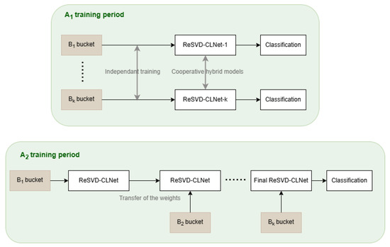
Figure 6.
Illustration of the two main training phases: (independent learning on each ) and (progressive training via weight transfer across buckets).
3.6. Management Loop for Loss of Information
The primary objective of this work is to ensure extrapolation capabilities by reducing the amount of input data. This involves a trade-off between the quantity of reduced data and the quality of the reduction during the preprocessing phase namely the projection on the reduced bases. Once the compromise is accepted, the RNN is initialized with the input buckets. An initial assessment is conducted by quantifying the variability retained in each input bucket compared to the originally available data. This assessment is confirmed with the F1-Score values.
However, when the model is fed with new real data from the engine, this can vary significantly from the training data. This can be checked by identifying new usage profiles and injecting them into the ReSVD-CL algorithm. If is satisfied, the RNN initialization is sufficient to diagnose the new output data without re-training the model. In cases where is not satisfied, reinforcement of the RNN is initiated by learning . Secondary buckets are thus created after passing through the ReSVD-CL algorithm. They will be used as training data for another refined model of the ReSVD-CLNet type (RNN Reinforcement part in Figure 7). In addition, the weights of the RNN initialised with the primary buckets are not overwritten. In fact, it is considered to be the teaching network. As for the RNN trained with the secondary buckets, it is considered to be the student network. This approach makes it possible to maintain the performance of each structure, offering flexibility in their use according to the different use cases.
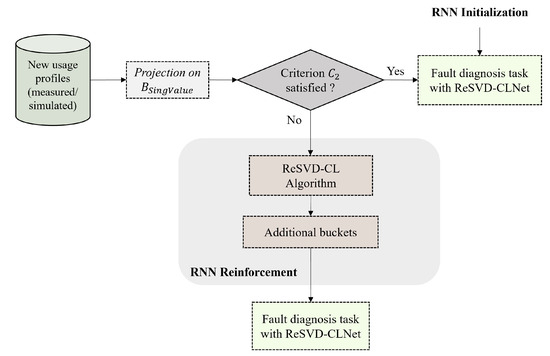
Figure 7.
Flowchart for managing a new bucket.
4. Experiments and Testing Results
In the following, the proposed method is evaluated using four bases of speed profiles. and consist of sinusoidal signals with progressively increasing amplitude and frequency ranges, while and are composed of impulse waveforms with similar range variations. A representative example from each primary base is illustrated in Figure 4.
4.1. Training Performances
To validate the management of the intermittent arrival of profile bases into the model, the convergence capabilities are tested during different stages of learning. The curriculum learning strategy is thus compared to the model without the grafting of the ReSVD-CL algorithm. If the full set of possible velocity profiles is known at the outset, the model will have more data to work with at the outset. Clearly, it will be easier to establish correlations and generalize the training data to new data. Classification performance will then be superior compared to that of the ReSVD-CLNet. However, in our problem of generalization and extrapolation of usage profiles, the implemented curriculum learning seems appropriate where unknown profiles can randomly appear.
In Figure 8, the loss function displayed at each iteration demonstrates that the more the active learning base differs from , the more iterations the process requires to reach the convergence criterion. The learning steps were stopped before reaching the maximum fixed epochs. In this particular instance, it is imperative to acknowledge that the maximum number of epochs is determined in accordance with the number of signals present within the training databases.The curriculum strategy, constructed with the objective of attaining the optimal reduction of input data, results in a paucity of data following pre-processing. This renders the model susceptible to the overfitting problem. The selection of the number of epochs serves to circumvent this issue to a certain extent. However, it is imperative to note that the number of epochs must increase in parallel with the number of buckets merged, thereby ensuring the condition of increasing accuracy in the optimisation of the algorithm. According to the similarity criterion of the initial buckets, is very similar to (eros similarity = 0.38). Consequently, step 2 converges very quickly even if the expected optimization is more demanding than at step 1. and are similar to each other (eros similarity = 0.15) but less similar to . Although convergence thus requires more iterations, the loss function continues to decrease. The learning phase is then considered successful (Table 2).
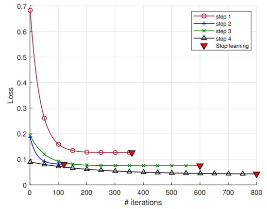
Figure 8.
Learning stages of the ReSVD-CLNet. The loss was smoothed with a non-linear fit of exponential decay model.
Table 2.
Accuracy rate at each learning stage of the ReSVD-CLNet.
4.2. Testing Performances
The testing phase serves, on the one hand, to assess the predictive model’s generalization capabilities when facing new data. On the other hand, we will evaluate the relevance of the implemented curriculum learning strategy by verifying that the classification performances are higher than before. For this purpose, a set of 3 test bases each containing 90 modified speed profiles is created. They randomly contain sinusoidal profiles and impulse waves. They are intentionally constructed to resemble different initial bases. After calculating their similarity, is more similar to , to , and to . Table 3 illustrate the variability between the test bases and the initial ones, expressed as a percentage. It can be observed that the test bases exhibit high variability, highlighting their dissimilarity with the training data and thereby supporting their relevance for evaluating extrapolation capabilities.
Table 3.
Percentage variability of test bases compared to initial bases. “Mag.” is for the magnitude variability and “Freq.” for the frequency variability.
The bases undergo preprocessing initially to conform to the data format seen during training. Specifically, each of the bases is projected onto the space of unique modes derived from the 4 primary bases and recorded in (where corresponds to the last iteration). After projection, they are reconstructed in the temporal domain to fit the type of input data for the motor’s physical model. Then, they undergo random perturbations, and the output data is retrieved. They are compared to the base containing multiple identifications of the nominal behavior of the engine to form residual data. Finally, the data is classified according to the 4 different recurrent model structures obtained during the detailed training phase outlined above. These structures then incorporate the entirety of the curriculum learning process.
The F1-Scores depicted in Figure 9 show that the classification performance continues to improve throughout the learning process. This validates firstly that the curriculum learning strategy, as well as the difficulty measurer and the training scheduler, are relevant for our use case. Indeed, even if a base is very similar to one of the initial bases included in , defects are better detected with the RNN structure obtained at the end of training with the ReSVD-CL algorithm. Similarly, the classification performance for a new test base is higher with the ReSVD-CLNet-4 model than with the model trained solely on the most similar base.
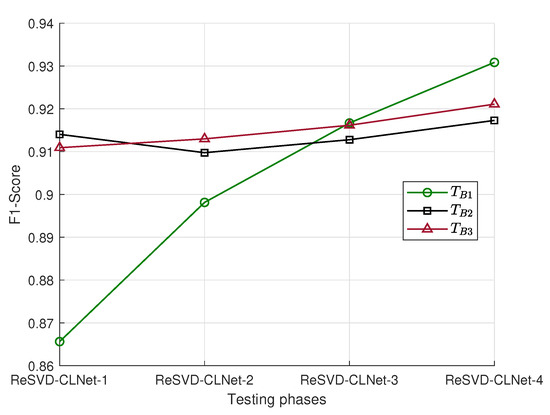
Figure 9.
Testing of the different model structures obtained between each training step.
4.3. Influence of the Difficulty Measurer
To validate the complexity measure based on similarity, the injection order of the bases is modified while keeping the ReSVD-CL algorithm. This results in unsorted buckets from easiest to hardest. Since this no longer adheres to the CL concept, this regimen will be referred to as No-Curriculum Learning (No-CL) later. Several injection orders are compared. To compare the regimens, the selected order is the one that ensured the lowest similarity between the bases. The learning recorded under these conditions is denoted as .
5. Comparison with Existing Regimens
After demonstrating that the ReSVD-CL algorithm was suitable for preprocessing the input data, it is necessary to validate the applicability and superiority of the proposed CL strategy. For comparison purposes, commonly employed regimens in the literature are set up to evaluate the same dataset. They all incorporate the ReSVD-CL algorithm as well as the characteristics of curriculum learning for a fair comparison. This implies that the buckets are sorted in the same way as before. The first regimen is the One-Pass curriculum originally proposed by Bengio et al. [51], and the second one is the Baby Step curriculum from Spitkovsky, Alshawi, and Jurafsky [83]. Through the formalization of concepts in [84] on a sentiment analysis task, a comparison of the algorithmic advantages could be observed. Additionally, the proposed approach will be evaluated against state-of-the-art models.
5.1. One-Pass CL
After sorting from the easiest bucket to the most difficult one, the One-Pass curriculum learning (OP-CL) gets its name from the single-pass learning mode. The process, described by [51], processes the buckets one by one, and the model encounters them only once during training. In practice, it trains on the first instance until convergence after a certain number of epochs p. This first bucket is then set aside for the remainder of the training. Subsequently, training continues by injecting the second bucket, deemed more difficult. Training concludes once all the buckets have been studied. The principle behind this algorithm is that once the model has learned from simple batches, it is capable of handling more complex batches for the same task.
Figure 10 and Table 4 demonstrate that the CL strategy is not suitable at all. Firstly, even after ordering the bases according to their similarity, the loss is higher at the end of training than with the first batch of data trained for only 100 iterations. Secondly, no instance reaches the convergence criterion for the predefined number of epochs p. In this case, the stopping criterion indicated is based on when the loss begins to increase. This stems from the lack of distribution between each bucket, further hindering the stability of the model if the buckets differ from those encountered in previous iterations. This result logically aligns with the type of input data. For example, let’s consider batch 1 containing only sinusoidal profiles and batch 2 containing pulse signals. During the first instance, the weights adjusted for batch 1 are not suitable for batch 2. When batch 1 is eliminated, optimizing new weights for batch 2 becomes complex. Indeed, for the classification task where deviations in the time signal need to be located, the deviation of a square wave differs from that of a sinusoidal wave.
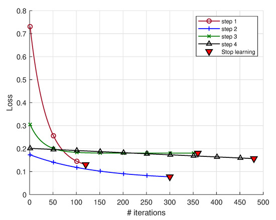
Figure 10.
Learning stages of the OP-CL.
Table 4.
Accuracy rate at each phase of training with the OP regimen.
5.2. Baby-Step CL
Unlike the One-pass approach, the simplest batches in the training data should not be discarded between each iteration. Training starts with the easiest bucket. To move to the next step, the previously used bucket and the current bucket are merged. The entire training process with the baby step CL strategy stops when all buckets have been used.
For an equal amount of data during the training period, the criterion is satisfied in very few iterations with this algorithm (see Figure 11). However, the improvement capabilities are limited. Adding batches of data does not reduce the loss. The same applies to precision, which stagnates at 85% from the second bucket onwards and does not change until the end of training. In order to enhance the model’s generalization performance, the BS-CL approach proves to be limited.
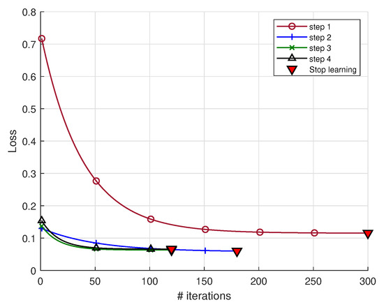
Figure 11.
Learning stages of the BS-CL.
5.3. Baseline Approaches
The ReSVD-CLNet framework is now compared to the baseline techniques in fault diagnosis with LSTM and CNN using the dataset described in Section 3.2 with the hyperparameters of the literature. The initial model is the ATT-1D CNN-GRU [85] which is a serial concatenation of 1D CNN and Gated Recurrent Unit (GRU) layers, in conjunction with an attention mechanism, applied for the rolling bearing fault diagnosis. The second model is employed for the fault diagnosis of wind turbines and is designated as the adaptive multivariate time-series convolutional network (AdaMTCN) [86]. It is built with a multi-time-step resampling layer, a basic Multivariate Time Series Convolutional Network (MTCN) model, and an adaptive decision fusion. MTCN is a CNN with a Spatial Pyramid Pooling (SPP) layer to perform pooling at different scales. The third model relevant for comparison is a combination of CNN and a LSTM layer for fault diagnosis in a chemical process [87] with multivariate time series. The F1-Score of the ReSVD-CLNet framework and the three models are compared in Section 6. In general, a substantial enhancement in performance is observed when comparing all of the proposed CL-based frameworks with the baseline techniques.
6. Results and Discussions
6.1. Results
Once a comparison of the various CL regimens has been made based on their training phase, it is imperative to analyse their behaviour when confronted with new data. Regimens are consequently evaluated based on their classification performance by reusing the test bases . In order to adhere to the CL concept, the parameters of the naturally selected models are those obtained at the conclusion of the training phase, even if the observed loss is higher.
The classification performance of different curriculum learning (CL) regimens was evaluated on the three test bases (), using models with parameters obtained at the end of their respective training phases. The results, summarised in Table 5, reveal notable differences in performance across regimens, particularly in terms of the F1-score. Among the approaches evaluated, ReSVD-CL demonstrated the highest level of performance, with F1-scores of 0.870, 0.835, and 0.850 on the three test sets. This finding suggests that the SVD-based preprocessing enhances the model’s capacity for generalisation to new data. The BS-CL approach also demonstrated commendable performance, albeit with marginally lower scores (0.829, 0.748, and 0.781), suggesting that its curriculum strategy is indeed efficacious, though it may not capture certain key features with the same proficiency as ReSVD-CL. In contrast, the OP-CL demonstrated moderate performance, with F1-scores ranging from 0.550 to 0.596. This suggests that, while benefiting from a structured learning approach, OP-CL is less effective than both BS-CL and ReSVD-CL. The No-CL regimen, which lacks curriculum learning, yielded the lowest performance, with scores ranging from 0.297 to 0.300, thus highlighting the importance of curriculum-based strategies for classification tasks.
Table 5.
Classification performance with different CL regimens and baseline approaches on the 3 test bases.
Subsequently, a comparative analysis of the performance of the ReSVD-CL framework with other fault diagnosis models from the literature is conducted, with a particular focus on recent models such as ATT-1D CNN GRU, AdaMTCN, and CNN-LSTM, in order to evaluate its generalisation capabilities. The ATT-1D CNN GRU model, with F1-scores of 0.644, 0.561, and 0.596, demonstrates enhancement over AdaMTCN and CNN-LSTM, yet remains inferior to the ReSVD-CL framework. AdaMTCN and CNN-LSTM demonstrate significantly lower performance, with F1-scores of 0.322, 0.317, and 0.322 for AdaMTCN, and 0.365, 0.361, and 0.370 for CNN-LSTM, indicating their limited generalisation capability. The BS-CL model performs better than ATT-1D CNN GRU, AdaMTCN, and CNN-LSTM, yet still trails behind ReSVD-CL in terms of F1-score. In conclusion, the ReSVD-CL framework outperforms ATT-1D CNN GRU, AdaMTCN, CNN-LSTM, and other CL regimens such as OP-CL and BS-CL.
As shown in Table 5, while lightweight models such as AdaMTCN (0.3 min) and ATT-1D CNN GRU (0.8 min) exhibit shorter per-iteration durations, they require a greater number of iterations to reach convergence. In contrast, ReSVD-CL maintains an iteration time of 2.5 min, reflecting its efficiency and robustness. Notably, No-CL presents the longest iteration time (4.1 min) with the poorest performance, highlighting the value of structured training regimens.
6.2. Discussions
The results of this study demonstrate the potential of the ReSVD-CLNet framework to improve generalisation performance through structured profile selection and curriculum-based training. The methodology performed effectively when applied to a set of well-characterised faults within a clearly defined use case, thereby confirming its ability to balance model complexity and data variability. The choice to retain 90% of the variance following dimensionality reduction was informed by the characteristics of the dataset. While this threshold proved suitable in the present context, it is inherently dependent on both the diversity and the size of the data. Retaining too few profiles may result in underfitting, whereas retaining too many could lead to overfitting, each of which can impair the model’s ability to generalise. A key strength of the proposed approach lies in its capacity to manage information loss and to support model selection as new data profiles become available. This is particularly advantageous in applications where datasets are subject to variation or progressive evolution. Nonetheless, a notable limitation of this study is the exclusive reliance on simulated signals. Although simulations facilitate controlled experimentation and enhance reproducibility, they may not fully capture the complexities or uncertainties associated with real-world data. Future work should therefore include validation using physical experiments to assess the practical applicability of the method under realistic conditions.
An additional consideration concerns the effort required to define CL features. In domains where expert knowledge is limited or difficult to obtain, the manual specification of CL criteria may be time-consuming and subjective. In such cases, automated CL strategies offer a promising alternative to reduce reliance on expert input whilst maintaining training efficiency. Although the approach has been validated in a specific context, it remains adaptable to other application areas (e.g., automation, structural design), provided that appropriate complexity measures and training schedules are defined. Indeed, the workflow will remain the same but the nature of the input data and its main characteristics have to be taken into account in the choice of the CL method functions and parameters. It should also be noted that the application of this methodology may not always be necessary. In well-defined settings with stable data distributions, conventional techniques or pre-trained models may suffice, rendering profile-based SVD analysis superfluous. A worthwhile avenue for future research would be to determine the degree of divergence between the source and target data distributions at which the application of transfer learning becomes justified. Such a study would contribute to a more principled framework for selecting the most appropriate modelling strategy based on the available data and domain knowledge.
7. Conclusions
This study investigates the efficacy of CL strategies in enhancing classification performance, with ReSVD-CL proving to be the most effective approach. By integrating a CL strategy with SVD-based dimensionality reduction, ReSVD-CL demonstrates enhanced model generalisation, surpassing alternative regimens such as BS-CL, OP-CL, and No-CL. The findings of this study substantiate the notion that the amalgamation of structured learning and dimensionality reduction leads to a substantial enhancement in model accuracy, particularly in scenarios that necessitate extrapolation to novel data distributions. The proposed methodology capitalises on the salient characteristics of the data (e.g., temporal dependence, periodicity), yet it is the distinctive attributes of the ReSVD-CL strategy (e.g., Eros similarity, the training scheduler, and the SVD-based method) that substantially enhance the classification performance. By methodically introducing data batches of increasing complexity according to Eros, this approach not only stabilises the training process but also enhances the generalisability to novel usage profiles. Furthermore, the hybrid model enables continuous adaptation, accommodating new usage conditions without necessitating complete retraining.
Overall, this work highlights the advantages of combining curriculum learning with traditional input dimension reduction techniques, reducing computational costs while accelerating model convergence. The findings suggest that adaptive CL-based approaches offer a promising avenue for enhancing classification models in dynamic and evolving environments. A significant limitation of extant CL methods in the literature is their rigidity, as predefined dataset partitions and pacing functions restrict adaptability [88]. In contrast, the proposed strategy introduces a dynamic learning framework capable of continuous refinement as new conditions arise. This adaptability reduces training data requirements while ensuring high diagnostic performance across a broader range of scenarios. Beyond improving extrapolation, this approach enhances diagnostic performance compared to specialised models. Future numerical work will concentrate on the refinement of information loss management and the optimisation of model architecture selection for evolving profiles. In parallel, an experimental work will be conducted to test the proposed approach in the case of an electrical motor of a linear axis for machining. In this work, velocity, voltage, current, and position will be recorded, and the resulting time series will be used to validate the proposed methodology. The impact of noise on data reduction and potential information loss will also be analyzed.
The integration of automated CL strategies has the potential to further enhance efficiency, particularly in domains where domain knowledge is insufficient for defining complexity measures. In addition, this methodology is currently being validated on real-world data on a test bench to assess its practical applicability and performance in dynamic environments.
Author Contributions
Conceptualization, M.S., E.A.-C. and P.-A.R.; methodology, M.S., E.A.-C. and P.-A.R.; software, M.S.; validation, M.S. and E.A.-C.; formal analysis, M.S.; investigation, M.S. and E.A.-C.; resources, M.S. and E.A.-C.; data curation, M.S.; writing—original draft preparation, M.S.; writing—review and editing, M.S. and E.A.-C.; visualization, M.S., E.A.-C. and P.-A.R.; supervision, E.A.-C. and P.-A.R.; project administration, E.A.-C.; funding acquisition, E.A.-C. All authors have read and agreed to the published version of the manuscript.
Funding
This research was funded by Région Nouvelle Aquitaine with the SABOR Project.
Data Availability Statement
The raw data supporting the conclusions of this article will be made available by the authors on request.
Conflicts of Interest
The authors declare no conflicts of interest.
References
- Liu, G.; Shen, W.; Gao, L.; Kusiak, A. Predictive modeling with an adaptive unsupervised broad transfer algorithm. IEEE Trans. Instrum. Meas. 2021, 70, 1–12. [Google Scholar] [CrossRef]
- Luo, S.; Huang, X.; Wang, Y.; Luo, R.; Zhou, Q. Transfer learning based on improved stacked autoencoder for bearing fault diagnosis. Knowl.-Based Syst. 2022, 256, 109846. [Google Scholar] [CrossRef]
- Zhu, Z.; Lei, Y.; Qi, G.; Chai, Y.; Mazur, N.; An, Y.; Huang, X. A review of the application of deep learning in intelligent fault diagnosis of rotating machinery. Measurement 2023, 206, 112346. [Google Scholar] [CrossRef]
- Eren, L.; Ince, T.; Kiranyaz, S. A generic intelligent bearing fault diagnosis system using compact adaptive 1D CNN classifier. J. Signal Process. Syst. 2019, 91, 179–189. [Google Scholar] [CrossRef]
- Schwendemann, S.; Amjad, Z.; Sikora, A. Bearing fault diagnosis with intermediate domain based layered maximum mean discrepancy: A new transfer learning approach. Eng. Appl. Artif. Intell. 2021, 105, 104415. [Google Scholar] [CrossRef]
- Asutkar, S.; Tallur, S. Deep transfer learning strategy for efficient domain generalisation in machine fault diagnosis. Sci. Rep. 2023, 13, 6607. [Google Scholar] [CrossRef] [PubMed]
- Estrada-Flores, S.; Merts, I.; De Ketelaere, B.; Lammertyn, J. Development and validation of “grey-box” models for refrigeration applications: A review of key concepts. Int. J. Refrig. 2006, 29, 931–946. [Google Scholar] [CrossRef]
- Rajulapati, L.; Chinta, S.; Shyamala, B.; Rengaswamy, R. Integration of machine learning and first principles models. AIChE J. 2022, 68, e17715. [Google Scholar] [CrossRef]
- Zendehboudi, S.; Rezaei, N.; Lohi, A. Applications of hybrid models in chemical, petroleum, and energy systems: A systematic review. Appl. Energy 2018, 228, 2539–2566. [Google Scholar] [CrossRef]
- Quiza, R.; López-Armas, O.; Davim, J.P. Hybrid Modeling and Optimization of Manufacturing: Combining Artificial Intelligence and Finite Element Method; Springer Science & Business Media: Berlin/Heidelberg, Germany, 2012. [Google Scholar]
- Sun, W.; Yan, R.; Jin, R.; Zhao, R.; Chen, Z. Curriculum-Based Federated Learning for Machine Fault Diagnosis with Noisy Labels. IEEE Trans. Ind. Inform. 2024, 20, 13820–13830. [Google Scholar] [CrossRef]
- Zhang, K.; Wang, B.; Zheng, Q.; Ding, G.; Ma, J.; Tang, B. A novel fault diagnosis of high-speed train axle box bearings with adaptive curriculum self-paced learning under noisy labels. Struct. Health Monit. 2025. [Google Scholar] [CrossRef]
- Lai, P.; Zhang, F.; Li, T.; Guo, J.; Teng, F.; Liu, R. A Curriculum-Based Meta-Learning Approach for Few-Shot Fault Diagnosis. In Proceedings of the 2023 3rd International Conference on Digital Society and Intelligent Systems (DSInS), Chengdu, China, 10–12 November 2023; IEEE: Piscataway, NJ, USA, 2023; pp. 224–229. [Google Scholar]
- Wang, Z.; Xuan, J.; Shi, T. Multi-label fault recognition framework using deep reinforcement learning and curriculum learning mechanism. Adv. Eng. Inform. 2022, 54, 101773. [Google Scholar] [CrossRef]
- de Las Morenas, J.; Moya-Fernández, F.; López-Gómez, J.A. The edge application of machine learning techniques for fault diagnosis in electrical machines. Sensors 2023, 23, 2649. [Google Scholar] [CrossRef]
- Alwodai, A.; Gu, F.; Ball, A. A comparison of different techniques for induction motor rotor fault diagnosis. J. Physics Conf. Ser. 2012, 364, 012066. [Google Scholar] [CrossRef]
- Jigyasu, R.; Sharma, A.; Mathew, L.; Chatterji, S. A review of condition monitoring and fault diagnosis methods for induction motor. In Proceedings of the 2018 Second International Conference on Intelligent Computing and Control Systems (ICICCS), Madurai, India, 14–15 June 2018; IEEE: Piscataway, NJ, USA, 2018; pp. 1713–1721. [Google Scholar]
- Mallioris, P.; Aivazidou, E.; Bechtsis, D. Predictive maintenance in Industry 4.0: A systematic multi-sector mapping. CIRP J. Manuf. Sci. Technol. 2024, 50, 80–103. [Google Scholar] [CrossRef]
- Morhain, A.; Mba, D. Bearing defect diagnosis and acoustic emission. Inst. Mech. Eng. Part J. Eng. Tribol. 2003, 217, 257–272. [Google Scholar] [CrossRef]
- Al-Ghamd, A.M.; Mba, D. A comparative experimental study on the use of acoustic emission and vibration analysis for bearing defect identification and estimation of defect size. Mech. Syst. Signal Process. 2006, 20, 1537–1571. [Google Scholar] [CrossRef]
- Li, C.J.; Li, S. Acoustic emission analysis for bearing condition monitoring. Wear 1995, 185, 67–74. [Google Scholar] [CrossRef]
- Tandon, N.; Yadava, G.; Ramakrishna, K. A comparison of some condition monitoring techniques for the detection of defect in induction motor ball bearings. Mech. Syst. Signal Process. 2007, 21, 244–256. [Google Scholar] [CrossRef]
- Govardhan, T.; Choudhury, A.; Paliwal, D. Vibration analysis of a rolling element bearing with localized defect under dynamic radial load. J. Vib. Eng. Technol. 2017, 5, 165–175. [Google Scholar]
- Fontes, A.S.; Cardoso, C.A.; Oliveira, L.P. Comparison of techniques based on current signature analysis to fault detection and diagnosis in induction electrical motors. In Proceedings of the 2016 Electrical Engineering Conference (EECon), Colombo, Sri Lanka, 15 December 2016; IEEE: Piscataway, NJ, USA, 2016; pp. 74–79. [Google Scholar]
- Junior, R.F.R.; dos Santos Areias, I.A.; Gomes, G.F. Fault detection and diagnosis using vibration signal analysis in frequency domain for electric motors considering different real fault types. Sens. Rev. 2021, 41, 311–319. [Google Scholar] [CrossRef]
- Tahmasbi, D.; Shirali, H.; Souq, S.S.M.N.; Eslampanah, M. Diagnosis and root cause analysis of bearing failure using vibration analysis techniques. Eng. Fail. Anal. 2024, 158, 107954. [Google Scholar] [CrossRef]
- Fatima, S.; Mohanty, A.; Kazmi, H. Fault classification and detection in a rotor bearing rig. J. Vib. Eng. Technol. 2016, 4, 491–498. [Google Scholar]
- Li, H.; Zhang, Y. Bearing faults diagnosis based on EMD and Wigner-Ville distribution. In Proceedings of the 2006 6th World Congress on Intelligent Control and Automation, Dalian, China, 21–23 June 2006; IEEE: Piscataway, NJ, USA, 2006; Volume 2, pp. 5447–5451. [Google Scholar]
- Kankar, P.K.; Sharma, S.C.; Harsha, S.P. Rolling element bearing fault diagnosis using wavelet transform. Neurocomputing 2011, 74, 1638–1645. [Google Scholar] [CrossRef]
- Sunal, C.E.; Dyo, V.; Velisavljevic, V. Review of machine learning based fault detection for centrifugal pump induction motors. IEEE Access 2022, 10, 71344–71355. [Google Scholar] [CrossRef]
- Gundewar, S.K.; Kane, P.V. Condition monitoring and fault diagnosis of induction motor. J. Vib. Eng. Technol. 2021, 9, 643–674. [Google Scholar] [CrossRef]
- Lee, D.; Siu, V.; Cruz, R.; Yetman, C. Convolutional neural net and bearing fault analysis. In Proceedings of the International Conference on Data Science (ICDATA), The Steering Committee of The World Congress in Computer Science, Computer Engineering and Applied Computing (WorldComp), Bordeaux, France, 2016; p. 194. Available online: https://worldcomp-proceedings.com/proc/p2016/DMI8005.pdf (accessed on 14 October 2025).
- Kiral, Z.; Yigit, A.; GÜRSES, B. Analysis of rolling element bearing faults via curve length transform. J. Vib. Eng. Technol. 2014, 2. [Google Scholar]
- Patidar, S.; Soni, P.K. An overview on vibration analysis techniques for the diagnosis of rolling element bearing faults. Int. J. Eng. Trends Technol. (IJETT) 2013, 4, 1804–1809. [Google Scholar]
- Mohd Ghazali, M.H.; Rahiman, W. Vibration analysis for machine monitoring and diagnosis: A systematic review. Shock Vib. 2021, 2021, 9469318. [Google Scholar] [CrossRef]
- Tama, B.A.; Vania, M.; Lee, S.; Lim, S. Recent advances in the application of deep learning for fault diagnosis of rotating machinery using vibration signals. Artif. Intell. Rev. 2023, 56, 4667–4709. [Google Scholar] [CrossRef]
- Akbar, S.; Vaimann, T.; Asad, B.; Kallaste, A.; Sardar, M.U.; Kudelina, K. State-of-the-art techniques for fault diagnosis in electrical machines: Advancements and future directions. Energies 2023, 16, 6345. [Google Scholar] [CrossRef]
- Antonino-Daviu, J.A.; Zamudio-Ramirez, I.; Osornio-Rios, R.A.; Dunai, L. Fault diagnosis in electric motors through the analysis of currents and stray fluxes. In Proceedings of the 2023 International Conference on Electromechanical and Energy Systems (SIELMEN), Craiova, Romania, 11–13 October 2023; IEEE: Piscataway, NJ, USA, 2023; pp. 1–7. [Google Scholar]
- Wang, J.; Li, Y.; Gao, R.X.; Zhang, F. Hybrid physics-based and data-driven models for smart manufacturing: Modelling, simulation, and explainability. J. Manuf. Syst. 2022, 63, 381–391. [Google Scholar] [CrossRef]
- Hanachi, H.; Yu, W.; Kim, I.Y.; Liu, J.; Mechefske, C.K. Hybrid data-driven physics-based model fusion framework for tool wear prediction. Int. J. Adv. Manuf. Technol. 2019, 101, 2861–2872. [Google Scholar] [CrossRef]
- Bhutani, N.; Rangaiah, G.P.; Ray, A.K. First-principles, data-based, and hybrid modeling and optimization of an industrial hydrocracking unit. Ind. Eng. Chem. Res. 2006, 45, 7807–7816. [Google Scholar] [CrossRef]
- Guo, F.; Li, A.; Yue, B.; Xiao, Z.; Xiao, F.; Yan, R.; Li, A.; Lv, Y.; Su, B. Improving the out-of-sample generalization ability of data-driven chiller performance models using physics-guided neural network. Appl. Energy 2024, 354, 122190. [Google Scholar] [CrossRef]
- Huang, S.; Qin, H.; Hou, W.; Zhang, X.; Zhang, X. Generalizable Physics-Guided Convolutional Neural Network for Irregular Terrain Propagation. IEEE Trans. Antennas Propag. 2025, 73, 3975–3985. [Google Scholar] [CrossRef]
- Gallup, E.; Gallup, T.; Powell, K. Physics-guided neural networks with engineering domain knowledge for hybrid process modeling. Comput. Chem. Eng. 2023, 170, 108111. [Google Scholar] [CrossRef]
- Li, Q.; Li, X.; Chen, X.; Yao, W. PEGNN: A physics embedded graph neural network for out-of-distribution temperature field reconstruction. Int. J. Therm. Sci. 2025, 207, 109393. [Google Scholar] [CrossRef]
- Elhamod, M.; Bu, J.; Singh, C.; Redell, M.; Ghosh, A.; Podolskiy, V.; Lee, W.C.; Karpatne, A. CoPhy-PGNN: Learning physics-guided neural networks with competing loss functions for solving eigenvalue problems. ACM Trans. Intell. Syst. Technol. 2022, 13, 1–23. [Google Scholar] [CrossRef]
- Suhas, M.; Abisset-Chavanne, E.; Rey, P.A. Cooperative Hybrid Modelling and Dimensionality Reduction for a Failure Monitoring Application in Industrial Systems. Sensors 2025, 25, 1952. [Google Scholar] [CrossRef]
- Yao, D.; Liu, H.; Yang, J.; Li, X. A lightweight neural network with strong robustness for bearing fault diagnosis. Measurement 2020, 159, 107756. [Google Scholar] [CrossRef]
- Selfridge, O.G.; Sutton, R.S.; Barto, A.G. Training and Tracking in Robotics. In Proceedings of the IJCAI, Los Angeles, CA, USA, 18–23 August 1985; pp. 670–672. [Google Scholar]
- Elman, J.L. Learning and development in neural networks: The importance of starting small. Cognition 1993, 48, 71–99. [Google Scholar] [CrossRef]
- Bengio, Y.; Louradour, J.; Collobert, R.; Weston, J. Curriculum learning. In Proceedings of the 26th Annual International Conference on Machine Learning, Montreal, QC, Canada, 14–18 June 2009; pp. 41–48. [Google Scholar]
- Wang, Y.; Gao, J.; Wang, W.; Yang, X.; Du, J. Curriculum learning-based domain generalization for cross-domain fault diagnosis with category shift. Mech. Syst. Signal Process. 2024, 212, 111295. [Google Scholar] [CrossRef]
- Pathak, H.N.; Paffenroth, R. Parameter continuation methods for the optimization of deep neural networks. In Proceedings of the 2019 18th IEEE International Conference On Machine Learning And Applications (ICMLA), Boca Raton, FL, USA, 16–19 December 2019; IEEE: Piscataway, NJ, USA, 2019; pp. 1637–1643. [Google Scholar]
- Wang, L.; Xu, Z.; Stone, P.; Xiao, X. Grounded curriculum learning. arXiv 2024, arXiv:2409.19816. [Google Scholar] [CrossRef]
- Gupta, K.; Mukherjee, D.; Najjaran, H. Extending the capabilities of reinforcement learning through curriculum: A review of methods and applications. SN Comput. Sci. 2022, 3, 1–18. [Google Scholar] [CrossRef]
- Yin, Y.; Chen, Z.; Liu, G.; Yin, J.; Guo, J. Autonomous navigation of mobile robots in unknown environments using off-policy reinforcement learning with curriculum learning. Expert Syst. Appl. 2024, 247, 123202. [Google Scholar] [CrossRef]
- Gao, X.; Yang, Y.; Peng, D.; Li, S.; Tan, C.; Li, F.; Chen, T. Graph Pointer Network Based Hierarchical Curriculum Reinforcement Learning Method Solving Shuttle Tankers Scheduling Problem. Complex Syst. Model. Simul. 2024, 4, 339–352. [Google Scholar] [CrossRef]
- Saglietti, L.; Mannelli, S.; Saxe, A. An analytical theory of curriculum learning in teacher-student networks. In Advances in Neural Information Processing Systems; MIT Press: Cambridge, MA, USA, 2022; Volume 35, pp. 21113–21127. [Google Scholar]
- Soviany, P.; Ionescu, R.T.; Rota, P.; Sebe, N. Curriculum Learning: A Survey. Int. J. Comput. Vis. 2022, 130, 1526–1565. [Google Scholar] [CrossRef]
- Wang, X.; Chen, Y.; Zhu, W. A Survey on Curriculum Learning. arXiv 2020. [Google Scholar] [CrossRef]
- Shi, T.; Wu, Y.; Song, L.; Zhou, T.; Zhao, J. Efficient reinforcement finetuning via adaptive curriculum learning. arXiv 2025, arXiv:2504.05520. [Google Scholar] [CrossRef]
- Zhou, S.; Wang, J.; Meng, D.; Xin, X.; Li, Y.; Gong, Y.; Zheng, N. Deep self-paced learning for person re-identification. Pattern Recognit. 2018, 76, 739–751. [Google Scholar] [CrossRef]
- Sangineto, E.; Nabi, M.; Culibrk, D.; Sebe, N. Self paced deep learning for weakly supervised object detection. IEEE Trans. Pattern Anal. Mach. Intell. 2018, 41, 712–725. [Google Scholar] [CrossRef]
- Platanios, E.A.; Stretcu, O.; Neubig, G.; Poczos, B.; Mitchell, T.M. Competence-based curriculum learning for neural machine translation. arXiv 2019, arXiv:1903.09848. [Google Scholar] [CrossRef]
- Kumar, G.; Foster, G.; Cherry, C.; Krikun, M. Reinforcement learning based curriculum optimization for neural machine translation. arXiv 2019, arXiv:1903.00041. [Google Scholar] [CrossRef]
- Doan, T.; Monteiro, J.; Albuquerque, I.; Mazoure, B.; Durand, A.; Pineau, J.; Hjelm, R.D. On-line adaptative curriculum learning for gans. In Proceedings of the AAAI Conference on Artificial Intelligence, Honolulu, HI, USA, 27 January–1 February 2019; Volume 33, pp. 3470–3477. [Google Scholar]
- Soviany, P.; Ardei, C.; Ionescu, R.T.; Leordeanu, M. Image difficulty curriculum for generative adversarial networks (CuGAN). In Proceedings of the IEEE/CVF Winter Conference on Applications of Computer Vision, Snowmass Village, CO, USA, 1–5 March 2020; pp. 3463–3472. [Google Scholar]
- Koenecke, A.; Gajewar, A. Curriculum Learning in Deep Neural Networks for Financial Forecasting. arXiv 2019. [Google Scholar] [CrossRef]
- Bucci, M.A.; Semeraro, O.; Allauzen, A.; Chibbaro, S.; Mathelin, L. Curriculum learning for data-driven modeling of dynamical systems. Eur. Phys. J. E 2023, 46, 12. [Google Scholar] [CrossRef] [PubMed]
- Sun, C.; Li, H.; Song, M.; Cai, D.; Zhang, B.; Hong, S. Adaptive model training strategy for continuous classification of time series. Appl. Intell. 2023, 53, 18821–18839. [Google Scholar] [CrossRef]
- Chen, X.; Gupta, A. Webly supervised learning of convolutional networks. In Proceedings of the IEEE International Conference on Computer Vision, Santiago, Chile, 7–13 December 2015; pp. 1431–1439. [Google Scholar]
- Portelas, R.; Colas, C.; Weng, L.; Hofmann, K.; Oudeyer, P.Y. Automatic curriculum learning for deep rl: A short survey. arXiv 2020, arXiv:2003.04664. [Google Scholar] [CrossRef]
- Tullis, J.G.; Benjamin, A.S. On the effectiveness of self-paced learning. J. Mem. Lang. 2011, 64, 109–118. [Google Scholar] [CrossRef]
- Kumar, M.; Packer, B.; Koller, D. Self-paced learning for latent variable models. In Advances in Neural Information Processing Systems; MIT Press: Cambridge, MA, USA, 2010; Volume 23, Available online: https://proceedings.neurips.cc/paper_files/paper/2010/file/e57c6b956a6521b28495f2886ca0977a-Paper.pdf (accessed on 14 October 2025).
- Matiisen, T.; Oliver, A.; Cohen, T.; Schulman, J. Teacher–student curriculum learning. IEEE Trans. Neural Netw. Learn. Syst. 2019, 31, 3732–3740. [Google Scholar] [CrossRef]
- Hacohen, G.; Weinshall, D. On the power of curriculum learning in training deep networks. In Proceedings of the International Conference on Machine Learning, Long Beach, CA, USA, 9–15 June 2019; PMLR: New York, NY, USA, 2019; pp. 2535–2544. [Google Scholar]
- Xu, B.; Zhang, L.; Mao, Z.; Wang, Q.; Xie, H.; Zhang, Y. Curriculum learning for natural language understanding. In Proceedings of the 58th Annual Meeting of the Association for Computational Linguistics, Online, 5–10 July 2020; pp. 6095–6104. [Google Scholar]
- Zhao, M.; Wu, H.; Niu, D.; Wang, X. Reinforced curriculum learning on pre-trained neural machine translation models. In Proceedings of the AAAI Conference on Artificial Intelligence, New York, NY, USA, 7–12 February 2020; Volume 34, pp. 9652–9659. [Google Scholar]
- Graves, A.; Bellemare, M.G.; Menick, J.; Munos, R.; Kavukcuoglu, K. Automated curriculum learning for neural networks. In Proceedings of the International Conference on Machine Learning, Sydney, Australia, 6–11 August 2017; PMLR: New York, NY, USA, 2017; pp. 1311–1320. [Google Scholar]
- Kocmi, T.; Bojar, O. Curriculum learning and minibatch bucketing in neural machine translation. arXiv 2017, arXiv:1707.09533. [Google Scholar] [CrossRef]
- Moon, T.K.; Stirling, W.C. Mathematical Methods and Algorithms for Signal Processing. Prentice Hall: Upper Saddle River, NJ, USA, 2000. [Google Scholar]
- Yang, K.; Shahabi, C. A PCA-Based Similarity Measure for Multivariate Time Series; Association for Computing Machinery: New York, NY, USA, 2004; pp. 65–74. [Google Scholar] [CrossRef]
- Spitkovsky, V.I.; Alshawi, H.; Jurafsky, D. From baby steps to leapfrog: How “less is more” in unsupervised dependency parsing. In Proceedings of the Human Language Technologies: The 2010 Annual Conference of the North American Chapter of the Association for Computational Linguistics, Los Angeles, CA, USA, 2–4June 2010; pp. 751–759. [Google Scholar]
- Cirik, V.; Hovy, E.; Morency, L.P. Visualizing and Understanding Curriculum Learning for Long Short-Term Memory Networks. arXiv 2016, arXiv:1611.06204. [Google Scholar] [CrossRef]
- Liu, H.; Ma, R.; Li, D.; Yan, L.; Ma, Z. Machinery fault diagnosis based on deep learning for time series analysis and knowledge graphs. J. Signal Process. Syst. 2021, 93, 1433–1455. [Google Scholar] [CrossRef]
- Zhang, G.; Li, Y.; Zhao, Y. A novel fault diagnosis method for wind turbine based on adaptive multivariate time-series convolutional network using SCADA data. Adv. Eng. Inform. 2023, 57, 102031. [Google Scholar] [CrossRef]
- Huang, T.; Zhang, Q.; Tang, X.; Zhao, S.; Lu, X. A novel fault diagnosis method based on CNN and LSTM and its application in fault diagnosis for complex systems. Artif. Intell. Rev. 2022, 55, 1289–1315. [Google Scholar] [CrossRef]
- Wang, T.; Huang, Z.; Sun, Z.; Xi, G. Reconstruction of natural convection within an enclosure using deep neural network. Int. J. Heat Mass Transf. 2021, 164, 120626. [Google Scholar] [CrossRef]
Disclaimer/Publisher’s Note: The statements, opinions and data contained in all publications are solely those of the individual author(s) and contributor(s) and not of MDPI and/or the editor(s). MDPI and/or the editor(s) disclaim responsibility for any injury to people or property resulting from any ideas, methods, instructions or products referred to in the content. |
© 2025 by the authors. Licensee MDPI, Basel, Switzerland. This article is an open access article distributed under the terms and conditions of the Creative Commons Attribution (CC BY) license (https://creativecommons.org/licenses/by/4.0/).