Abstract
Grinding surface texture is random and feature information is weak, so it is difficult to extract effective features by deep learning network. In addition, the existing deep learning methods mostly adopt a large parameter model in grinding surface roughness recognition task, and the cost of deployment in embedded end is high. In order to solve these problems, a new lightweight network model GE-MobileNet (Ghost-ECA-MobileNetV3) is proposed. Based on MobileNetV3, a feature extractor is introduced into the shallow network part of the model to enhance the ability of the network to extract and suppress the surface texture feature and noise. At the same time, SE (Squeeze-and-Excitation) attention mechanism is replaced with ECA (Efficient Channel) attention mechanism with stronger performance. Finally, the deep network layer is removed to reduce the model size. The experimental results show that the accuracy of GE-MobileNet-based grinding surface roughness measurement model on test set is 94.97%, which is better than other networks. This study proves the effectiveness of the roughness measurement method based on GE-MobileNet.
1. Introduction
In high-tech manufacturing, the surface roughness of parts has become extremely important in design and production. As a key index to evaluate part quality [1,2,3,4], surface roughness directly affects wear resistance, tightness, corrosion resistance, and assembly precision. The arithmetic mean Ra is the most commonly used roughness parameter [5]. The traditional stylus profilometer is widely used in industry, but it is slow, low in automation, and may damage the workpiece surface [6,7]. Non-contact machine vision methods, compared with optical [8,9], electrical [10], and other methods, have advantages of low cost, wide applicability, and high reliability, making them increasingly popular for surface roughness measurement.
Most machine vision methods rely on the correlation between surface image features and roughness. Yi [11,12] et al. proposed the use of color information, including sharpness and quaternion singular value entropy, to establish a grinding surface roughness prediction model. Compared with grayscale image methods, these approaches reduce information loss and improve prediction performance. However, manually designed features are limited by human cognition and are sensitive to illumination conditions.
With the rapid development of artificial intelligence, deep learning has been widely used in surface roughness measurement. Compared with traditional machine learning, deep learning avoids manual feature extraction and offers stronger feature representation and robustness. Wang [13] et al. used CNNs with transfer learning to classify abrasive belt grain size and estimate surface roughness. EL Ghadoui [14] proposed roughness detection models based on Faster R-CNN Inception V2 and ResNet50. Shi [15] used Controlled Feature Extraction Networks on microscopic images, and Huang [16] enhanced surface features using red and green light sources with VGG16 for roughness grade recognition. However, the neural networks used in the above methods have complex structures and substantial resource overhead, making them difficult to meet the requirements of high efficiency, low cost, and high precision in machine vision measurement. Therefore, a lightweight network model is more suitable for grinding surface roughness measurement.
Lightweight networks, such as MobileNet [17], GhostNet [18], MobileViT [19], and Mobile-Former [20], reduce parameters and computational cost, making them suitable for embedded applications. However, their performance in grinding surface roughness measurement is still limited [21], due to random textures and small differences between roughness grades. Figure 1 shows that grinding surfaces of different Ra values have high texture similarity, making it difficult to determine roughness grades intuitively.
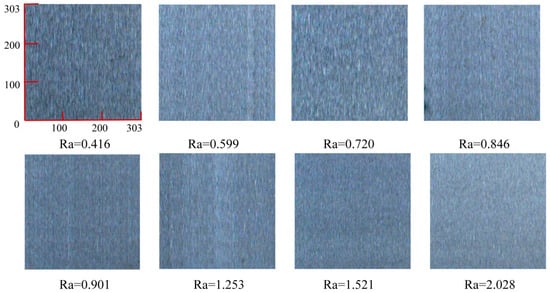
Figure 1.
Grinding surface with different roughness Ra (unit: μm); All image sizes are 303 × 303 pixels.
Fine-grained image classification, which handles large intra-class variance and small inter-class variance [22,23,24], aligns well with this task. Approaches like bilinear CNN [25], FBSD [26], and multi-CNN feature fusion [27] improve feature representation for subtle texture differences. Based on this idea, this study aims to design a lightweight network for high-precision grinding surface roughness measurement.
To enhance the feature extraction capability of the lightweight network for grinding surface roughness, GE-MobileNet is proposed as the measurement model for grinding surface roughness. First, a portion of the main network of GhostNetV2 is used as the feature extractor for MobileNetV3, sharing the shallow 3 × 3 convolution layer to reuse the extracted features. These output features are then combined with those extracted by the main network of MobileNetV3, thereby enhancing the shallow network’s ability to extract grinding surface texture features and effectively suppressing noise. Additionally, the attention mechanism in MobileNetV3 is replaced with the ECA attention mechanism. Finally, the deep network layers are removed to reduce the model’s scale. The performance of the model is evaluated through comparisons with other models. This design not only improves measurement accuracy but also enables fast, low-cost, and resource-efficient deployment in industrial grinding surface inspection systems.
2. Methods
2.1. Basic MobileNetV3
Google introduced the MobileNet series in 2017. Since then, it has become widely adopted across industry, powering a range of mobile applications such as object detection, image classification, facial attribute recognition, and face recognition. MobileNetV1 pioneered the use of depthwise separable convolutions in place of standard convolutions, dramatically cutting both computational cost and memory usage in convolutional neural networks (CNNs). Building on this, MobileNetV2 was released in 2018, featuring the inverted residual structure with linear bottlenecks, which enhanced both the depth and representational capacity of the network. In 2019, MobileNetV3 was introduced. Unlike its predecessors, it employed platform-aware NAS [28] and NetAdapt [29] to jointly search and optimize the network architecture and parameters. MobileNetV3 not only integrates the depthwise separable convolutions from V1 and the inverted residuals with linear bottlenecks from V2, but also incorporates the SE attention mechanism, enabling higher accuracy without added inference cost. Moreover, the activation function was updated from ReLU6 to h-swish, further reducing computational complexity. The overall architecture of MobileNetV3 is shown in Figure 2.

Figure 2.
MobileNetV3 structure.
Figure 3 presents the structural modules of MobileNetV3. Specifically, Figure 3a,b depict the Bneck blocks with stride values of 1 and 2, respectively. In these blocks, the first two convolutions consist of a pointwise convolution followed by a depthwise convolution, together known as depthwise separable convolutions. This design, inherited from the earlier MobileNet versions, markedly reduces computational cost and parameter usage compared with standard convolutions. The branch to the left of the main pathway represents the inverted residual structure with a linear bottleneck. To further enhance representational power, the SE attention mechanism [30] is introduced, enabling the model to better assess the importance of different feature channels. As shown in Figure 3c, the mechanism begins by applying a global average pooling layer, compressing each two-dimensional feature map into a single scalar to capture channel-wise global information. This is followed by two convolutional layers and a nonlinear activation function that establish inter-channel relationships and perform the Excitation step. Finally, a scaling operation adjusts the feature responses accordingly.

Figure 3.
MobileNetV3 related module structure. (a) MobileNetV3 Bneck structure (stride = 1); (b) MobileNetV3 Bneck structure (stride = 2); (c) SE Attention structure.
2.2. Feature Extractor GhostNetV2
Generally, shallow layers of convolutional neural networks are better at capturing fine-grained details such as color, texture, and edges due to their proximity to the input. Based on this principle, this study incorporates several Bottleneck layers from GhostNetV2 [18] into the shallow layers of MobileNetV3 as a feature extractor, thereby enhancing the model’s ability to capture the fine particle characteristics of the grinding surface. The structure of the GhostNetV2 network is shown in Figure 4. There are two key reasons for using the Bottleneck layers of GhostNetV2 as the feature extractor: first, the network architecture closely resembles that of MobileNetV3, making it easier to match the output dimensions of the network layers; second, the Bottleneck layers of GhostNetV2 integrate the DFC attention mechanism into the GhostNet layer, as depicted in Figure 5a,b. The parallel structures of the DFC attention mechanism and the Ghost module [31] enable the extraction of more abundant grinding surface features from multiple perspectives.

Figure 4.
GhostNetV2 structure.

Figure 5.
GhostNetV2 related module structure. (a) BottleNeck structure (stride = 1); (b) BottleNeck structure (stride = 2); (c) Ghost Module structure; (d) DFC Attention structure.
The Ghost module within the Bottleneck layer generates additional feature maps through inexpensive operations, effectively producing as many feature maps as a conventional convolutional layer. This enables the model to fully capture fine features related to the roughness of the grinding surface. Figure 5c demonstrates that the Ghost module extracts feature information via a 1 × 1 convolution to generate the base feature map, which is then followed by the generation of the Ghost feature map through depthwise separable convolutions of size d × d. The base feature map and the Ghost feature map are then concatenated to form the final output. The DFC attention mechanism captures long-range dependencies between pixels at different spatial positions, enhancing the model’s ability to characterize the features more effectively. As shown in Figure 5d, the DFC attention mechanism employs average pooling and dual linear interpolation for downsampling and oversampling, respectively. The horizontal FC applies a 1 × 5 convolution for horizontal operations, while the vertical FC uses the same structure.
2.3. ECA Attention Mechanism
To make the improved model more lightweight, the SE attention mechanism in the MobileNetV3 network was replaced with the ECA attention mechanism [32]. Unlike the SE module, the ECA module avoids dimensionality reduction and captures cross-channel interactions in a more efficient manner. Figure 6 illustrates the principle of the ECA attention mechanism. Compared to traditional attention mechanisms like SE, the ECA mechanism eliminates the fully connected layer after global average pooling. It instead uses a 1 × 1 convolution followed by a Sigmoid activation function to compute the channel weight values. These weight values are then element-wise multiplied with the input feature map to produce the weighted feature map as the output.
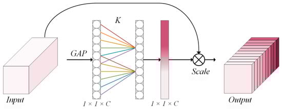
Figure 6.
ECA schematic diagram.
The attention mechanism of ECA can be represented by Formula (1). The aggregate feature is the input of the attention mechanism of ECA, represents the channel weight vector after the feature passes through the attention mechanism, represents the one-dimensional convolution, k represents the size of the convolution core of the convolution. When k = 3, the complexity of the module is the lowest and the effect is the best. denotes the sigmoid activation function.
There is a mapping relationship between the convolution kernel size k of one-dimensional convolution and the channel number C, which affects the performance of the attention mechanism to capture local channel information interaction, as shown in Formula (2):
Since the relationship characterized by the linear function is limited and the number of channels C in the neural network is usually limited to the power of 2, the mapping relationship can be expressed as a nonlinear function, as shown in Formula (3):
Therefore, the size of k can be determined according to the number of channels C, as shown in Formula (4):
where represents the nearest odd number of x, and b are set to 2 and 1, respectively.
2.4. GE-MobileNet
The classification of grinding surface roughness can be viewed as a subcategory image classification task, which requires more advanced feature extraction and more precise models to capture the subtle differences between various roughness categories. To address this, this study introduces the shallow Bottleneck layer from the GhostNetV2 network as a feature extractor into MobileNetV3, enhancing the model’s ability to extract low-level features, such as texture. To further optimize the model’s efficiency, this study replaces the SE attention mechanism in the original MobileNetV3 with the ECA attention mechanism and removes the deeper layers of the network. Based on these improvements, this study has named the resulting model Ghost-ECA-MobileNetV3, abbreviated as GE-MobileNet. The structure of the GE-MobileNet network is shown in Figure 7.

Figure 7.
GE-MobileNet structure.
The GhostNet v2 feature extractor can reuse the feature maps output by the first layer of 3 × 3 convolutional layers and extract features from another perspective and then add them to the same size features extracted by MobileNetV3. This can effectively suppress the noise of the feature maps, strengthen the extracted key features, and enhance the representation ability of the model. Compared to the method of using 1 × 1 convolutional layers for fusion after feature concatenation, the fusion method of directly adding features can save a lot of memory and time costs. The operation of introducing a feature extractor can be expressed as Formula (5), where represents the output of the input feature map x after passing through the shallow BottleNeck of MobileNetV3, represents the output of the feature map after passing through the GhostNetV2 feature extractor, represents the feature reuse operation, and y represents the weighted feature map extracted from two perspectives.
In addition, to address the issue of increasing model size caused by the introduction of feature extractors, this study removed the deep parts of the MobileNetV3 and GhostnetV2 network backbones and modified the overall network structure. Although this may weaken the model’s ability to express advanced features, it does not affect its performance in this task. Moreover, this operation can significantly reduce the number of parameters in the model. The specific structure of the GE-MobileNet network is shown in Table 1.

Table 1.
GE-MobileNet network architecture.
In Table 1, Input1 and Input2 represent the input tensor sizes for the MobileNetV3 network layer and the feature extractor layer, respectively. Operator1 and Operator2 refer to operations performed on a specific layer of MobileNetV3 and GhostNet, respectively. Bneck1 and Bneck2 represent the MobileNetV3 Bneck and GhostNetV2 Bottleneck, respectively. Expsize indicates the number of channels in the convolution of the hidden layer, and #out refers to the number of channels in the output feature map. ECA representative indicates the replacement of the network’s original attention mechanism with the ECA attention mechanism. NL denotes the type of activation function used, with this network employing ReLU and Hardswish activation functions (simplified as RE and HS in the table). Lastly, s represents the step size used in the layer convolution.
3. Experiment
The experimental flowchart is shown in Figure 8. First, the grinding sample preparation and experimental device design are completed, followed by image acquisition. The collected images are then augmented through cropping operations. Afterward, the dataset is split into a training set and a test set according to a specific ratio. The grinding surface roughness measurement model is trained using the training set, and finally, the GE-MobileNet model is evaluated using the test set.

Figure 8.
Experimental flowchart.
3.1. Sample Preparation and Workpiece Roughness
Forty-one sample blocks were processed using a regular surface grinder (M7150H), with dimensions of 50 × 50 × 10 mm and made of 45# steel. The grinding machine is shown in Figure 9, with the workpiece fixed using a clamping method during the grinding process. Different grinding parameters were set to achieve varying surface roughness. The machining parameters are listed in Table 2.
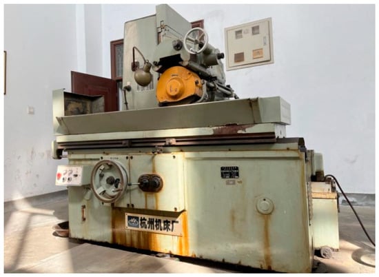
Figure 9.
A conventional surface grinder (Model M7150H).
Table 2.
Processing conditions.
The evaluation parameter for surface roughness is the arithmetic mean deviation Ra. The roughness of each sample block surface was measured at six positions, as shown in Figure 10a, using the roughness meter TA260 (Figure 10b). Measurements were performed with a sampling length of 10 mm, employing a combination of S and L filters and a stylus with a conical shape and spherical tip, having a tip radius of rtip = 5 μm. The arithmetic mean of the six measurements was taken as the roughness value of the sample block. The measurement results for all sample blocks are summarized in Table 3.

Figure 10.
Measurement details and measuring instrument.
Table 3.
Surface roughness value (Unit: um).
According to the standards of the International Organization for Standardization (ISO 21920-1:2021) [33], the grinding workpieces were classified into four roughness grades based on the ranges [0.4, 0.8) μm, [0.8, 1.2) μm, [1.2, 1.6) μm, and [1.6, 2.3) μm. Due to factors such as machine tool vibration and abrasive wear of the grinding wheel during actual processing, the number of samples in each roughness grade, prepared according to the designed processing parameters, is uneven.
3.2. Image Acquisition System
The image acquisition system is shown in Figure 11, where (a) depicts the physical setup and (b) shows a schematic diagram. During image acquisition, the grinding sample block is positioned directly beneath the optical axis of the CCD camera. Two strip light sources, aligned parallel to the grinding texture direction of the sample block, illuminate the surface at an appropriate angle. The sample block is placed on an angle gauge to adjust the normal angle between the camera’s optical axis and the measurement surface, as well as the working distance h between the camera optical axis and the workpiece surface, in order to achieve different acquisition conditions. The light intensity is adjusted using the light source controller.
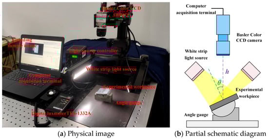
Figure 11.
Image acquisition system.
In order to improve the robustness of the model, multiple conditions are set to add noise to the dataset and increase the number of samples in the dataset, so that the model has stronger recognition ability for grinding surface images collected in variable environments. The parameters of the image acquisition related system are shown in Table 4. During the acquisition process, condition combinations are set for angle , light intensity, and the working distance from the lens to the grinding surface. Figure 12 shows the grinding surface images collected under different environmental conditions. 41 sample blocks were combined with 36 acquisition conditions, resulting in a total of 1476 images collected.
Table 4.
Image acquisition related system parameters.

Figure 12.
Grinding surface images under different environmental conditions (Image size: 640 × 640 pixels).
3.3. Data Partitioning
After setting 36 environmental conditions for each sample block during collection, the acquired images were cropped, resulting in 72 images per sample block. The number of training and testing images after dataset partitioning is shown in Table 5. The test set consists of 144 images, corresponding to two randomly selected samples from each roughness grade, totaling 576 images.
Table 5.
Cropped dataset.
4. Analysis and Discussion of Experimental Results
4.1. Ablation Experiment
This study validated the effectiveness of the added feature extractor through ablation experiments and assessed the impact of removing the deep network structure, as well as the effect of introducing different attention mechanisms on model performance. The validation results are presented in Table 6. Model_a incorporates a feature extractor based on MobileNetV3; Model_b further replaces the original SE attention mechanism in Model_a with the ECA attention mechanism; Model_c is obtained by removing the deep network structure from Model_a.
Table 6.
Ablation results.
According to Table 6, the accuracy of Model_a improved by 0.87% compared to MobileNetV3. This improvement is attributed to the introduction of the feature extractor, which enhances the model’s ability to represent low-level features. Unlike extracting image features from a single perspective, the feature extractor enables the model to capture richer fine-grained information from multiple perspectives. Compared to Model_a, Model_b achieves a 1.04% increase in accuracy while reducing the parameter count by 1.27 M. This is because the ECA attention mechanism avoids the loss of grinding surface information caused by dimensionality reduction in the SE mechanism, and its simpler module structure allows for improved performance with fewer parameters. Model_c, obtained by removing the deep convolutional layers from Model_a, reduces the number of parameters by 3.04 M, yet its accuracy decreases by only 0.87%. This suggests that deep convolutional layers may not be critical for extracting high-level semantic information when identifying surface roughness in grinding. Finally, GE-MobileNet improves accuracy by 2.26% compared to Model_c, further demonstrating the superiority of the ECA attention mechanism over the SE attention mechanism.
4.2. Model Comparison Analysis
To evaluate the overall performance of GE-MobileNet, this study selected MobileNetV3, GhostNetV2, and MobileViTv3 as comparative models for this experiment. MobileNetV3 and GhostNetV2 are widely used and well-established lightweight convolutional networks, while MobileViTv3 represents a state-of-the-art lightweight network that combines Transformer and CNN architectures.
The results of the model comparison experiment are shown in Table 7. It can be seen that GE-MobileNet achieves the highest accuracy, precision, and F1 score. Its accuracy reached 94.97%, which is 2.26%, 7.99%, and 11.29% higher than MobileNetV3, GhostNetV2, and MobileViTv3, respectively. The precision reached 94.94%, representing increases of 1.57%, 7.4%, and 10.68%, respectively, while the F1 score reached 94.95%, surpassing the other models by 1.91%, 7.69%, and 10.98%, respectively.
Table 7.
Performance comparison of each network model on the test set.
As shown in Table 7, GE-MobileNet achieves both the highest mean values and the lowest variances for all metrics, indicating superior stability and robustness across repeated experiments. Moreover, its parameter count remains at the same order of magnitude as the other networks, demonstrating a favorable balance between model complexity and performance.
Overall, these experimental results demonstrate that GE-MobileNet provides not only higher classification accuracy but also more consistent and reliable performance on the test set compared with the other lightweight models.
Figure 13 shows the accuracy–loss (Acc–Loss) curves of each model in the comparative experiment. As shown in Figure 13a, the loss curve of GE-MobileNet converges faster than those of the other models within the first 50 epochs and exhibits relatively small oscillations. In contrast, the loss curve of MobileNetV3 shows more pronounced oscillations between 25 and 100 epochs, while GhostNetV2 and MobileViTv3 continue to exhibit larger oscillations even after 100 epochs. This indicates that GE-MobileNet demonstrates superior stability and learning representation capability compared to the other models. Figure 13b shows that after 150 epochs, GE-MobileNet achieves the highest average accuracy. These experimental results indicate that the newly designed lightweight network GE-MobileNet possesses stronger feature extraction capabilities and outperforms other mainstream models in the task of grinding surface roughness detection.

Figure 13.
Acc–Loss curves of each model in comparative experiment.
The confusion matrices of each model on the test set are shown in Figure 14. GE-MobileNet achieves an accuracy of 99.31% for the first category, which is 9.73%, 6.25%, and 19.45% higher than MobileNetV3, GhostNetV2, and MobileViTv3, respectively. For the second category, GE-MobileNet also achieves 99.31% accuracy, surpassing the other three models by 2.09%, 15.28%, and 21.53%, respectively. The high classification performance of GE-MobileNet in the first two categories demonstrates its excellent feature extraction capability for grinding surfaces with unclear texture information. However, the accuracy for the third and fourth categories is only 90.28% and 90.97%, respectively, which is attributed to the relatively small number of samples in these categories, limiting the model’s ability to fully learn their features. Overall, GE-MobileNet outperforms the other three models across all roughness grades, making it particularly suitable for applications in grinding surface roughness measurement tasks.
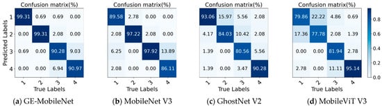
Figure 14.
Cconfusion matrix of each model on the test set.
4.3. Discussion
In actual online measurement scenarios, the camera is generally fixed, resulting in constant imaging distance and angle; however, the on-site lighting environment is often difficult to control [34]. Visual measurement is typically sensitive to lighting conditions, and variations in illumination intensity can affect the model’s performance in image classification [21]. In the previous experiments, the lighting conditions for samples in the training and testing sets were consistent. Although the light intensity during image acquisition varied, the model’s robustness to different lighting conditions could not be fully verified.
To investigate the light source robustness of the GE-MobileNet model, this study retained only images collected under 400–900 LUX and 1200–1700 LUX in the training set, reducing the number of training samples to two-thirds of the original, totaling 1584 images. In the test set, only images collected under 1900–2300 LUX were retained, resulting in one-third of the original samples, totaling 192 images. The experimental hyperparameters were kept consistent with the previous experiment, with the number of epochs set to 200. The experimental results are presented in Figure 15.
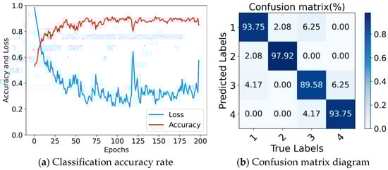
Figure 15.
Effect of GE-MobileNet on grinding images under unknown light source environment.
After 200 epochs, the model achieved a maximum accuracy of 93.75%. These results indicate that the model maintains high recognition accuracy for grinding images under 1900–2300 LUX illumination, even without prior exposure during training. As shown in Figure 15a, the overall loss exhibits a converging trend, but with significant oscillations. This is attributed to the small number of samples in the light source robustness experiment and the substantial distribution differences between the unseen lighting images and the training set, which prevent the loss curve from converging smoothly during training. Figure 15b shows that GE-MobileNet achieves recognition accuracies of 93.75% and 97.92% for the first and second categories of grinding images under unknown lighting conditions, respectively. This demonstrates that the model retains strong capability in extracting fine features of the grinding surface even under varying illumination, confirming its robustness to lighting conditions.
To further improve the training process and accuracy, a larger dataset is required, especially for grinding samples with random surface textures. More data will allow the model to fully learn the subtle features of the grinding surfaces, thereby enhancing its generalization ability. In future work, this study aims to build more comprehensive datasets to ensure that the sample data meets practical industrial standards. Additionally, this study plans to deploy the model on various embedded hardware platforms to construct an online recognition and measurement system for grinding surface roughness.
5. Conclusions
This study proposes a novel GE-MobileNet network for detecting grinding surface roughness, effectively addressing the challenges of roughness classification caused by random surface textures and difficult feature extraction. Ablation experiments verified that the introduction of the GhostNetV2 feature extractor and the ECA attention mechanism improved model accuracy by 2.26%, while keeping the model lightweight with only 5.72 M parameters. A comprehensive performance comparison with mainstream lightweight networks, including MobileNetV3, GhostNetV2, and MobileViT V3, demonstrated that GE-MobileNet achieves superior performance, attaining the highest accuracy, precision, and F1-score, reaching 94.97%. As shown in Table 7, GE-MobileNet also exhibits the lowest variance across repeated experiments, indicating strong stability and robustness. Further analysis under varying lighting conditions showed that the model maintains a recognition accuracy of 93.75%, highlighting its robustness to illumination changes.
The proposed GE-MobileNet combines high accuracy, robustness, and a lightweight design, making it suitable for real-time and embedded applications. The method is practical and cost-effective, as it can be implemented on standard industrial cameras and low-cost embedded devices, such as a Raspberry Pi, providing a user-friendly environment for practitioners. However, the model was trained and tested on a relatively small dataset of grinding surfaces, which may limit its generalization to more diverse industrial conditions. Future work will focus on expanding the dataset, enhancing the network to handle more complex surface textures, and integrating the model into online grinding process monitoring systems. Overall, GE-MobileNet provides a solid foundation for accurate and efficient online measurement of grinding surface roughness using lightweight networks.
5.1. Disclosures
The authors declare that they have no known competing financial interests or personal relationships that could have appeared to influence the work reported in this paper.
5.2. Materials Availability
The data that support the findings of this study are available on request from the corresponding author. The data are not publicly available due to privacy or ethical restrictions.
Author Contributions
Methodology, H.W.; Writing—original draft, F.S.; Writing—review & editing, H.Y. All authors have read and agreed to the published version of the manuscript.
Funding
This work was supported by the National Natural Science Foundation of China (NSFC) under Grant No. 52065016. The APC was funded by the same grant.
Institutional Review Board Statement
Not applicable.
Informed Consent Statement
Not applicable.
Data Availability Statement
The raw data supporting the conclusions of this article will be made available by the authors on request.
Conflicts of Interest
The authors declare no conflict of interest.
References
- Karkalos, N.E.; Galanis, N.I.; Markopoulos, A.P. Surface roughness prediction for the milling of Ti–6Al–4V ELI alloy with the use of statistical and soft computing techniques. Measurement 2016, 90, 25–35. [Google Scholar] [CrossRef]
- Zhang, S.J.; To, S.; Wang, S.J.; Zhu, Z.W. A review of surface roughness generation in ultra-precision machining. Int. J. Mach. Tools Manuf. 2015, 91, 76–95. [Google Scholar] [CrossRef]
- Persson, B.N.J. On the use of surface roughness parameters. Tribol. Lett. 2023, 71, 29. [Google Scholar] [CrossRef]
- Whitehouse, D.J. Handbook of Surface and Nanometrology; Taylor & Francis: New York, NY, USA, 2002. [Google Scholar]
- Gadelmawlaa, E.S.; Kourab, M.M.; Maksoudc, T.M.A.; Elewaa, I.M.; Soliman, H.H. Roughness parameters. J. Mater. Process. Technol. 2002, 123, 133–145. [Google Scholar] [CrossRef]
- Shahabi, H.H.; Ratnam, M.M. Noncontact roughness measurement of turned parts using machine vision. Int. J. Adv. Manuf. Technol. 2010, 46, 275–284. [Google Scholar] [CrossRef]
- Ghodrati, S.; Kandi, S.G.; Mohseni, M. Nondestructive, fast, and cost-effective image processing method for roughness measurement of randomly rough metallic surfaces. J. Opt. Soc. Am. A 2018, 35, 998–1013. [Google Scholar] [CrossRef]
- Pavliček, P.; Mikeska, E. White-light interferometer without mechanical scanning. Opt. Lasers Eng. 2020, 124, 105800. [Google Scholar] [CrossRef]
- Wang, H.; Wei, C.; Tian, A.; Liu, B.; Zhu, X. Surface roughness detection method of optical elements based on region scattering. In Proceedings of the 10th International Symposium on Advanced Optical Manufacturing and Testing Technologies: Advanced and Extreme Micro-Nano Manufacturing Technologies, Chengdu, China, 14–17 June 2021; Volume 12073, pp. 174–181. [Google Scholar]
- Huang, P.B.; Inderawati, M.M.W.; Rohmat, R.; Sukwadi, R. The development of an ANN surface roughness prediction system of multiple materials in CNC turning. Int. J. Adv. Manuf. Technol. 2023, 125, 1193–1211. [Google Scholar] [CrossRef]
- Huaian, Y.I.; Jian, L.I.U.; Enhui, L.U.; Peng, A.O. Measuring grinding surface roughness based on the sharpness evaluation of colour images. Meas. Sci. Technol. 2016, 27, 025404. [Google Scholar] [CrossRef]
- Huaian, Y.; Xinjia, Z.; Le, T.; Yonglun, C.; Jie, Y. Measuring grinding surface roughness based on singular value entropy of quaternion. Meas. Sci. Technol. 2020, 31, 115006. [Google Scholar] [CrossRef]
- Wang, Y.H.; Lai, J.Y.; Lo, Y.C.; Shih, C.H.; Lin, P.C. An Image-Based Data-Driven Model for Texture Inspection of Ground Workpieces. Sensors 2022, 22, 5192. [Google Scholar] [CrossRef]
- ELGhadoui, M.; Mouchtachi, A.; Majdoul, R. Intelligent surface roughness measurement using deep learning and computer vision: A promising approach for manufacturing quality control. Int. J. Adv. Manuf. Technol. 2023, 129, 3261–3268. [Google Scholar] [CrossRef]
- Shi, Y.; Li, B.; Li, L.; Liu, T.; Du, X.; Wei, X. Automatic non-contact grinding surface roughness measurement based on multi-focused sequence images and CNN. Meas. Sci. Technol. 2023, 35, 035029. [Google Scholar] [CrossRef]
- Huang, J.; Yi, H.; Fang, R.; Song, K. A grinding surface roughness class recognition combining red and green information. Metrol. Meas. Syst. 2023, 30, 689–702. [Google Scholar] [CrossRef]
- Howard, A.; Sandler, M.; Chu, G.; Chen, L.C.; Chen, B.; Tan, M.; Wang, W.; Zhu, Y.; Pang, R.; Vasudevan, V.; et al. Searching for MobileNetv3. In Proceedings of the IEEE/CVF International Conference on Computer Vision, Seoul, Republic of Korea, 27 October–2 November 2019; pp. 1314–1324. [Google Scholar]
- Tang, Y.; Han, K.; Guo, J.; Xu, C.; Xu, C.; Wang, Y. GhostNetv2: Enhance cheap operation with long-range attention. Adv. Neural Inf. Process. Syst. 2022, 35, 9969–9982. [Google Scholar]
- Wadekar, S.N.; Chaurasia, A. Mobilevitv3: Mobile-friendly vision transformer with simple and effective fusion of local, global and input features. arXiv 2022, arXiv:2209.15159. [Google Scholar]
- Chen, Y.; Dai, X.; Chen, D.; Liu, M.; Dong, X.; Yuan, L.; Liu, Z. Mobile-former: Bridging MobileNet and transformer. In Proceedings of the IEEE/CVF Conference on Computer Vision and Pattern Recognition, New Orleans, LA, USA, 19–24 June 2022; pp. 5270–5279. [Google Scholar]
- Yi, H.; Wang, H.; Shu, A.; Huang, J. Changeable environment visual detection of grinding surface roughness based on lightweight network. Nondestruct. Test. Eval. 2024, 40, 1117–1140. [Google Scholar] [CrossRef]
- Wei, X.S.; Song, Y.Z.; Mac Aodha, O.; Wu, J.; Peng, Y.; Tang, J.; Yang, J.; Belongie, S. Fine-grained image analysis with deep learning: A survey. IEEE Trans. Pattern Anal. Mach. Intell. 2021, 44, 8927–8948. [Google Scholar] [CrossRef]
- Zhao, B.; Feng, J.; Wu, X.; Yan, S. A survey on deep learning-based fine-grained object classification and semantic segmentation. Int. J. Autom. Comput. 2017, 14, 119–135. [Google Scholar] [CrossRef]
- Zhao, Y.; Yan, K.; Huang, F.; Li, J. Graph-based high-order relation discovery for fine-grained recognition. In Proceedings of the IEEE/CVF Conference on Computer Vision and Pattern Recognition, Virtual, 19–25 June 2021; pp. 15079–15088. [Google Scholar]
- Lin, T.Y.; RoyChowdhury, A.; Maji, S. Bilinear CNN models for fine-grained visual recognition. In Proceedings of the IEEE International Conference on Computer Vision, Santiago, Chile, 7–13 December 2015; pp. 1449–1457. [Google Scholar]
- Song, J.; Yang, R. Feature boosting, suppression, and diversification for fine-grained visual classification. In Proceedings of the 2021 International Joint Conference on Neural Networks (IJCNN), Virtual, 18–22 July 2021; pp. 1–8. [Google Scholar]
- Huang, J.; Yi, H.; Shu, A.; Tang, L.; Song, K. Visual measurement of grinding surface roughness based on feature fusion. Meas. Sci. Technol. 2023, 34, 105019. [Google Scholar] [CrossRef]
- Tan, M.; Chen, B.; Pang, R.; Vasudevan, V.; Sandler, M.; Howard, A.; Le, Q.V. Mnasnet: Platform-aware neural architecture search for mobile. In Proceedings of the IEEE/CVF Conference on Computer Vision and Pattern Recognition, Long Beach, CA, USA, 15–21 June 2019; pp. 2820–2828. [Google Scholar]
- Yang, T.J.; Howard, A.; Chen, B.; Zhang, X.; Go, A.; Sandler, M.; Sze, V.; Adam, H. Netadapt: Platform-aware neural network adaptation for mobile applications. In Proceedings of the European Conference on Computer Vision (ECCV), Munich, Germany, 8–14 September 2018; pp. 285–300. [Google Scholar]
- Hu, J.; Shen, L.; Sun, G. Squeeze-and-excitation networks. In Proceedings of the IEEE Conference on Computer Vision and Pattern Recognition, Salt Lake City, UT, USA, 18–22 June 2018; pp. 7132–7141. [Google Scholar]
- Han, K.; Wang, Y.; Tian, Q.; Guo, J.; Xu, C.; Xu, C. Ghostnet: More features from cheap operations. In Proceedings of the IEEE/CVF Conference on Computer Vision and Pattern Recognition, Virtual, 13–19 June 2020; pp. 1580–1589. [Google Scholar]
- Wang, Q.; Wu, B.; Zhu, P.; Li, P.; Zuo, W.; Hu, Q. ECA-Net: Efficient channel attention for deep convolutional neural networks. In Proceedings of the IEEE/CVF Conference on Computer Vision and Pattern Recognition, Virtual, 13–19 June 2020; pp. 11534–11542. [Google Scholar]
- ISO 21920-1:2021; Geometrical Product Specifications (GPS)—Surface Texture: Profile—Part 1: Indication of Surface Texture. International Organization for Standardization: Geneva, Switzerland, 2021. Available online: https://www.iso.org/standard/72276.html (accessed on 1 January 2024).
- Hutchings, A.; Hollywood, J.; Lamping, D.L.; Pease, C.T.; Chakravarty, K.; Silverman, B.; Choy, E.H.S.; Scott, D.G.; Hazleman, B.L.; Bourke, B.; et al. Roughness classification detection of Swin Transformer model based on the multi-angle and convertible image environment. Nondestruct. Test. Eval. 2023, 38, 394–411. [Google Scholar] [CrossRef]


Disclaimer/Publisher’s Note: The statements, opinions and data contained in all publications are solely those of the individual author(s) and contributor(s) and not of MDPI and/or the editor(s). MDPI and/or the editor(s) disclaim responsibility for any injury to people or property resulting from any ideas, methods, instructions or products referred to in the content. |
© 2025 by the authors. Licensee MDPI, Basel, Switzerland. This article is an open access article distributed under the terms and conditions of the Creative Commons Attribution (CC BY) license (https://creativecommons.org/licenses/by/4.0/).