Article

Engineering-Scale B-Spline Surface Reconstruction Using a Hungry Predation Algorithm, with Validation on Ship Hulls

Department of Mechanical Engineering, Dalian Maritime University, Dalian 116026, China
*
Author to whom correspondence should be addressed.
Appl. Sci. 2025, 15(21), 11471; https://doi.org/10.3390/app152111471
Submission received: 10 September 2025 / Revised: 16 October 2025 / Accepted: 23 October 2025 / Published: 27 October 2025
(This article belongs to the Section Mechanical Engineering)

Abstract

This paper tackles a core challenge in reverse engineering: high-fidelity reconstruction of continuous B-spline surfaces from discrete point clouds, where optimal knot placement remains pivotal yet not fully resolved. We propose a new fitting method based on the Hungry Predation Algorithm (HPA) to improve efficiency, accuracy, and robustness. This method introduces a hybrid knot-guidance strategy that combines geometry-aware preselection with a complexity-driven probabilistic distribution to address knot placement. On the optimization side, HPA simulates starvation-driven predator–prey dynamics to enhance global search capability, maintain population diversity, and accelerate convergence. We also develop an adaptive parameter adjustment framework that automatically tunes key settings according to surface complexity and accuracy thresholds. Comparative experiments against classical approaches, six state-of-the-art optimizers, and the commercial CAD system CATIA demonstrate HPA’s superiority in control-point reduction, fitting accuracy, and computational efficiency. This method shows high applicability to engineering-scale tasks (e.g., ship hull design), where the point-to-surface RMSE (e.g., <10−3 Lmax) achieved satisfies stringent requirements for downstream hydrodynamic performance analysis and manufacturing.

1. Introduction

The purpose of this paper is to investigate B-spline surface fitting for industrial products, which falls under the broader category of surface reconstruction in reverse engineering [1,2]. In reverse engineering, laser scanning or other acquisition techniques are employed to obtain point cloud data containing geometric information of the product. However, the point cloud is a discrete data structure that lacks topological information. To effectively support downstream tasks such as geometric feature modification and multidisciplinary simulations, it is necessary to convert the point cloud into a continuous geometric model with embedded topological information [3]. B-splines possess several desirable properties, including locality, parametric continuity, and geometric invariance. As a result, they are recognized by the International Organization for Standardization (ISO) as a standard method for describing product geometry [4] and have become an important interface between reverse engineering and other engineering disciplines [5,6,7,8]. Converting discrete point clouds into continuous B-spline surfaces is a critical enabling technology for model integration and remains a research hotspot in the field of B-spline surface modeling.
Surface reconstruction generally involves two approaches: interpolation and approximation. In the B-spline interpolation method, the number of control points is determined by both the degree of the surface and the number of data points. The interpolation surface generally suffers from poor smoothness. Moreover, when handling large-scale point cloud data, it often results in an excessive number of control points, making efficient data exchange difficult to achieve. Compared with interpolation, B-spline surface approximation offers greater flexibility in representing and designing surface shapes. However, the number of control points required to achieve a given approximation accuracy is typically unknown beforehand. The essential problem is the knot placement. Existing methods can be categorized into static and dynamic knot strategies, depending on whether the knot positions are adjusted after initial placement. Unreasonable knot placement may lead to unacceptable shapes. Currently, researchers consider fitting accuracy [9,10], the number of knots [1,3], and computational efficiency [11,12] as key performance metrics for evaluating approximation methods.
Building upon previous work on B-spline curve fitting [13], this paper develops a B-spline surface fitting method for industrial products based on the Hungry Predation Algorithm (HPA), aiming to address three key challenges: (1) optimal knot placement [1]; (2) accuracy and convergence of the optimization algorithm [14]; and (3) robustness for practical engineering applications [15]. To address challenges (1) and (2), HPA employs a two-part strategy comprising knot guidance and population-based optimization. The knot guidance strategy places additional knots near complex regions of the model based on point cloud characteristics, thereby enhancing the capture of detail and avoiding poor knot configurations that may arise from random initialization. HPA incorporates neighborhood influence into individual position updates, which helps maintain population diversity and prevents premature convergence due to overcrowding of individuals. In addition, it allows the “hungry” individuals—those with lower fitness—to move rapidly toward the optimal solution, leading to faster convergence of the algorithm. To address this challenge (3), an adaptive parameter tuning method is introduced, which automatically adapts to both the fitting model and the desired accuracy.
The rest of this paper is organized as follows. Section 2 introduces the B-spline surface theory underlying HPA, along with related work on surface reconstruction and B-spline surface fitting. Section 3 presents the HPA method in detail, including a novel knot guidance strategy and the optimization mechanism of the Hungry Predation Algorithm. Section 4 analyzes the key input parameters of HPA, including surface degree, number of knots in the U and V directions, the population mutation rate, population size, and iteration count. Section 5 evaluates the performance of HPA. Compared with a typical static-knot method, a dynamic-knot method, and commercial engineering software, HPA demonstrates superior performance in terms of fitting accuracy and convergence speed. Finally, this paper concludes with a summary of findings and outlines potential directions for future research.

2. Related Theories and Research

2.1. B-Spline Surface Fitting

The B-spline surface fitting problem can be transformed into a series of B-spline curve fitting problems in the U and V directions using the tensor product surface method [4]. Although the processing methods for the U and V directions are similar, they differ in their inputs and outputs. The U-direction takes the original point cloud data as input and produces intermediate control points, while the V-direction uses these intermediate control points as input to generate the final control points.
The knot vector U consists of a non-decreasing sequence u0 ≤ u1 ≤ um+ρ+1, and similarly, the knot vector V is composed of v0 ≤ v1 ≤ vn+ρ+1. Accordingly, there will be a total of (m + 1) × (n + 1) control points di,j, where i = 0, 1, …, m and j = 0, 1, …, n.
Taking the U-direction as an example, the i-th B-spline basis function Ni,ρ(u) of degree ρ (order ρ + 1), is defined using the Cox–de Boor recursion formula, as shown in Equation (1).
N i , 0 u = 1                   u i     u       u i + 1       ( i   =   0 ,   ,   m )
0     other
N i , ρ ( u ) = u u i u i + ρ u i N i , ρ 1 ( u ) + u i + ρ + 1 u u i + ρ + 1   u i + 1 N i + 1 , ρ 1 ( u )  
The standard cumulative chord length method is adopted to parameterize the data point cloud. For each direction, the arithmetic mean of the parameterization results from all curves is used to obtain the final parameter values. To compute the control points of the B-spline surface, a standard least-squares minimization method is employed, along with endpoint constraints to ensure geometric continuity.
After processing both the U and V directions, the B-spline surface is fitted using the computed control points and corresponding B-spline basis functions, as defined in Equation (2).
  p ( u ,   v ) = i = 0 m j = 0 n d i , j N i , k ( u ) N j , l ( v )     u ,   v     [ 0 ,   1 ]      
where Ni,k(u) and Nj,l(v) are B-spline basis functions in the U and V directions, respectively.
Fitness   1   = Max ( Q i r Q i f )  
Fitness   2 = i = 1 N p | Q i r Q i f | N p      
Fitness   3 = i = 1 N p | Q i r Q i f | 2 N p          
where Np is the number of data points, and Qir and Qif denote the original data point and the corresponding point on the fitted surface, respectively.
Fitness 1 penalizes the maximum point-wise deviation, while Fitness 2 and Fitness 3 evaluate the overall fitting error across all data points. In particular, the root mean square error is more sensitive to large deviations and is widely adopted in engineering applications. The fitness functions can be used individually or in combination. Unless otherwise specified, the root mean square error is used as the default fitness function in this study.
We prioritize cubic (degree-3) B-splines because they offer a strong balance of smoothness and locality. To maintain generality, both the spline degree and the fitness can be adapted to task requirements. For example, quadratic (C1) with repeated knots for sharp features, or quartic/quintic for ultra-smooth fairness; likewise, the fitness can incorporate curvature-weighted RMSE or stricter maximum-error thresholds when mandated by specific products.

2.2. Research Status

Common surface reconstruction methods in reverse engineering include spline interpolation [16], least-squares approximation [17], and partial differential equation-based methods [18]. Among these methods, spline theory has received considerable attention 1from researchers. Extensive studies have focused on various types of spline functions, such as Hermite splines [19], Bézier splines [20], and B-splines [21]. In particular, the B-spline function is the most widely adopted basis for surface modeling due to its flexibility and robustness. Existing research on B-spline surface fitting can be broadly categorized into static knot methods and dynamic knot methods, based on the strategy used for knot placement. Static knot methods include the averaging technique [4,22], knot removal [23], and feature point-based methods [24,25]. In these approaches, knot positions are fixed once selected and remain unchanged throughout the fitting process until the required accuracy is achieved. The averaging technique is simple and easy to implement [26,27], making it a popular choice for basic surface fitting tasks. The knots are selected to capture the overall distribution of the data points and to ensure that each knot span contains at least one point. However, this method struggles to accurately preserve small-scale features in the point cloud. The knot removal method initializes the fitting process with as many control points as data points [28]. It then iteratively removes knots while maintaining the approximation within a predefined maximum error threshold. However, the computational cost associated with the knot removal method is often prohibitive, particularly when applied to large and densely distributed noisy datasets. The feature point method identifies geometric features of the original curve by preprocessing the input point cloud [1,29]. This method is capable of preserving fine-grained features in the point cloud. However, it typically requires more knots than other methods to achieve the same level of fitting accuracy. The dynamic knot method integrates B-spline surface fitting with metaheuristic optimization techniques, and its overall performance is highly dependent on the effectiveness of the chosen algorithm. One key advantage of the dynamic knot method is that it avoids relying on predefined relationships between knots and the fitting curve, which are often assumed in static methods. Specifically, it performs iterative forward calculations using multiple sets of randomly initialized knot vectors. Based on the optimization algorithm’s iterative mechanism, the knot vector is dynamically updated through real-time feedback. Both the number and positions of the knots are adjusted to improve the fitting performance. Existing research on B-spline surface fitting has applied a variety of intelligent optimization algorithms, including genetic algorithms (GA) [30], detection-based methods [31], artificial immune systems [32,33], and Pareto envelope-based selection algorithms [34,35,36]. In particular, for complex B-spline surface fitting tasks, dynamic knot methods can significantly reduce the number of required knots. However, these optimization algorithms often require a large population size and a high number of iterations to ensure stability and reliability. As a result, their computational cost is typically much higher than that of static knot methods.

3. B-Spline Surface Fitting Based on HPA

This section describes the application and computational framework of the Hungry Predation Algorithm (HPA) for B-spline surface reverse fitting. Unlike B-spline curve fitting, surface fitting requires the simultaneous optimization of knot vectors and control points in both the u- and v-directions. This increases computational complexity significantly and enlarges the search space of the optimization problem. When dealing with high-dimensional point cloud data or complex freeform surfaces, the absence of an effective initialization strategy can lead to slow convergence or entrapment in local optima. To address this, a geometry-aware and complexity-driven knot guidance strategy is introduced prior to the application of HPA to improve fitting efficiency and convergence rate. This approach adaptively generates initial knot distributions over the parametric domain, serving as a high-quality starting point for subsequent optimization.

3.1. Hybrid Initial Knot Guidance Method Based on Multi-Strategy Integration

In B-spline surface approximation, the quality of the initial knot distribution plays a crucial role in determining the convergence speed and final accuracy of the optimization process. To enhance fitting performance while maintaining the diversity of the initial population, this study proposes a hybrid knot initialization strategy that integrates geometry-aware knot guidance, complexity-driven probabilistic sampling and random generation. The entire population is divided into three groups:
30% adopt geometry-aware knot guidance;
50% follow complexity-driven probabilistic sampling;
50% are initialized through uniform random sampling over the domain [0, 1].

3.1.1. Geometry-Aware Knot Guidance

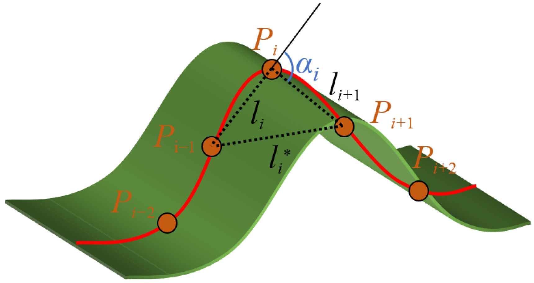
Under the tensor-product paradigm, a surface can be analyzed through a family of iso-parametric (or sectional) curves, which reduces feature detection on the surface for the detection of features on multiple 1D curves. In practical projects, we focus on three types of curve cues that most affect B-spline fitting quality: curvature discontinuities (C1 breaks), curvature extrema (peaks/valleys of |κ|), and inflection points (sign changes of κ), as illustrated in Figure 1.
Let {Pi−1,Pi,Pi+1} be three consecutive samples on a sectional polyline. Define chord lengths
d i 1 = | | P i P i 1 | |         d i = | | P i + 1 P i | |             d i * = | | P i + 1 P i 1 | |      
Let θi be the turning angle between the two consecutive chords, and let Ai denote the oriented area of the triangle (Pi−1,Pi,Pi+1) (positive for counter-clockwise ordering), as shown in Figure 2. We use the following signed curvature indicator, according to Equation (6) [37].
κ u i = 2 A i d i 1 d i d i * = sgn A i sin θ i d i *                                                                                                      
After processing each curve, we obtained the position of the surface feature point [38] and the corresponding parameter values ui and started to select the node vector. Knot guidance means that when the knots are initially selected, they are closer to the complex area of the model. Knots take equal probability values in each interval [ui − 0.1, ui + 0.1]. Each knot has a 50% probability of mutation, and the value interval after mutation is [0, 1]. The knot guidance process in the V direction is similar, but the intermediate control points are used as the data points. In the V-direction, the knot guidance process is based on the intermediate control points, which refer to the control vertices obtained after fitting the surface along the U-direction. These points form a new point cloud in the V-direction and serve as the input for selecting the V-direction knot vector. This two-stage fitting approach ensures that the knot placement in both directions reflects the geometric characteristics of the surface.

3.1.2. Complexity-Driven Probabilistic Guidance

Although the previous section introduced a feature point-based knot guidance strategy using local perturbation intervals, it still has the following limitations:
  • The identification of feature points is discrete in nature and can only guide knot placement around a limited number of critical locations, failing to capture the global geometric complexity of the surface.
  • While local knot densification occurs near feature points, adjacent “semi-complex” regions may still suffer from insufficient knot density, leading to elevated local fitting errors.
To address these issues, this paper further introduces a complexity-driven knot density function as a complement to the existing geometry-aware knot guidance method. The goal is to obtain higher-quality initial knot distributions and enhance the diversity of the optimization algorithm.
(1)
Formulation of the Complexity Function
We define a continuous function D r a w ( u ) over the parametric domain to quantify local complexity by combining two cues, local curvature κ(u) (geometric variation) and point-cloud density ρ(u) (data compactness), as follows Equation (7):
D r a w ( u )   =   ω 1 κ ( u )   +   ω 2 ρ ( u )                   ω 1 , ω 2     0 ,   ω 1   +   ω 2   =   1  
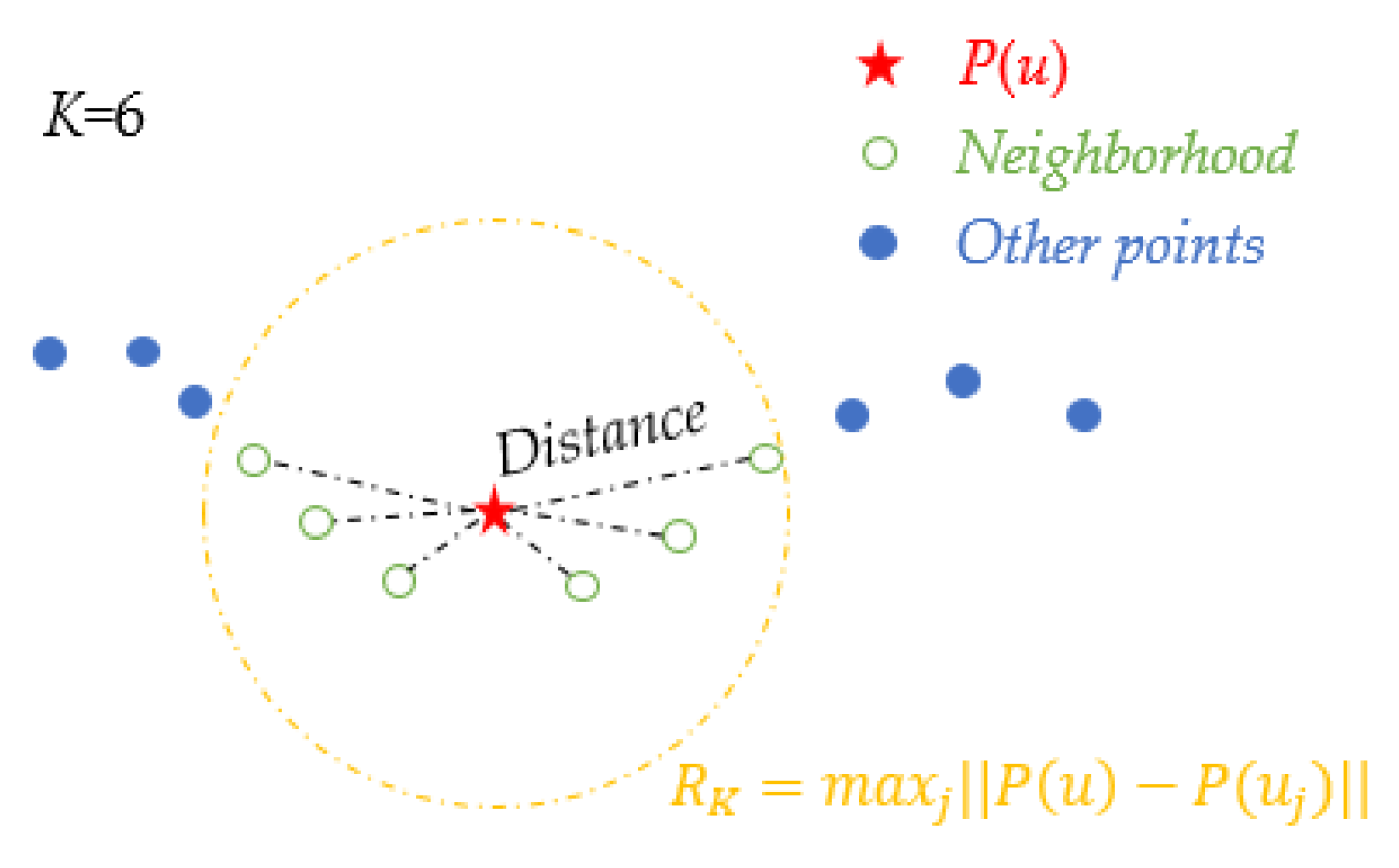
The density cue is defined as the inverse of the mean spacing to the K nearest neighbors { u j } j = 1 K , as shown in Equation (8), and a schematic illustration of this definition is shown in Figure 3.
ρ ( u ) = 1 1 K j = 1 K | | P ( u ) P ( u j ) | |  
where K sets the local scale (typical choices: K = 6–10 for dense/smooth data; K = 3–5 for sparse or sharply varying regions).
Before weighting, each cue is robustly normalized to [0, 1] using 5th–95th percentile scaling, as follows Equation (9):
x ^ u = clip x u P 5 x P 95 x P 5 x , 0 , 1 , x κ , ρ                    
Under this normalization, neither cue has a priori dominance across diverse datasets. We therefore use the reproducible default ω1 = ω2 = 0.5, which follows the principle of indifference, avoids extra hyperparameter search, and prevents over-emphasizing either sharp features or sampling bias. Optionally, (ω1,ω2) can be tuned on a small validation split or made locally adaptive; details are provided in the supplement.
We finally normalize D r a w (u) to obtain a valid probability density for knot sampling, as follows Equation (10):
  D ( u )   =   D r a w ( u ) 0 1 D ( t ) d t           0 1 D ( u ) d u =   1                                                                                            
so that D(u) du gives the probability of placing a knot within [u, u + du], allocating more knots to geometrically complex regions.
(2)
Implementation procedure for knot distribution
To effectively integrate this density function into the population initialization phase, the knot placement process is implemented as follows:
Computation of the Complexity Function
For each fitting curve (or surface profile curve), compute curvature and local point density to construct and normalize the complexity function D(u).
Sampling Knots via Probabilistic Methods
Based on the previously computed D(u), the probability of generating a knot at each data point is proportional to the value of D(u).
Combining with Mutation for Hybrid Distribution
A moderate mutation rate (e.g., 50%) is applied to the complexity-guided knot vectors to avoid overfitting to the initial complexity estimate and to enhance population adaptability.

3.2. Hunger Predation Algorithm Optimization Technology

In HPA, the adaptive adjustment of knots simulates predator–prey behavior under starvation, allowing individuals to rapidly converge toward the current optimal solution. In surface fitting, each individual contains knot vectors in both the U and V directions, and the adaptive adjustment strategy is applied symmetrically to both. The adjustment can be performed sequentially, starting with one direction (e.g., U) followed by the other.
Let W denote the population size and Max_iter the maximum number of iterations. At each iteration, the three individuals with the best fitness are denoted as α, and their knot vectors in the U-direction are recorded as:
Let the population size be W and the maximum number of iterations be Max_iter. At iteration iter, we sort the population by fitness (lower is better) and mark the three best individuals as α1, α2, and α3. Their U-direction knot vectors are
                                                            U p α k = ( u p 1 ,   u p 2 ,   ,   u p D α k )               k   = 1 , 2 , 3  
while a generic (non-elite) individual is denoted as
  U i = ( u i 1 ,   u i 2 ,   ,   u i D )
Elites αk are retained; the remaining individuals (denoted ω) are updated according to Equations (11)–(13).
a = 2 ( iter / Max _ iter )  
U i + 1 α k =   U p α k   A   | C U p α k U i |                       k = 1 ,   2 ,   3  
U i + 1   = k = 1 3 U i + 1 α k / 3  
where A is a random number between [−a, a], and C is a random number between [0, 2].
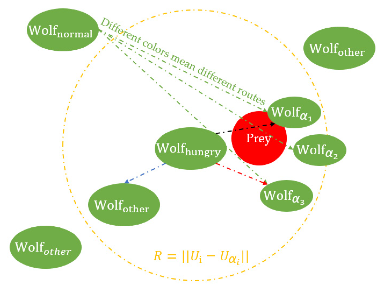
To intensify exploitation around promising regions, each non-elite individual independently becomes “hungry” with probability 0.5. A hungry individual overrides the above step with the following move. First, define a neighborhood radius with respect to the best elite, as shown in Equation (14).
R i = | | U i U α 1 | |  
And the neighbor set is shown in Equation (15).
N i = { U j | D i U i , U j     R i }  
where Di(⋅,⋅) is the distance in the decision space (Euclidean in our implementation). Then choose a reference Ur with probability 0.5 from Uα1, otherwise uniformly from Ni, and perform a cosine–scheduled step, as shown in Equation (16).
U i + 1   =   U r +   U r U i   ×   S   ×   cos ( Iter Max _ iter 0.5 )  
where S is a random number between (0, 1).
After any update, Ui+1 is projected onto the feasible set of nondecreasing knot vectors with boundary clamping (end-conditions), by sorting and min–gap enforcement; an analogous procedure is applied to the V-direction. Elites are copied unchanged to the next generation. Figure 4 sketches the overall HPA search: elites guide conventional updates (Equations (11)–(13)), while probabilistic hungry moves (Equations (14)–(16)) accelerate convergence toward the current prey (best solution) through neighborhood-aware steps and a cosine schedule.

3.3. HPA Process

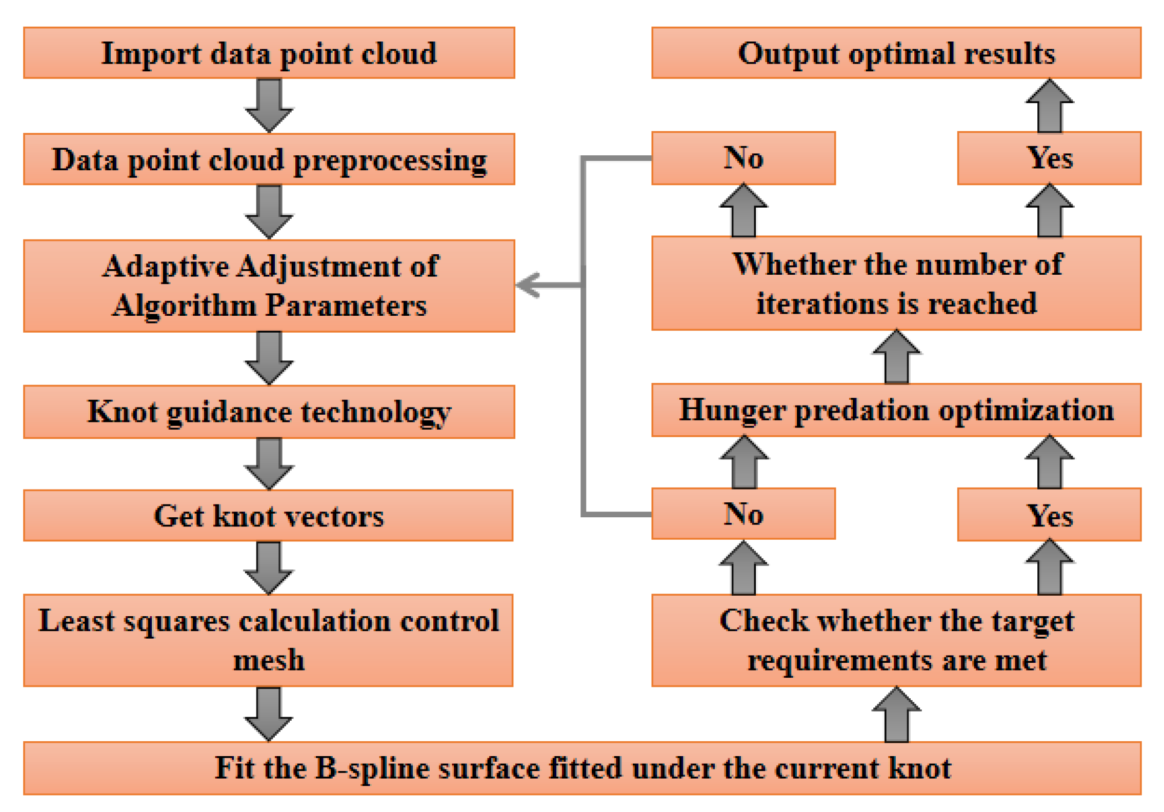
The main flow of HPA is shown in Figure 5.
First, import the data points of the surface, and calculate the curvature of the data points. Then we order the data points and perform the parameterization of the standard accumulation chord length to obtain the corresponding parameter values. The parameters of the algorithm are adaptively adjusted, and the specific content is introduced in Section 4. The U-direction and V-direction knot vectors are obtained through the knot guidance technology; the control point is obtained by the least-squares minimization method, and the B-spline surface under the current knot is obtained. Check whether the current fitting surface meets the requirements. If the dimension of the individual meeting the error threshold is the maximum dimension of the population, or there is no individual meeting the error threshold in the population, the hungry predation algorithm is used for optimization. Otherwise, the parameter setting is returned, the parameters are adjusted adaptively, and the surface fitting is performed again. After completing the hunger predation algorithm, it is judged whether the set iteration number has been reached or the improvement in the best fitness value (e.g., the root mean square error) over consecutive iterations falls below a predefined threshold. The accuracy threshold is set according to enterprise manufacturing tolerances or domain-specific requirements; in our experiments, we adopt 10−3 Lmax unless otherwise stated. If it is reached, the current optimal result will be output. Otherwise, it will return to the algorithm parameter adjustment and continue to find better results.

3.4. Adaptive Adjustment of Input Parameters

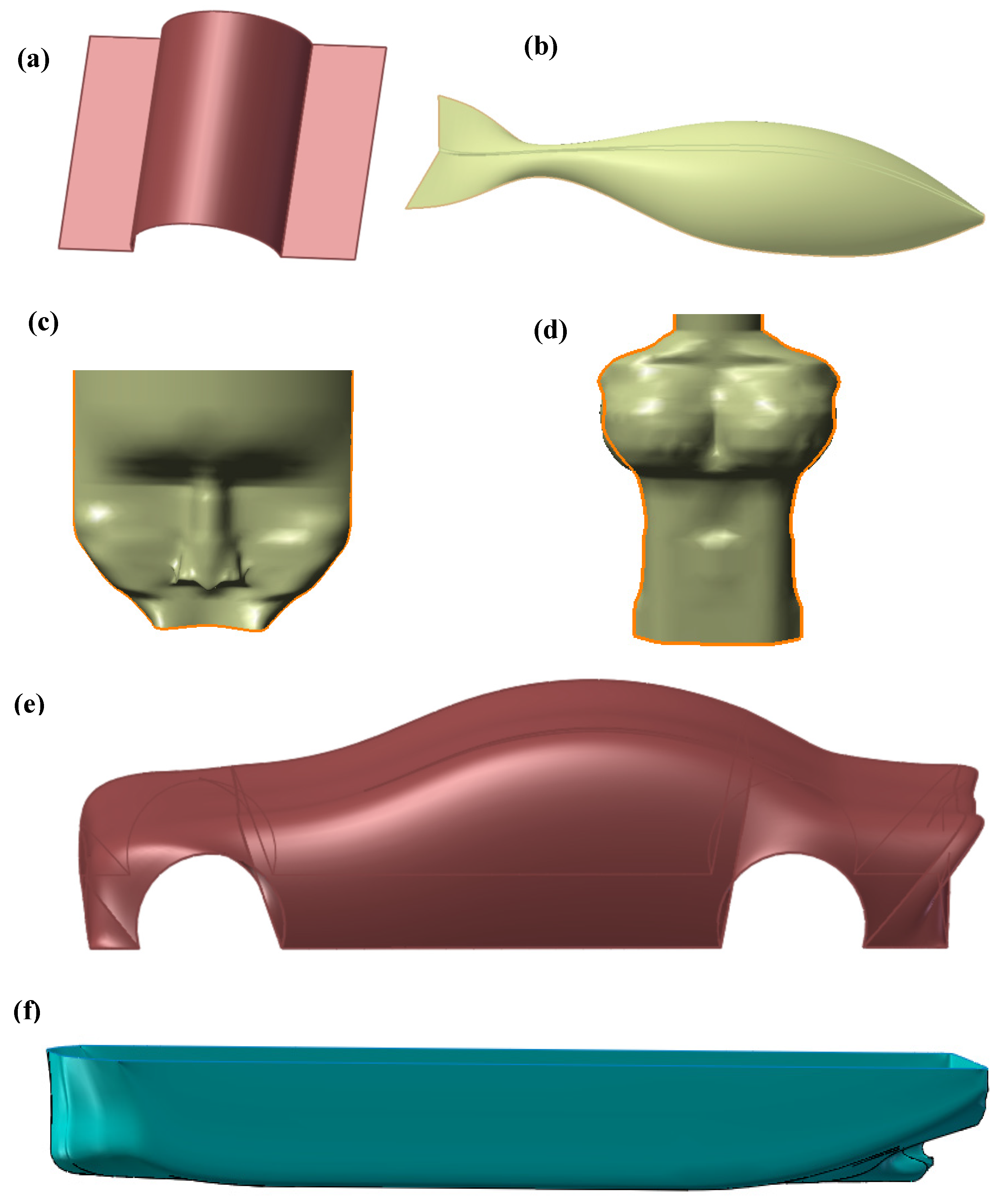
The variables of the algorithm include the degree of the surface, the number of internal knots in the U and V directions, the population mutation rate, the settings of population size W and iteration number Max_iter. The setting method of relevant parameters is obtained by experimental analysis on the elementary analytical surface (Figure 6a), natural free-form surface (Figure 6b–d) and engineering surface (Figure 6e,f) shown in Figure 6.

Internal Knots Number

Each individual in the population has a different dimension or value of initial knots in the initial state, and the internal knot rate determines the range of selecting the number of knots. In the study of curves by Xu S et al., the internal knot rate is uniformly selected as 0–0.5 [38]. When dealing with the surface fitting of a large number of point clouds, if the selection range of the knot number is set too wide, it needs to increase the population size and conduct a large number of iterations to find a satisfactory knot number, which will greatly reduce the computational efficiency of the algorithm. In order to improve the effectiveness of the population, the range of the internal knot rate λ should be narrowed, and a dynamic internal knot rate is proposed for this purpose. The internal knot starts from a higher value first, which is uniformly selected as 0.5–0.8 in this experiment. When the population finds a better solution that uses fewer control points under the premise of satisfying the error threshold, it is necessary to clean up and supplement the existing population. At this time, the range of the internal knot rate λ changes, as shown in Equation (17)
λ u = rand [ N u α p u 0.1 , N u α p u + 0.05 ]  
λ v = rand [ N v α p v 0.1 , N v α p v + 0.05 ]  
where N is the U-direction knot number of the individual Wα1 with the best fitness in the population, N is the V-direction knot number of Wα1, Pu is the data point number in each row of the U-direction, and Pv is the number of intermediate control points in each column in the V-direction.
The above process is repeated until there are no more satisfied solutions with fewer control points in the population. At this time, if the number of individuals meeting the error threshold in the population is less than 4, including 0, the U-direction and V-direction knot vectors of the three individuals with the best fitness are retained. If the number of individuals in the population that meet the error threshold is more than 4, the three individuals with the smallest product of the knot vectors in the U and V directions are retained. Then, other individuals in the population are emptied and the remaining (W-3) individuals are replenished. For most models, HPA can find the knot vector that meets or approaches the given error threshold in the first iteration. The problem is that the control mesh may not be the simplest. For the supplement of the population, the number of U-direction knots Nuω is shown in Equation (18).
N u ω =   rand [ N u α 2 ,   N u α + 1 ]  
The corresponding number of V-direction knots Nvω is shown in Equation (19).
N v ω =   N u α   ×   N v α   N u ω  
where   is the downward rounding symbol.

4. Surface Degree and Population Mutation Rate

The degree of the surface includes the degree of the U-direction and V-direction curves, which are uniformly selected three times. In practical industrial applications, our algorithm should have good universality. For different shape problems, if high-order curves are used to fit, the corresponding appropriate number of times cannot be directly given, so that a large number of calculations and tests are required. An inappropriate degree may lead to results that are difficult to meet the approximation accuracy. The cubic curve is not only a plane curve with an inflection point, but also the lowest degree that can generate a space curve, and can describe a complex shape curve through multiple segments.
In Section 3.1, we introduce the knot guidance technology to realize the distribution of knots at the complex surface in the knot preselection stage. When the knot selection process is completely based on the knot guidance technology, that is, the mutation rate is 0, the diversity of the population is destroyed, and the knots are concentrated near the characteristic points, resulting in a low effective population number. When there is no knot guidance, that is, the mutation rate is 100%, and the knots are randomly distributed. When dealing with complex models with uneven distribution of feature points, it is difficult to obtain an effective initial knot number.
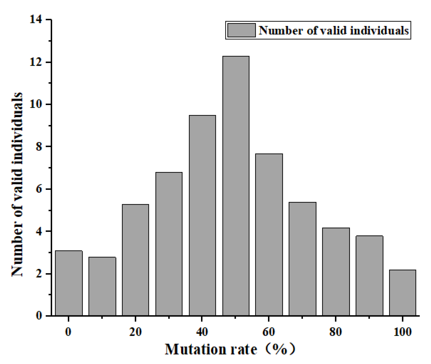
After testing several models, it is found that when the knots are guided and the mutation rate is set to 50%, the initial knots will probably appear at the feature points, and the 50% mutation rate ensures that the population diversity is not destroyed. Taking the population size 20 as an example, the reasonable results number in the model of Figure 6f with or without knot guidance and different mutation rates V when solving the U-direction intermediate control point are compared, as shown in Figure 7.
It can be seen that the effective rate in this population is 6 times higher than that in the case of no knot guidance.

Population Size and Iteration Number

Let W denote the population size (number of concurrent search trajectories) and Max_iter the iteration budget (search depth). Each individual carries its own U- and V-direction knot vectors. Larger W improves breadth/exploration and the chance of locating high-quality solutions, whereas larger Max_iter increases depth/exploitation of promising regions. Both parameters, therefore, jointly control accuracy, robustness, and cost.
We first fix Max_iter ∈ {10, 20} and gradually increase W from 10 to 20; a representative run is shown in Figure 8a. We then evaluate three budget levels (W, Max_iter) ∈ {(10, 10), (20, 20), (30, 30)} and perform 10 independent trials for each setting; aggregated results are summarized in Figure 8b.
It can be seen from the experimental results that when the W and Max_iter are small, the algorithm is less stable and may fail to meet the accuracy threshold in some runs. Increasing either parameter raises the probability of good outcomes, improves stability, and typically yields fewer control points for the same accuracy.
In B-spline surface fitting, the decision variables are ordered knots in [0, 1], and the search difficulty depends on the tolerance, scale, and geometric complexity. To avoid brittle manual tuning, we adopt the following rules, as shown in Equations (20) and (21).
W = In ( E L Max )   ×   1.2 Log 10 ( L Max E ) + 1.5   ×   Cp  
Max _ iter = 2   ×   W    
where L Max is the model’s maximum side length, Cp is the number of feature points on the most complex sectional curve, and “⌊⌋” denotes the floor operation.
With Equations (20) and (21), the user only provides data points and the desired tolerance; W and Max_iter are then adapted automatically, yielding good accuracy–efficiency trade-offs across models.

5. Experimental Comparisons

The experiment is divided into two parts. Section 5.1 is compared with the typical static knot method and dynamic knot method, and Section 5.2 is compared with the existing commercial software CATIA 2022 (Dassault Systèmes SE, Vélizy-Villacoublay, France).

5.1. Comparison with Existing Research

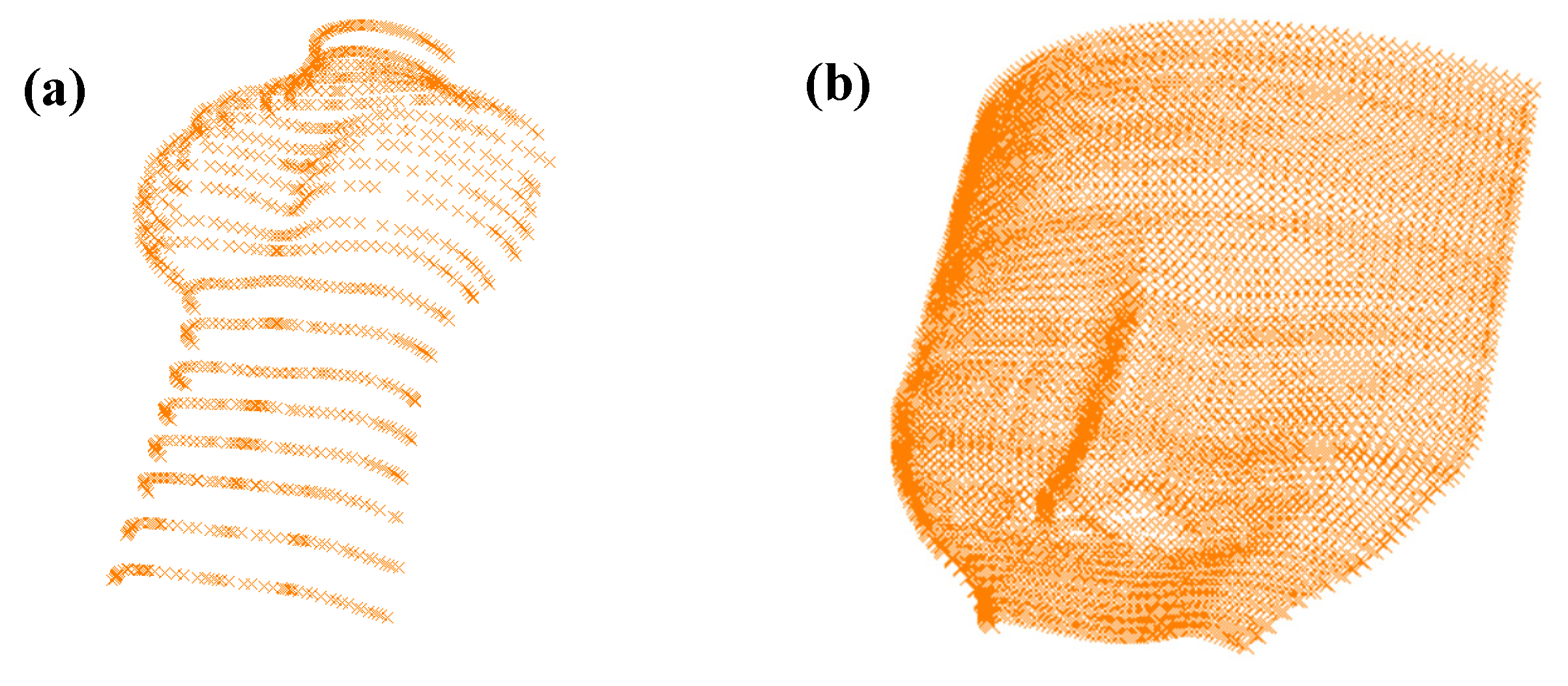
Refs. [1,26] realize the fitting of free-form surfaces. Based on the experiments mentioned in the two papers, the model point cloud is extracted, and the approximate surface is reconstructed, as shown in Figure 9. The control point number used by different algorithms is compared at the same precision.
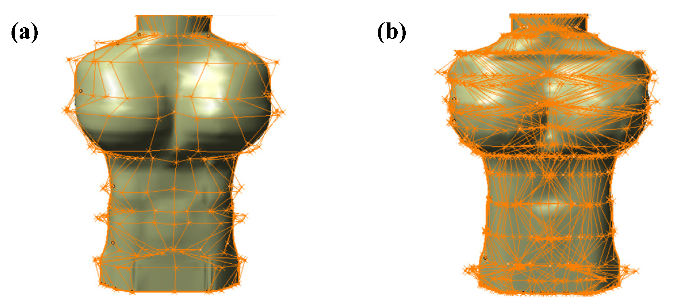
In the study of Figure 9a, innovation lies in the reduction in data points, and the remaining data points are fitted by interpolation. The HPA method is used to fit the human model in this paper, and the fitting is shown in Figure 10.
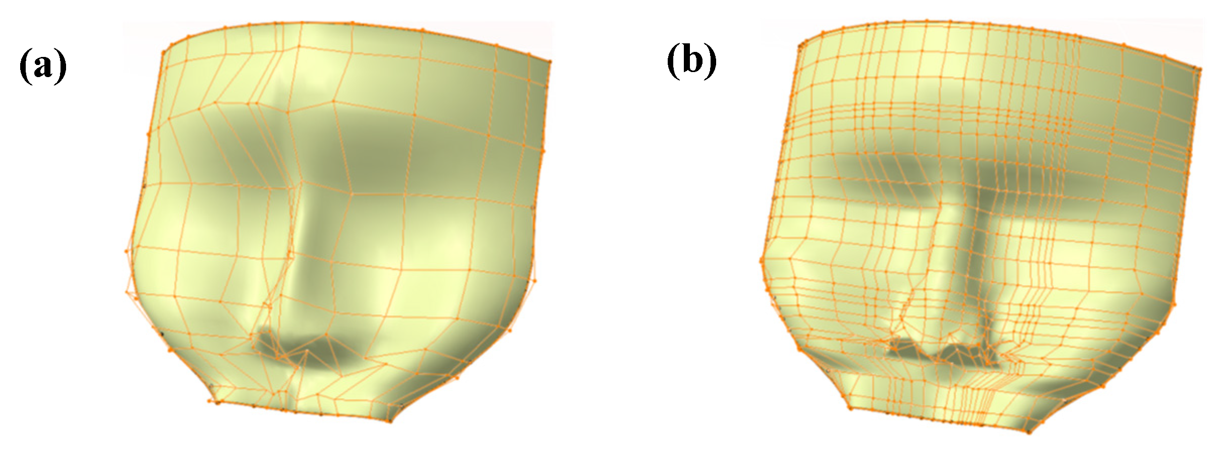
In the study, in Figure 9b, the dominant column of the surface is selected and the knot placement averaging technology method is used. When the error threshold is not met, insert the dominant column repeatedly until the condition is met. The HPA is used to fit the face model in its experiment, and the fitting results are shown in Figure 11.
Compared with related methods, HPA uses fewer control points under the same fitting effect, as shown in Table 1.
The disadvantage of the optimization algorithm is that it takes a lot of attempts to find the optimal solution in a space, which leads to the optimization algorithm method needing more time than other methods. Table 2 records the operation efficiency and fitting accuracy of relevant algorithms in the existing literature.
Running time and efficiency are important factors in evaluating the algorithm. However, due to different research times, there are certain differences in both hardware and software, and there is no unified test model in relevant studies. Different data point clouds and knot numbers will have a great impact on the running time. It is not objective to compare the running time. In order to objectively evaluate the operation efficiency of each algorithm as much as possible, this paper reproduces the six optimization algorithms WOA [43], GSA [44], EA [45], GWO [46], PSO [14] and DE [47]. We selected these six methods because they span the mainstream metaheuristic families for continuous optimization that are most often used in curve/surface fitting: swarm-intelligence (PSO, GWO, WOA), evolutionary heuristics (DE, EA), and physics-inspired search (GSA). They are widely cited, have stable open implementations and low tuning overhead, and exhibit complementary exploration–exploitation behaviors, providing a balanced and representative benchmark panel.
Run them under the condition that W is 30, Max_iter is 50, and the error threshold is one thousandth of the maximum side length of the model. The six models in Figure 6 are fitted to compare the search ability of each algorithm. The specific parameter settings of each algorithm are shown in Table 3, and the results of the primary experiment are shown in Figure 12.
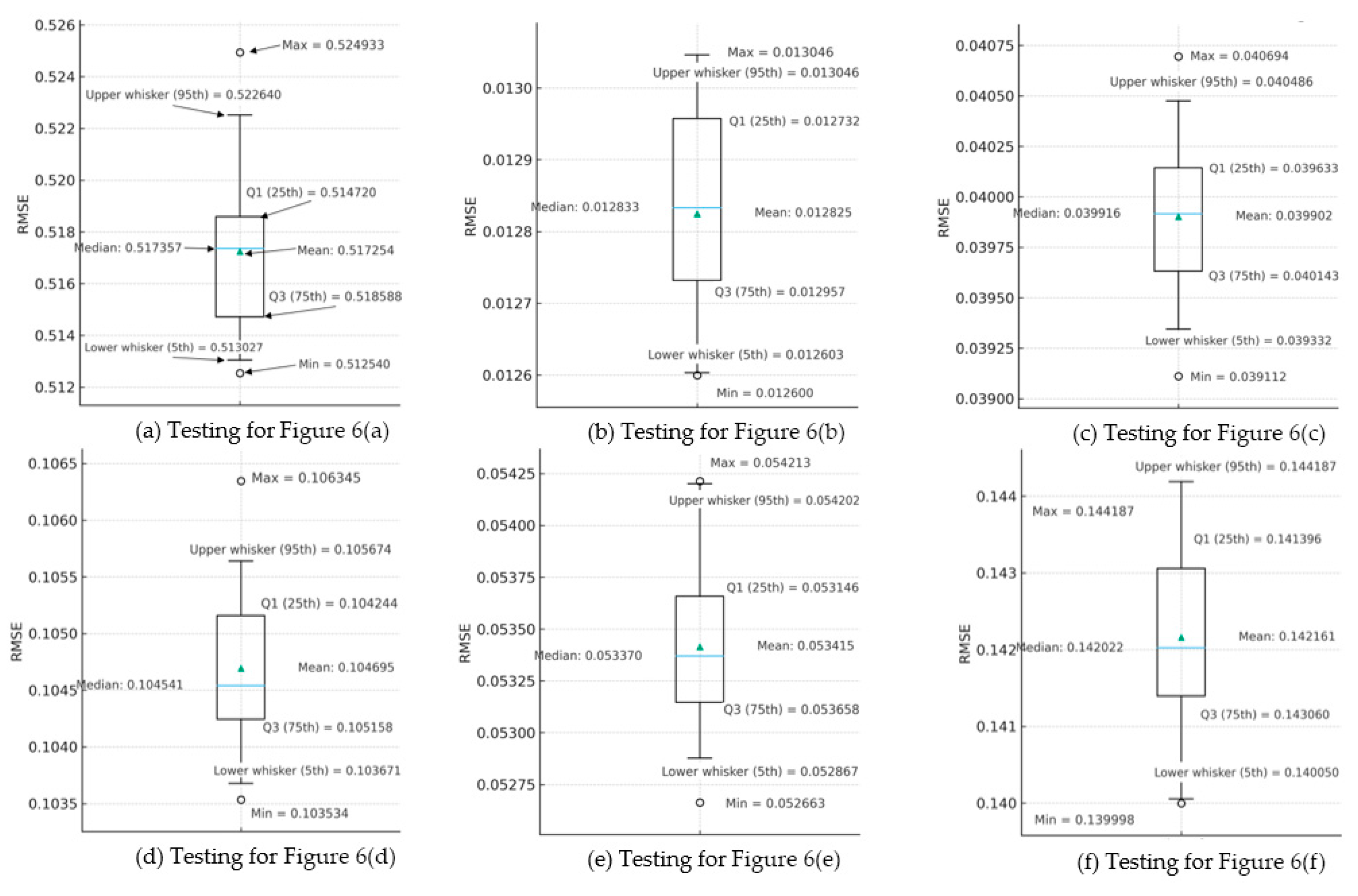
We ran 20 independent trials per model (Figure 6a–f) with different random seeds affecting (i) probabilistic knot sampling via D(u), (ii) mutation and population shuffling, and (iii) the initial ordering of individuals. All other hyperparameters were fixed (cubic B-splines, population W = 30, Max_iter = 50, target accuracy 10−3 Lmax, early stopping, etc.). We report point-to-surface RMSE using boxplots: the box spans [Q1, Q3], the line is the median, the triangle is the mean; whiskers denote the 5th–95th percentiles, with points beyond shown as outliers, as shown in Figure 13.
As shown in Figure 13, dispersion is small across all six models: the IQR-to-median ratio lies within 0.7–1.8%, the 95th percentile is within 1.7% above the median, and the 5th percentile within about 1.2% below it, with only a few outliers. This indicates high robustness to random initialization. We attribute it to the hybrid knot-guidance strategy, which provides high-quality and diverse starting populations, and to HPA’s global search with mutation, which avoids poor local minima.
It can be seen from the above experimental results that HPA has relatively higher search ability and efficiency, and is more stable. Moreover, the HPA can still maintain the diversity of the population after the iteration number reaches half and has a better ability to jump out of the local optimum. Especially in the case of knot guidance technology, when solving more complex engineering models, it can often obtain better fitting results under the same conditions.

5.2. Comparison with Commercial Software

The hull profile is a typical reverse engineering application, which determines the key characteristics of the ship, such as power and resistance, and can have a great impact on the key factors, such as ship construction efficiency and cost [48]. Therefore, the accuracy and smoothness of the hull profile design are extremely critical. At present, the mother-type transformation is the mainstream ship design method. According to the existing designs with similar functions, the hull is cut at different positions several times to form the ship form line diagram and offset table, including the cross-section, longitudinal section and waterline surface, as shown in Figure 14. On this basis, the new ship form is developed.
In this paper, a ship with a length of 189.98 m, a width of 32.26 m and a depth of 16 m is fitted, and the fitting effect is compared with the existing surface design software CATIA. The offset table and the shape line diagram are shown in Figure 15.
The walls on both sides of the ship are approximately flat, and the difficulty in fitting the hull profile lies in the bow and stern. Take the corresponding 25 ship longitudinal profile lines and take 25 × 134 data points, as shown in Figure 16.
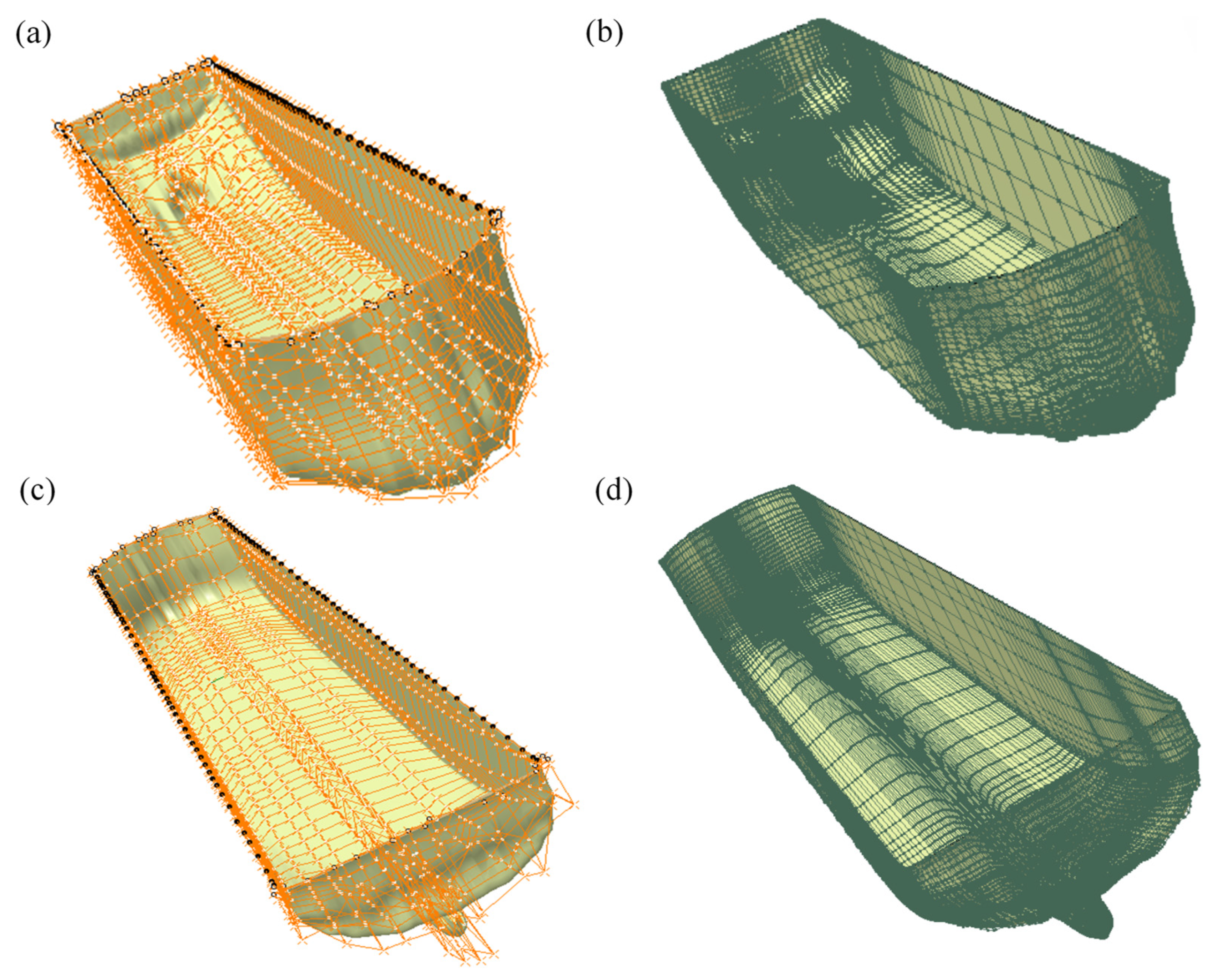
For ship design, the ship field requires that the design error of each profile line is 10−3, and the transition between profile lines is smooth. Under this condition, the HPA proposed in this paper uses a 58 × 21 mesh, while the CATIA control mesh number is 127 × 58, as shown in Figure 17.
It can be seen from the effect of ship fitting that for the same data points and the same fitting accuracy, the control mesh of HPA proposed in this paper is more compact than that of CATIA, which proves the superiority and effectiveness of HPA.

6. Conclusions

In this study, a B-spline surface fitting method based on the Hungry Predation Algorithm (HPA) was developed for efficient reverse modeling of industrial products. The method introduces a hybrid knot guidance strategy to improve initial knot placement and incorporates a hunger-inspired search mechanism to accelerate convergence while maintaining population diversity. Additionally, an adaptive parameter adjustment framework is designed to automate the selection of internal knot rates and algorithm parameters, reducing the need for manual intervention. Compared with traditional static and dynamic knot methods, as well as commercial CAD software such as CATIA, the proposed method achieves higher accuracy with fewer control points and faster computation time. HPA exhibits a strong generalization ability across a range of geometric complexities and demonstrates significant potential for practical application in engineering design and manufacturing.
For the hull datasets used in this study, the HPA-guided fitting already meets engineering turnaround requirements. Looking ahead, our priority is to further reduce computational cost and memory footprint for ultra-large, high-complexity point clouds. During computation, brute-force searches can be replaced with spatial indexes (KD-tree/BVH), lowering nearest-neighbor queries in point–surface distance evaluation from O (N2) to O (NlogN); B-spline basis functions and their derivatives can be cached; and the least-squares system assembled in sparse form and solved with sparse QR/SVD or preconditioned iterative methods (LSQR/CG), thereby reducing factorization cost and peak memory. Three levels of parallelism can be exploited: (i) population-level parallel updates of knot candidates; (ii) batched fitness evaluation across patches; and (iii) GPU acceleration of basis and distance kernels (optionally using mixed precision). Collectively, these measures can markedly reduce wall-time and memory usage on industrial-scale data while incurring only minimal accuracy loss.

Author Contributions

Conceptualization, M.L. and C.S.; methodology, M.L.; software, M.L.; validation, M.L. and S.G.; investigation, M.L.; resources, C.S.; data curation, M.L.; writing—original draft preparation, M.L.; writing—review and editing, M.L. and C.S.; funding acquisition, C.S. All authors have read and agreed to the published version of the manuscript.

Funding

This research was funded by National Key Research and Development Program grant number [2022YFC3006004].

Data Availability Statement

Data will be made available on reasonable request.

Conflicts of Interest

The authors declare no conflicts of interest, and there is no copyright issue for the figures.

References

  1. Park, H. B-spline surface fitting based on adaptive knot placement using dominant columns. CAD Comput. Aided Des. 2011, 43, 258–264. [Google Scholar] [CrossRef]
  2. Kawasaki, T.; Jayaraman, P.K.; Shida, K.; Zheng, J.; Maekawa, T. An image processing approach to feature-preserving B-spline surface fairing. CAD Comput. Aided Des. 2018, 99, 1–10. [Google Scholar] [CrossRef]
  3. Jiang, X.; Wang, B.; Huo, G.; Su, C.; Yan, D.M.; Zheng, Z. Scattered Points Interpolation with Globally Smooth B-Spline Surface using Iterative Knot Insertion. CAD Comput. Aided Des. 2022, 148, 103244. [Google Scholar] [CrossRef]
  4. Piegl, L.; Tiller, W. The NURBS Book (Monographs in Visual Communication); Springer: Berlin/Heidelberg, Germany, 1996. [Google Scholar]
  5. Yang, L.; Ran, C.; Yu, Z.; Han, F.; Wu, W. Surface Reconstruction and Volume Calculation of Grain Pile Based on Point Cloud Information from Multiple Viewpoints. Agriculture 2025, 15, 1208. [Google Scholar] [CrossRef]
  6. Luo, Y.; Li, S.; Ruan, J.; Bai, J. A Space Discretization Method for Smooth Trajectory Planning of a 5PUS-RPUR Parallel Robot. Appl. Sci. 2025, 15, 9212. [Google Scholar] [CrossRef]
  7. Suzuki, S.; Ohtake, Y.; Suzuki, H. Curvature Gradient-estimation Using CT Sinogram and its Application to Reverse Engineering. CAD Comput. Aided Des. 2022, 148, 103240. [Google Scholar] [CrossRef]
  8. Albrecht, G.; Mainar, E.; Peña, J.M.; Rubio, B. A Shape Preserving Class of Two-Frequency Trigonometric B-Spline Curves. Symmetry 2023, 15, 2041. [Google Scholar] [CrossRef]
  9. Kovács, I.; Várady, T. Constrained fitting with free-form curves and surfaces. CAD Comput. Aided Des. 2020, 122, 102816. [Google Scholar] [CrossRef]
  10. Liu, H.; Liu, Y.; Zhou, M.; Liu, L.; Liu, J.; Liu, Z.; Li, H.; Li, P. Research on 3D Modeling Method of Tunnel Surrounding Rock Structural Planes Based on B-Spline Interpolation. Appl. Sci. 2025, 15, 8142. [Google Scholar] [CrossRef]
  11. Dai, J.; Chai, Y.; Xiong, P. Path Planning of Underground Robots via Improved A* and Dynamic Window Approach. Appl. Sci. 2025, 15, 6953. [Google Scholar] [CrossRef]
  12. Zhou, H.; Shang, T.; Wang, Y.; Zuo, L. Salp Swarm Algorithm Optimized A* Algorithm and Improved B-Spline Interpolation in Path Planning. Appl. Sci. 2025, 15, 5583. [Google Scholar] [CrossRef]
  13. Sun, C.; Liu, M.; Ge, S. B-Spline Curve Fitting of Hungry Predation Optimization on Ship Line Design. Appl. Sci. 2022, 12, 9465. [Google Scholar] [CrossRef]
  14. Gálvez, A.; Iglesias, A. Particle swarm optimization for non-uniform rational B-spline surface reconstruction from clouds of 3D data points. Inf. Sci. 2012, 192, 174–192. [Google Scholar] [CrossRef]
  15. Gálvez, A.; Iglesias, A.; Puig-Pey, J. Iterative two-step genetic-algorithm-based method for efficient polynomial B-spline surface reconstruction. Inf. Sci. 2012, 182, 56–76. [Google Scholar] [CrossRef]
  16. Duan, Q.; Bao, F.; Du, S.; Twizell, E.H. Local control of interpolating rational cubic spline curves. CAD Comput. Aided Des. 2009, 41, 825–829. [Google Scholar] [CrossRef]
  17. Deng, C.; Lin, H. Progressive and iterative approximation for least squares B-spline curve and surface fitting. CAD Comput. Aided Des. 2014, 47, 32–44. [Google Scholar] [CrossRef]
  18. Crum, J.; Levine, J.A.; Gillette, A. Extending Discrete Exterior Calculus to a Fractional Derivative. CAD Comput. Aided Des. 2019, 114, 64–72. [Google Scholar] [CrossRef]
  19. Sánchez-Reyes, J.; Chacón, J.M. A polynomial Hermite interpolant for C 2 quasi arc-length approximation. CAD Comput. Aided Des. 2015, 62, 218–226. [Google Scholar] [CrossRef]
  20. Fauser, J.; Seelecke, S.; Werthschutzky, R.; Kupnik, M.; Mukhopadhyay, A.; Chadda, R.; Goergen, Y.; Hessinger, M.; Motzki, P.; Stenin, I.; et al. Planning for flexible surgical robots via bézier spline translation. IEEE Robot. Autom. Lett. 2019, 4, 3270–3277. [Google Scholar] [CrossRef]
  21. Lee, S.; Wolberg, G.; Shin, S.Y. Scattered data interpolation with multilevel b-splines. IEEE Trans. Vis. Comput. Graph. 1997, 3, 228–244. [Google Scholar] [CrossRef]
  22. Piegl, L.A.; Tiller, W. Least-squares B-spline curve approximation with arbitrary end derivatives. Eng. Comput. 2000, 16, 109–116. [Google Scholar] [CrossRef]
  23. Lyche, T.; Mørken, K. Knot removal for parametric B-spline curves and surfaces. Comput. Aided Geom. Des. 1987, 4, 217–230. [Google Scholar] [CrossRef]
  24. Razdan, A. Knot Placement for B-Spline Curve Approximation. Tech. Rep. Ariz. State Univ. 1999, 1, 8. [Google Scholar]
  25. Park, H.; Lee, J.H. B-spline curve fitting based on adaptive curve refinement using dominant points. CAD Comput. Aided Des. 2007, 39, 439–451. [Google Scholar] [CrossRef]
  26. Park, H.; Jung, H.B.; Kim, K. A new approach for lofted b-spline surface interpolation to serial contours. Int. J. Adv. Manuf. Technol. 2004, 23, 889–895. [Google Scholar] [CrossRef]
  27. Park, H. An approximate lofting approach for B-spline surface fitting to functional surfaces. Int. J. Adv. Manuf. Technol. 2001, 18, 474–482. [Google Scholar] [CrossRef]
  28. Lyche, T.; Morken, K. A date reduction strategy for splines. Ima J. Numer. Anal. 1988, 8, 185–208. [Google Scholar] [CrossRef]
  29. Jiang, B.; Han, J.; Tian, X.; Xia, L. B-spline surface fitting algorithm based on contour constraint points. China Mech. Eng. 2015, 26, 2016–2021. [Google Scholar]
  30. Yoshimoto, F.; Harada, T.; Yoshimoto, Y. Data fitting with a spline using a real-coded genetic algorithm. CAD Comput. Aided Des. 2003, 35, 751–760. [Google Scholar] [CrossRef]
  31. Sarfraz, M. Representing Shapes by Fitting Data using an Evolutionary Approach. Comput. Aided Des. Appl. 2004, 1, 179–185. [Google Scholar] [CrossRef]
  32. Gálvez, A.; Iglesias, A.; Avila, A.; Otero, C.; Arias, R.; Manchado, C. Elitist clonal selection algorithm for optimal choice of free knots in B-spline data fitting. Appl. Soft Comput. 2015, 26, 90–106. [Google Scholar] [CrossRef]
  33. Ülker, E.; Arslan, A. Automatic knot adjustment using an artificial immune system for B-spline curve approximation. Inf. Sci. 2009, 179, 1483–1494. [Google Scholar] [CrossRef]
  34. Ülker, E. B-Spline Curve Approximation Using Pareto Envelope-Based Selection, Algorithm—PESA. Int. J. Comput. Commun. Eng. 2013, 2, 60. [Google Scholar] [CrossRef]
  35. Valenzuela, O.; Delgado-Marquez, B.; Pasadas, M. Evolutionary computation for optimal knots allocation in smoothing splines. Appl. Math. Model. 2013, 37, 5851–5863. [Google Scholar] [CrossRef]
  36. Gálvez, A.; Iglesias, A. Firefly algorithm for explicit B-spline curve fitting to data points. Math. Probl. Eng. 2013, 2013, 528215. [Google Scholar] [CrossRef]
  37. Liu, G.; Wong, Y.; Zhang, Y.; Loh, H. Adaptive fairing of digitized point data with discrete curvature. CAD Comput. Aided Des. 2002, 34, 309–320. [Google Scholar] [CrossRef]
  38. Xu, S.; Guo, Y.; Qi, X.; Xia, W. Chaotic ant swarm optimization in solving curve fitting with free knot B-splines. Comput. Eng. Appl. 2014, 50, 177–182. [Google Scholar]
  39. Piegl, L.A.; Tiller, W. Surface approximation to scanned data. Vis. Comput. 2000, 16, 386–395. [Google Scholar] [CrossRef]
  40. Piegl, L.A.; Tiller, W. Reducing control points in surface interpolation. IEEE Comput. Graph. Appl. 2000, 20, 70–75. [Google Scholar] [CrossRef]
  41. KWeinert, T.; Surmann, J. Mehnen. Evolutionary Surface Reconstruction Using CSG-NURBS-Hybrids; University of Birmingham: Birmingham, AL, USA, 2001; pp. 1456–1463. [Google Scholar]
  42. Wagner, T.; Michelitsch, T.; Sacharow, A. On the Design of Optimisers for Surface Reconstruction. In Proceedings of the 9th Annual Conference on Genetic and Evolutionary Computation, London, UK, 7–11 July 2007. [Google Scholar] [CrossRef]
  43. Mirjalili, S.; Lewis, A. The Whale Optimization Algorithm. Adv. Eng. Softw. 2016, 95, 51–67. [Google Scholar] [CrossRef]
  44. Rashedi, E.; Nezamabadi-Pour, H.; Saryazdi, S. GSA: A Gravitational Search Algorithm. Inf. Sci. 2009, 179, 2232–2248. [Google Scholar] [CrossRef]
  45. Merino, D.I.; Reyes, E.N.; Steidley, C.W. Genetic algorithms: Theory and application. Comput. Educ. J. 2000, 10, 3–298. [Google Scholar] [CrossRef]
  46. Mirjalili, S.; Mirjalili, S.M.; Lewis, A. Grey Wolf Optimizer. Adv. Eng. Softw. 2014, 69, 46–61. [Google Scholar] [CrossRef]
  47. Storn, R.; Price, K. Differential Evolution—A Simple and Efficient Heuristic for Global Optimization over Continuous Spaces. J. Glob. Optim. 1997, 11, 341–359. [Google Scholar] [CrossRef]
  48. Son, M.J.; Kim, T.W. Implementation of an executable business process management model for the ship hull production design process. J. Mar. Sci. Technol. 2014, 19, 170–184. [Google Scholar] [CrossRef]
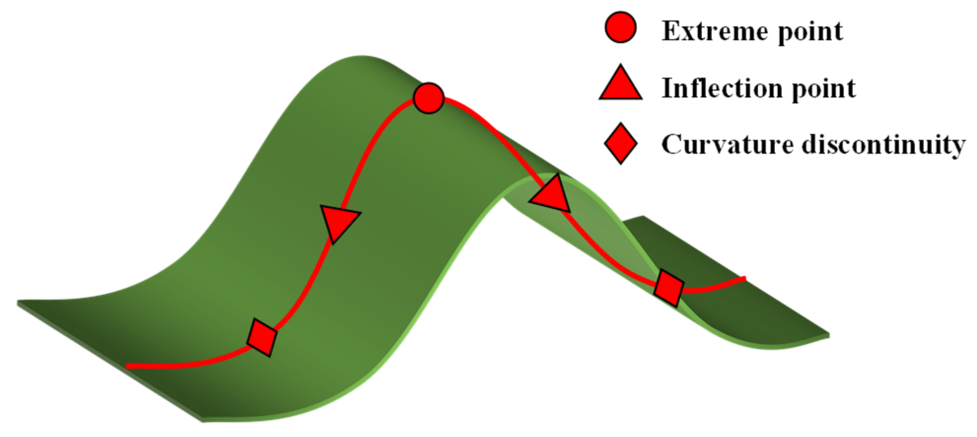
Figure 1. Feature points on the curve.
Applsci 15 11471 g001
Figure 2. Schematic diagram of Equation (6).
Applsci 15 11471 g002
Figure 3. Schematic illustration of Equation (8).
Applsci 15 11471 g003
Figure 4. HPA search schematic diagram.
Applsci 15 11471 g004
Figure 5. Main flow of HPA.
Applsci 15 11471 g005
Figure 6. Elementary analytical surface (a), simple free-form surface (b), face surface (c), human body surface (d), automobile outline (e), and ship outline (f).
Applsci 15 11471 g006
Figure 7. Influence of the variation rate of knot guidance technology on the results.
Applsci 15 11471 g007
Figure 8. The effect of decreasing W and Max_iter (a), and the effect of increasing both (b).
Applsci 15 11471 g008
Figure 9. Human body model data point cloud (a) and face model data point cloud (b).
Applsci 15 11471 g009
Figure 10. Fitting result and control mesh of HPA on human model under the tolerance rates of 10−2 (a) and 10−3 (b).
Applsci 15 11471 g010
Figure 11. Fitting effect of HPA on face model and its control mesh under the tolerance rates of 10−2 (a) and 10−3 (b).
Applsci 15 11471 g011
Figure 12. Comparison of the fitting effects of various optimization algorithms on the six models (af) mentioned in Figure 6.
Applsci 15 11471 g012aApplsci 15 11471 g012b
Figure 13. Algorithm robustness testing.
Applsci 15 11471 g013
Figure 14. Cross-section, longitudinal section and waterline surface of a ship.
Applsci 15 11471 g014
Figure 15. Offset table and line diagram of a ship.
Applsci 15 11471 g015
Figure 16. Data point extraction of longitudinal section profile.
Applsci 15 11471 g016
Figure 17. Fitting effect and control mesh of bow angle HPA (a) and CATIA (b) and stern angle HPA (c) and CATIA (d).
Applsci 15 11471 g017
Table 1. Comparison of the control mesh with relevant methods under the same accuracy.
Comparison 1 Control MeshComparison 2 Control Mesh
Traditional approach1080 × 21NKTP [39]43 × 26 (tolerance rate = 0.01)
Piegl and Tiller’s approach [40]89 × 21 (per = 1.00) 81×39 (tolerance rate = 0.001)
127 × 21 (per = 0.75)
168 × 21 (per = 0.50)DOM [1]23 × 22 (tolerance rate = 0.01)
292 × 21 (per = 0.25) 37 × 35 (tolerance rate = 0.001)
A new approach [26]78 × 21
HPA14 × 14 (tolerance rate = 0.01)HPA14 × 10 (tolerance rate = 0.01)
46 × 19 (tolerance rate = 0.001) 25 × 25 (tolerance rate = 0.001)
Table 2. Efficiency comparison with related optimization algorithms.
Ref.MethodPopulationData PointsErrorRuntime
[11]Neural network SOM and PDE with gradient descent algorithm (GDA)Not applicable10410−1–10−23–6 h
[12]Evolutionary algorithms (EA)30–50Not reportedNot reportedTens of minutes to hours
[41]Evolutionary search (ES) and genetic programming (GP)50019210−224 h
[42]Multi-objective evolutionary and genetic algorithm (MOEA)20823–17,30710−2Tens of hours to days
[15]Iterative two-steps genetic algorithm with SVD/LU mod LSQ fitting50–5006000–14,400<10−4Tens of seconds to 3 h
Our methodHPA201260–10,00010−1–10−3Tens of seconds to minutes
Table 3. Setting the basic parameters of each algorithm.
OptimizationGreedy AlgorithmParameter Settings
WOA×Parameter of logarithmic spiral b = 1
GSA×Initial value G0 = 100, Initial speed v0 = 0
EA×Crossover rate = 0.8, Mutation rate = 0.05
GWO×No parameters need to be set
HPA×Mutation rate of knots = 0.5, Hunger search rate = 0.6
PSO×Inertial coefficient W = 0.4, Initial speed v0 = 0.1
DEScale factor F = 0.5, Crossover rate = 0.5
Disclaimer/Publisher’s Note: The statements, opinions and data contained in all publications are solely those of the individual author(s) and contributor(s) and not of MDPI and/or the editor(s). MDPI and/or the editor(s) disclaim responsibility for any injury to people or property resulting from any ideas, methods, instructions or products referred to in the content.