AI-Based Decision Support System for Attenuating Traffic Congestion

Abstract

The transportation industry and transportation infrastructure are undergoing a profound transformation due to advances in the development of artificial intelligence (AI) algorithms that are not just a concept of the future but a reality. Advanced algorithms, predictive systems, and intelligent automation contribute to optimizing logistics, reducing costs, increasing safety, and reducing traffic congestion. AI is also used to optimize routes by analyzing multiple variables, such as distance, traffic, time constraints, and user preferences, to generate optimal routes between departure and destination points. Route planning systems can be integrated with real-time data on traffic, planned or unforeseen events, and other conditions that may affect the trip. AI algorithms can use this data to adapt routes and estimated arrival times based on changes in traffic or other conditions. The purpose of this article is to develop a model for predicting traffic flows at intersections based on historical and real-time data. The focus is on the genetic algorithm used to optimize a Long Short-Term Memory (LSTM) encoder–decoder. Specifically, the research aims to determine how well the proposed model performs when the data is optimized using the genetic algorithm. The results obtained for the proposed GA-LSTM show an average TTS reduction of −18.7%, a maximum improvement of −27.3%, an RMSE of 0.003587, and an MSE of 0.00348 compared to traditional models used in real time for traffic management. Finally, the performance of GA-LSTM was compared with the results reported in the literature to demonstrate the usefulness of the proposed algorithm.

1. Introduction

Current traffic management systems are based on three key elements: machine learning algorithms, neural networks, and optimization systems. Machine learning algorithms analyze historical data to discover patterns in traffic flows. Neural networks process information in real time to provide accurate predictions, and optimization systems make quick decisions to adjust traffic. AI traffic flow management is based on traffic pattern analysis, real-time traffic light control, navigation, and optimized routes. Traffic pattern analysis uses artificial intelligence-based systems that continuously monitor traffic flows to identify patterns useful for making quick decisions by developing predictive models that highlight traffic fluctuations, identify congested areas, and estimate the effects of various events. Real-time traffic light control is based on the models described above, contributing to congestion reduction and more efficient urban mobility, especially on major roads with heavy traffic. Navigation and optimized routing provide real-time alternative routes, avoiding congested areas and redistributing traffic more evenly. This integrated approach helps reduce delays and improve overall traffic flow.

According to United Nations estimates on global urbanization [1], 69% of the world’s population is projected to live in cities by 2050. Therefore, it is difficult to manage existing infrastructure and resources to provide viable urban living conditions for all citizens by achieving smart urban mobility. To achieve intelligent urban mobility (intelligent traffic), an important role is played by artificial intelligence (AI) algorithms and the fusion of data from traffic sensors [2,3].

Data fusion first appeared in the literature in the 1960s as a mathematical model for data manipulation [4]. It was first implemented in the USA in the 1970s, primarily in the fields of robotics and defense.

Intelligent transportation systems require reliable and accurate data for monitoring and managing operations that maximize safety and predict the efficiency of routes in the transportation system [5]. These must be collected in real time from the existing traffic on a stretch of road using sensors, which can include inductive loops, GPS, fixed detectors, microwave sensors (used for traffic at longer distances), radar, Bluetooth, and other types of sensors [6]. Traffic data has become a central and dominant element in every stage of road traffic management decision-making due to technological advancements [7]. The use of multiple methods for acquiring real-time field data can minimize the uncertainty errors that can arise when relying only on data obtained from individual sources. The algorithms used to develop intelligent transportation systems require a large amount of data obtained from a wide range of sensors, ensuring that the final predictions have a very low degree of error in traffic observation conditions.

Rapid progress is currently being made in the field of assisted and autonomous vehicles. Autonomous vehicles will soon be on public roads in increasing numbers. Due to the dynamic and complicated driving environment, autonomous cars face several obstacles [8]. Autonomous vehicles must predict future movements and adjust their behavior accordingly.

The car must choose between changing lanes, crossing intersections, and overtaking another vehicle. To achieve this, the vehicle must be able to predict the future movement of surrounding cars. Predicting the future trajectory is not a deterministic problem, as the driver’s goals and driving behavior vary. This suggests that several viable options are available for a similar driving scenario. The use of historical data facilitates the discovery of common solutions [9,10].

Existing trajectory planning algorithms are based on evaluating future trajectory conditions [11]. Most methods utilize an estimate of the vehicle’s motion state and a kinematic model to predict its future motion.

Motion-based models can replace kinematic models. Starting from a set of trajectory data, these models figure out how traffic dynamics change. They use recognition modules to determine how a given trajectory will unfold. The classifier receives information about the past (historical data) and the current motion state through recognition. For maneuver-based models, random forest classifiers and recurrent neural networks (RNNs) have been employed [12]. The biggest problem with these models is that they often lack high efficiency in modeling safety-critical motion patterns that were not included in the training data. Since motion prediction can be considered a sequence classification task, many classification methods based on RNNs have been proposed in recent years [13].

Deep learning models, including convolutional neural networks and recurrent neural networks, have been extensively applied in traffic forecasting problems to model spatial and temporal dependencies. In recent years, to model the graph structures in transportation systems as well as contextual information, graph neural networks (GNNs) have been introduced and have achieved state-of-the-art performance in a series of traffic forecasting problems. Even though GNNs are presented in the specialized literature as the future algorithm for traffic optimization, they also have several challenges in their implementation [14].

First, there is a significant error introduced by the small amount of data considered in existing GNN-based studies, which, in most cases, span less than a year. For this reason, the proposed solutions are not necessarily applicable to different time periods or different geographical locations. If very large traffic data are used in GNN, the corresponding change in traffic infrastructures should be recorded and updated, which increases both the expense and the difficulty of the associated data collection process in practice.

A second challenge is the scalability of GNN computation. To avoid the huge computational requirements of large-scale real-world traffic network graphs, only a subset of the nodes and edges is usually considered. Therefore, their results can only be applied to selected subsets. Graph partitioning and parallel computing infrastructures have been proposed to solve this problem, which can only run on a cluster with graphics processing units (GPUs).

A third challenge is the change in transportation networks and infrastructure, which is essential for building graphs in GNNs. Real-world network graphs change when road segments or bus lines are added or removed. Points of interest in a city also change when new facilities are built. Static graph formulations are not sufficient to handle these situations. GNNs can be combined with other advanced optimization techniques to overcome some of their inherent challenges and achieve better performance.

The objective of this study is to establish a comprehensive framework for predicting future trajectories utilizing historical data. This research primarily addresses the context of vehicular navigation on highways. The focus is centered on evaluating the efficacy of data processed through a genetic algorithm (GA), with the resultant output serving as input for an LSTM encoding–decoding framework. The assessment explicitly examines the system’s performance in relation to the data processed by the GA. Within the confines of the same LSTM framework, a comparative analysis is conducted of two primary methodologies. The first approach involves filtering the preprocessed dataset using the GA, followed by the integration of the filtered data into the LSTM framework.

In the article, we propose an algorithm composed of an LSTM neural network optimized with the genetic algorithm (GA) because road traffic prediction is based on time series analysis, and the LSTM neural network with short- and long-term memory is best suited for solving this problem. For the optimization of the LSTM, we chose the genetic algorithm (GA) to improve the accuracy of road traffic prediction and detection. GA can optimize the LSTM parameterization by generating hyperparameters regarding the number of hidden units, training times, and learning rate.

The remainder of this paper is as follows: Section 2 describes the materials and methods employed, including the architecture of the LSTM model, the genetic algorithm, and the proposed optimization framework. Section 3 presents the results obtained from the case study and simulation experiments, followed by a discussion of their implications. Finally, Section 4 summarizes the main conclusions and highlights directions for future research.

2. Materials and Methods

The approach combines deep learning techniques with evolutionary optimization, focusing on the integration of an LSTM neural network and a GA. First, the theoretical foundations of the LSTM model are introduced, with an emphasis on its ability to capture temporal dependencies in traffic flow data. Next, the principles and mechanisms of GA are described, highlighting its role in parameter optimization. Finally, the proposed hybrid architecture, which integrates both components, is outlined, illustrating how the combined model is designed to enhance prediction accuracy and computational efficiency.

2.1. Architecture of the Proposed Model

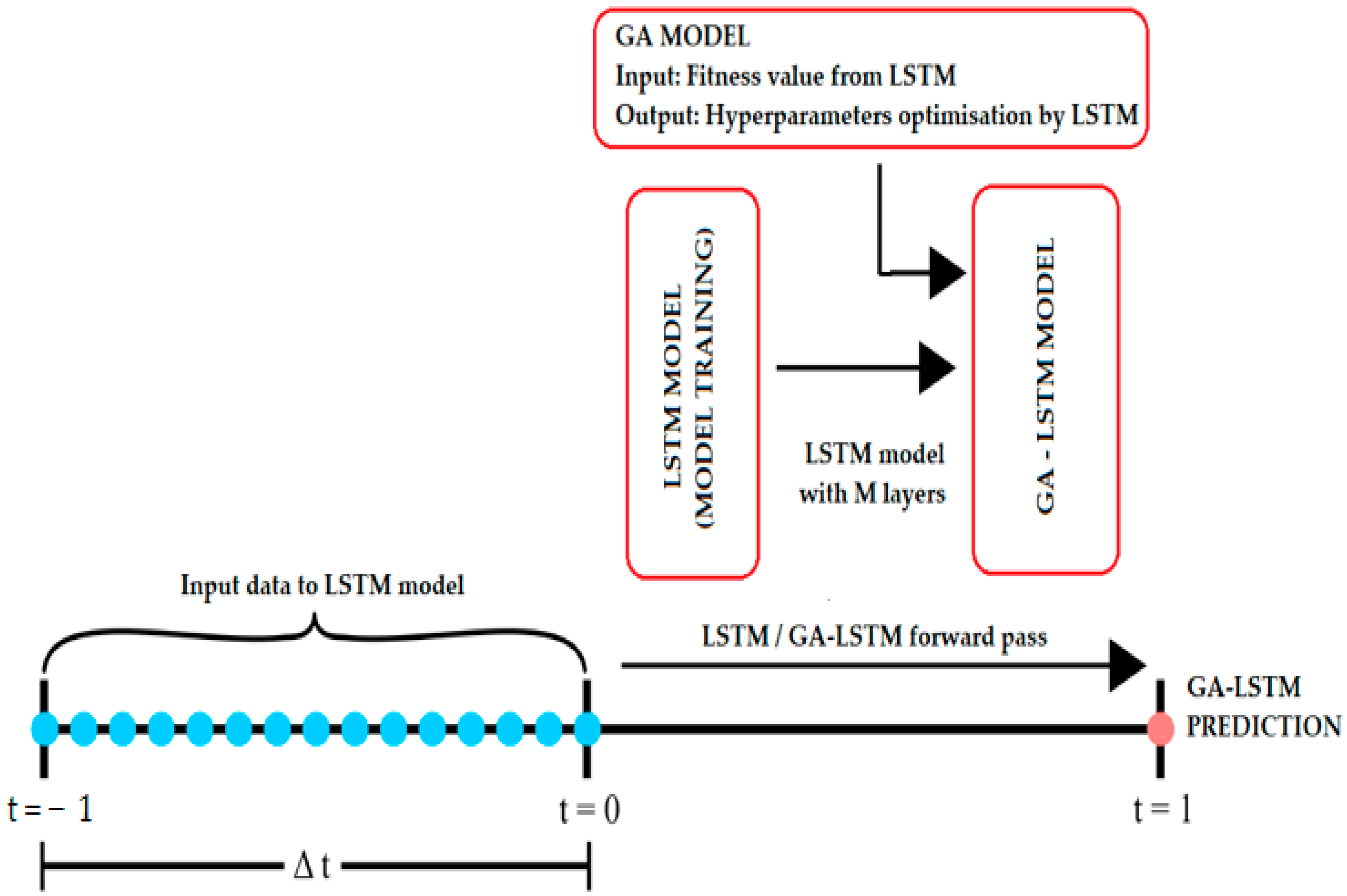
The proposed architecture for this study is shown in Figure 1. According to Figure 1, computational architecture consists of the following stages: historical and real-time data acquisition, data preprocessing and vectorization, feature identification and extraction, GA optimization to determine hyperparameters, and prediction using the LSTM algorithm.

The computational stages of the LSTM model with GA optimization are as follows:

• Data acquisition, preprocessing, and vectorization are achieved, and the models are trained using historical data.
• The mutation and crossover operators within the GA are optimized to obtain the best prediction models.
• The GA optimizes the output hyperparameters of the LSTM model based on the fitness parameters received from the LSTM model to optimize the process, thus achieving a biological evolution process. At this stage, the GA generates new populations through characteristic crossover, mutation, and replication operations, and solutions with low fitness are eliminated.
• The population generated by the GA is initialized and decoded, and the LSTM module uses the mean square error (MSE) as a fitness function. The fitness solutions from the LSTM and acquired by the GA support mutation and crossover selection operations.
• If the value of the fitness target function reaches an optimal value, the calculations continue; if the fitness value is small and must be eliminated, the calculations from the previous point are returned.
• If the fitness target value has optimal values, the prediction MSE is calculated based on the optimal prediction parameters.
• After calculating the set number of iterations of the GA, the calculation stops. At this point, the optimal combinations necessary for the LSTM model to make the final predictions are obtained.

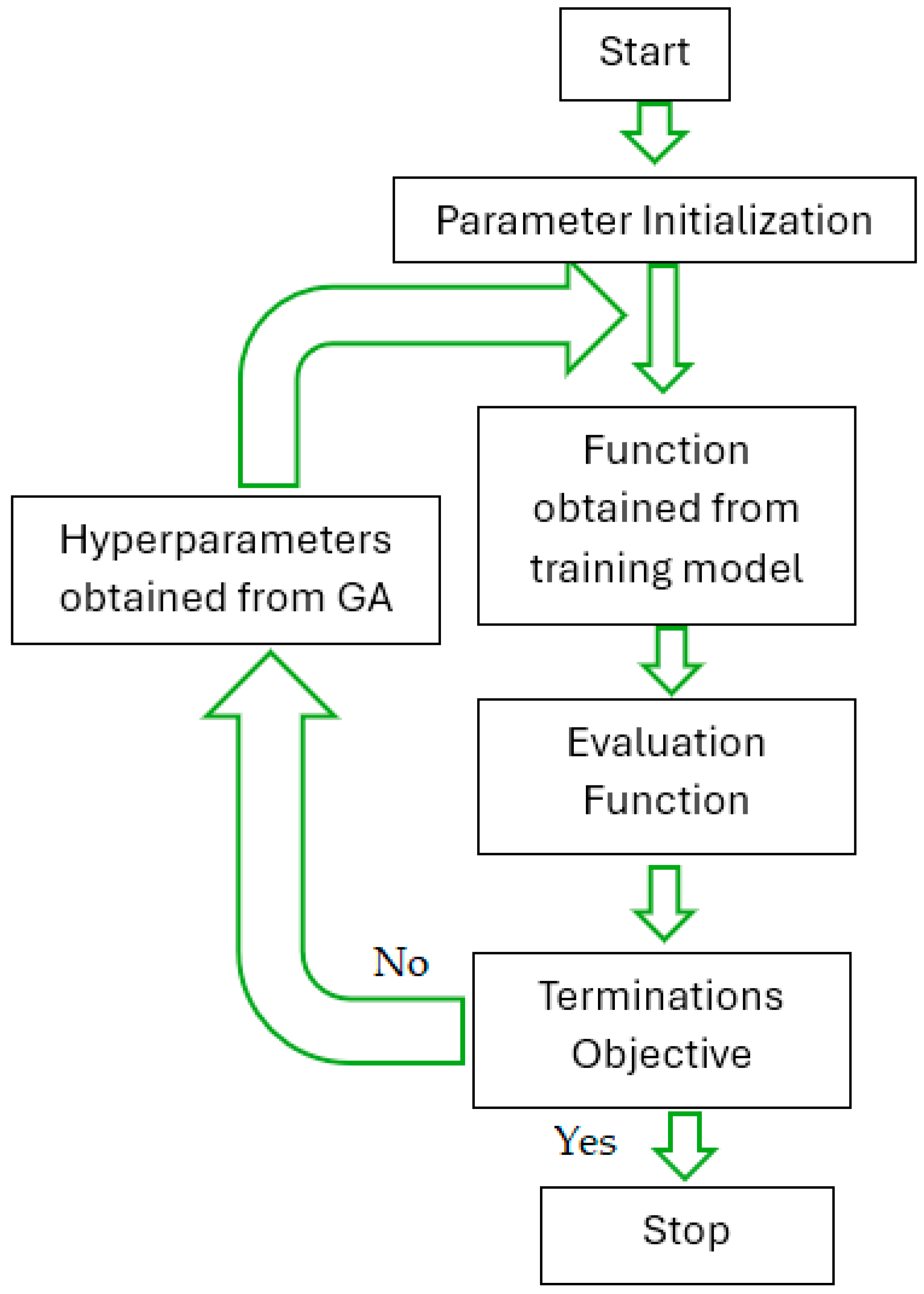
Genetic algorithm (GA) optimizes LSTM by automatically tuning its hyperparameters to improve prediction accuracy. GA will search for the optimal set of hyperparameters consisting of the number of hidden layers in the LSTM, the number of neurons in each LSTM layer, and the learning rate. The aim is to build an LSTM model that is more accurate than the initially chosen model. This set of hyperparameters is used for time series prediction, such as traffic flow prediction. Figure 2 shows the flow diagram for the proposed GA-LSTM.

To predict and simulate traffic behavior—including vehicle movement, interactions, and traffic flows—traffic optimization models are employed in various analytical and control applications. This study concentrates on modeling and controlling urban traffic flows.

Software simulators provide traffic analysis at macroscopic, mesoscopic, and microscopic levels to optimize the road network, reduce urban emissions, alleviate road congestion, and create urban environments suitable for vehicles and pedestrians. They can also realistically simulate complex interactions between vehicles at the microscopic level, model supply and demand and behavior in detail, simulate new forms of mobility, and ensure integration with other traffic planning tools [15,16].

The complexity inherent in these models allows for the consideration of diverse driver behaviors and the adjustment of parameters for specific vehicles. However, the detailed nature of these models can result in computational limitations that hinder real-time calculations within established time constraints. Traffic incidents represent a critical aspect of traffic studies, as they are predictive of road incidents based on traffic behavior, considering various traffic conditions and habits, such as vehicle flow, speed, and road occupancy. The occurrence of road incidents is closely associated with increased congestion, as incidents typically render roads unusable, thus exacerbating congestion in the vicinity.

The establishment of a dedicated response team is beneficial in emergency scenarios, facilitating efficient traffic management and mitigating prolonged congestion. Conversely, macroscopic traffic models delineate the behavior of groups of vehicles and overall vehicle flows rather than focusing on individual units. These models characterize vehicle flows in terms of average speed and density, which are essential for calculating traffic flows within networks. The behavior of a vehicle group is influenced by the traffic context surrounding it, particularly density. Some models in this category utilize look-up tables that correlate average density with average speed, although these tables vary across different intersections and networks, necessitating extensive data for effective application. Other models employ vehicle flows and throughputs to ascertain traffic movements within the network. Mesoscopic traffic models categorize vehicles based on shared behavioral characteristics. Such groupings are formed using probabilistic functions that allocate vehicles into distinct clusters displaying similar behaviors.

The parameters of individual vehicles can be represented through probability distributions centered around the mean values of their respective groups, thereby facilitating predictions regarding traffic flow across the network. A notable example of mesoscopic modeling is the gas kinetic model, which utilizes traffic density and equilibrium speed on a specified road segment to forecast vehicle speeds [17]. Enhancements to these models have been identified in store-and-forward (SFM) models, which operate based on state equations, with one state variable representing the number of vehicles on a roadway [18]. This model updates every second by accounting for vehicles entering and exiting the segment, thereby enabling a unified model applicable to all intersections within the system, regardless of temporal variations.

Transportation data fusion systems must effectively manage substantial communication loads to generate reliable and accurate outputs. At the macroscopic level, data fusion presents high complexity, particularly with heterogeneous data sources, such as diverse sensor outputs. The proposed data fusion or preprocessing methodology functions on collected data in its original state, involving processes of integration, association, and formatting to prepare the data for utilization in intelligent traffic systems. This preparatory layer employs various techniques, including noise reduction, outlier elimination, and the removal of abrupt spikes. The approach articulated in this paper introduces the utilization of LSTM-GA for preparing data from aggregated batches, thereby ensuring that the processed data is suitably structured for input into the selected traffic models [19].

2.2. Theoretical Approach of LSTM

RNNs are part of the concept of deep learning (DL) architecture and were designed for managing and analyzing data from time series models. LSTM is a type of artificial neural network that is used in the fields of deep learning and artificial intelligence. LSTM neural networks have feedback connections, unlike more traditional neural networks [20]. A recurrent neural network of this type can analyze not only individual data points but also multiple sequences of data [21].

Short-term memory models data from time series models by augmenting state vectors h and c, which will be trained to encode data about the phenomenon to be studied. Equations (1)–(6) describe an LSTM layer.

$${\mathrm{f}}_{\mathrm{t}}=\sigma \left({\mathrm{W}}_{\mathrm{f}}{\mathrm{x}}_{\mathrm{t}}+{\mathrm{U}}_{\mathrm{f}}{\mathrm{h}}_{\mathrm{t}-1}+{\mathrm{b}}_{\mathrm{f}}\right),$$

(1)

$${\mathrm{i}}_{\mathrm{t}}=\sigma \left({\mathrm{W}}_{\mathrm{i}}{\mathrm{x}}_{\mathrm{t}}+{\mathrm{U}}_{\mathrm{i}}{\mathrm{h}}_{\mathrm{t}-1}+{\mathrm{b}}_{\mathrm{i}}\right),$$

(2)

$${\mathrm{o}}_{\mathrm{t}}=\sigma \left({\mathrm{W}}_{\mathrm{o}}{\mathrm{x}}_{\mathrm{t}}+{\mathrm{U}}_{\mathrm{o}}{\mathrm{h}}_{\mathrm{t}-1}+{\mathrm{b}}_{\mathrm{o}}\right),$$

(3)

$${\tilde{\mathrm{c}}}_{\mathrm{t}}=\mathrm{t}\mathrm{a}\mathrm{n}\mathrm{h}\left({\mathrm{W}}_{\mathrm{c}}{\mathrm{x}}_{\mathrm{t}}+{\mathrm{U}}_{\mathrm{c}}{\mathrm{h}}_{\mathrm{t}-1}+{\mathrm{b}}_{\mathrm{c}}\right),$$

(4)

$${\mathrm{c}}_{\mathrm{t}}={\mathrm{f}}_{\mathrm{t}}°{\mathrm{c}}_{\mathrm{t}-1}+{\mathrm{i}}_{\mathrm{t}}°{\tilde{\mathrm{c}}}_{\mathrm{t}},$$

(5)

$${\mathrm{h}}_{\mathrm{t}}={\mathrm{o}}_{\mathrm{t}}°\mathrm{t}\mathrm{a}\mathrm{n}\mathrm{h}\left({\mathrm{c}}_{\mathrm{t}}\right),$$

(6)

where σ is the sigmoid activation function, which, together with the function tanh representing the hyperbolic tangent, is applied to each element of the state vector; the operator (°) represents the Hadamard product that is used for each component; $f_t$ represent the forgetting threshold layer; the output threshold layer is $o_t$; and $W_f$, $b_f$, $W_i$, $b_i$, $W_o$, $b_o$ are the weight and offset of each threshold layer, respectively.

The size of the state vectors, also referred to as units, determines the complexity of the LSTM architecture that can be modeled. Additionally, the complexity of the LSTM architecture can be augmented by increasing the number of LSTM layers relative to the desired model. In the context of LSTM models, the expansion of storage capacity for the RNN is facilitated through the utilization of single-unit states and threshold layers [22]. During the training process, the weights and biases of each threshold layer are derived from the historical dataset, enabling the model to identify and encode the characteristics inherent in the training data. In the inference phase, the predicted values of the time series are obtained by applying the trained model to the input data [17]. This study utilized TensorFlow [23] and Keras [24] to train traffic prediction models designed for traffic smoothing, which were subsequently implemented within the NI LabVIEW Real-Time development environment. 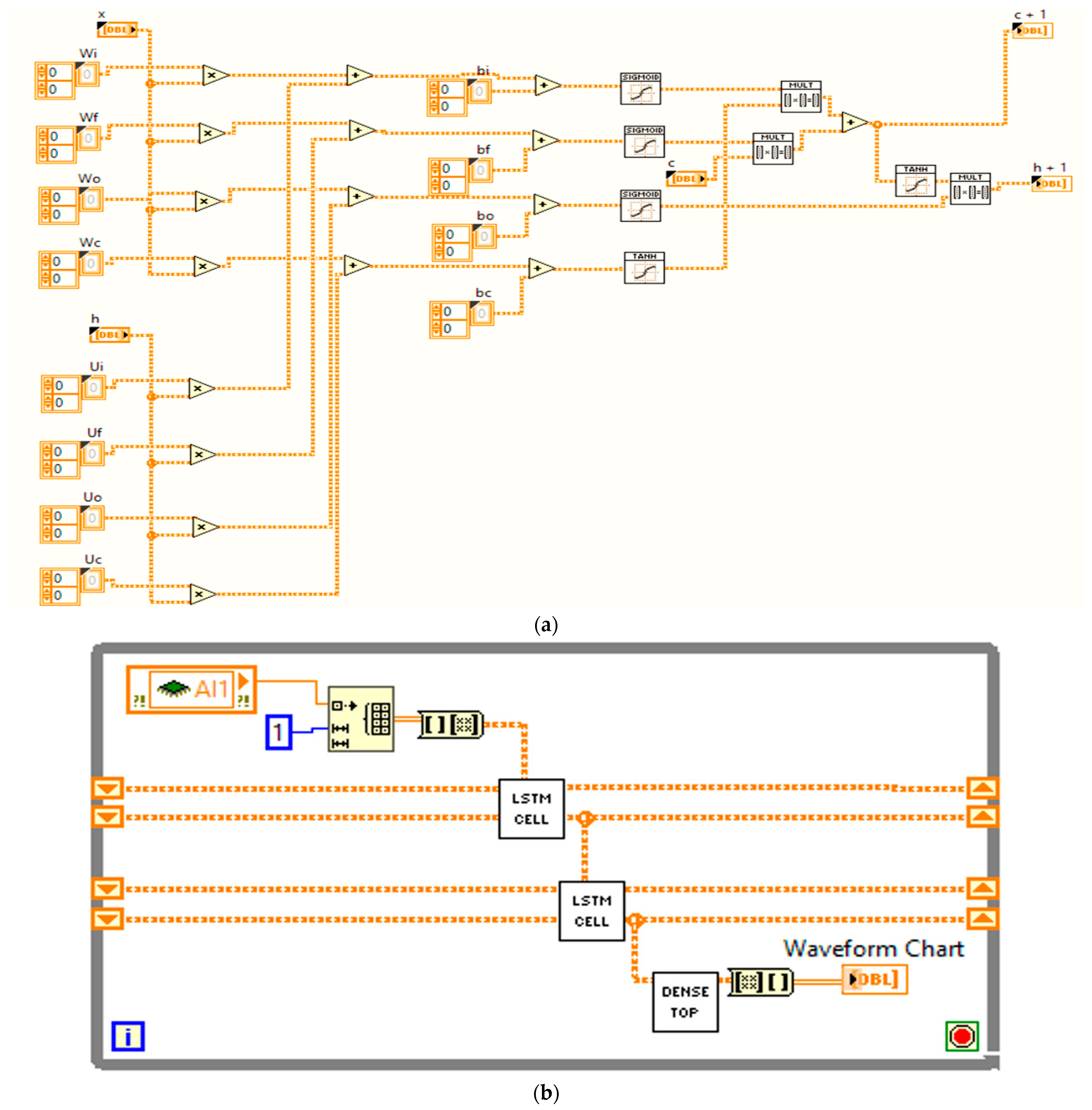Figure 3 illustrates the software implementation of the LSTM in LabVIEW, as described by Equations (1)–(6).

2.3. Genetic Algorithm Description

Genetic algorithms are part of the category of evolutionary computing algorithms and are inspired by Darwin’s theory of evolution [25]. Genetic algorithms start from an initial set of possible solutions to the problem (usually chosen randomly), called a “population” in the literature. In this population, everyone is called a “chromosome” and represents a possible solution to the problem. In almost all cases, the chromosome is a string of symbols (usually represented as a string of bits). These chromosomes evolve over successive iterations called generations. In each generation, the chromosomes are evaluated using some fitness measures. To create the next population, the best chromosomes from the current generation (population) are selected, and new chromosomes are formed using one of the three essential genetic operators: selection, crossover, and mutation [26].

Genetic algorithms have two main components that depend on the problem being addressed: the problem encoding and the evaluation (fitness) function. The chromosomes that represent the problem encoding must, to some extent, contain information about the solution to the problem and depend greatly on the problem. Several encodings have been used successfully, such as binary encoding (the chromosome is made up of strings of 0 or 1 that binary represent the solution to the problem) or value encoding (the chromosome is made up of a string of integer or real vector values that collectively represent the solution to the problem) [27,28].

The evaluation function, also called the “fitness” function, is the function that allows us to give confidence to each chromosome in the population. This function is usually the function that represents the description of the problem.

Another important step in the genetic algorithm is how we select the parents from the current population that will make up the new population. This can be achieved in several ways, but the basic idea is to select the best parents (in the hope that they will produce the best children). A problem may arise in this step: making the new population only based on the new children obtained can lead to the loss of the best chromosome obtained up to that step. Usually, this problem is solved using the so-called “elitism” method. That is, at least one chromosome that produces the best solution according to the fitness function is copied without any modification to the new population so that the best solution obtained up to that moment is not lost.

The operators of the genetic algorithm are selection, mutation, and crossover.

Selection: For this genetic operator, usually only one chromosome is selected from the population. This chromosome is copied to the new population without any modification. This method is also used to ensure that the chromosome that obtained the best value in the evaluation function (elitism) in the current population is not lost. This operator is also applied to other chromosomes selected based on the proposed selection methods, but usually this operator appears a small number of times when generating the new population.

Mutation: Mutation is another important genetic operator and represents the process by which the current chromosome occasionally changes one or more of its values in a single step. Mutation also depends on the coding of the chromosome. Mutation chooses only one candidate and randomly changes some of its values (changing only the sign of that value; sometimes the value is also changed, such as in the case of value representation, while sometimes only the value is changed, such as in the case of binary representation). Mutation works by randomly choosing the number of values to be changed and the way to change them.

Crossover: This operator depends very much on the type of chromosome encoding. The crossover method is applied to a pair of parents chosen using one of the presented methods. With probability, the parents are recombined to form two new offspring that will be introduced into the new population. For example, we take 2 parents from the current population, divide them, and cross the components to produce 2 new candidates. These candidates, after crossing, must represent a possible solution for the parameters of our optimization problem, so usually, values at the same positions are swapped. Using a recombination point, we can create new candidates by combining the first part of the first parent with the second part of the second parent. After recombination, a mutation can be randomly made on the new candidates obtained. If the chromosome size is large, more recombination points can be chosen [29].

When defining the parameters for the genetic algorithm, it is essential to consider both the population size and the number of parents. A greater number of parents can lead to increased variation in their offspring, depending on the method of selection employed. However, having too many parents may also diminish the efficiency of the selection algorithm and increase computational time. Similarly, while a larger population size results in more offspring and enhances the likelihood of obtaining viable genetic material, it also comes with the drawback of longer computation times.

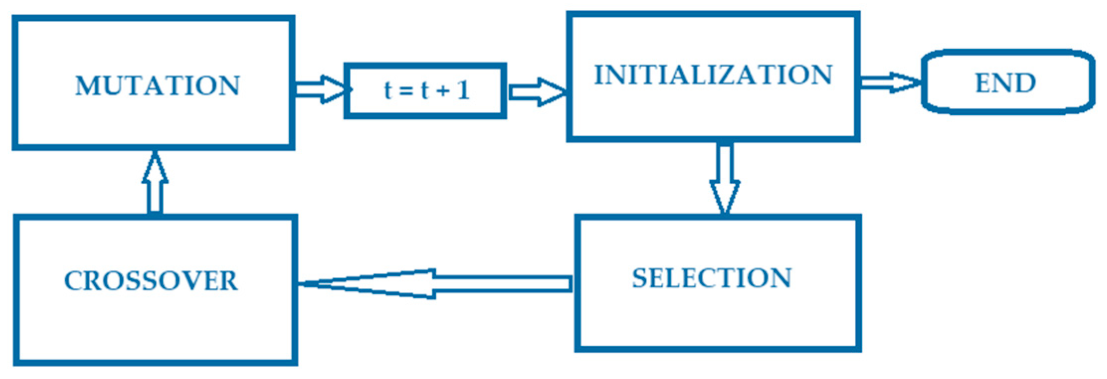
For modeling the urban traffic network (an intersection with multiple traffic flows), an average of the green times associated with traffic lights is used. This is because using more green times will negatively influence the efficiency of the genetic algorithm. Figure 4 shows the main stages of GA.

According to Figure 4, the operation of GA has four main stages:

• Initialization: Initialization of the elements needed to start the algorithm.
• Selection: This module selects chromosomes from the population for reproduction by evaluating them using the fitness function. The better the chromosome fits the task, the more times it can be selected.
• Crossover: Two individuals and a random point are selected, and the parents are eliminated; finally, their tails are crossed. For example, for 100110 and 111001, position three, from left to right, is selected, and they are crossed; the offspring are 100001 and 111110.
• Mutation: A gene, represented by a bit (in certain situations, the representation can be obtained on several bits), is randomly added to a chromosome. Nevertheless, the probability of this happening is minimal because, in this situation, the population can enter into chaotic disorder.

A fitness function is usually used to explicitly measure the performance of chromosomes, although in some cases, fitness can be measured implicitly using information about the performance of the systems. Chromosomes in a GA (Genetic Annotation—Group Action) take the form of strings of bits; they can be seen as points in the search space. This population is processed and updated by the GA, which is mainly driven by a fitness function, a mathematical function, a problem, or, in general, a specific task in which the population is to be evaluated.

It could be the case that a function to be optimized is available, and we will just need to program it. But for many problems, it is not easy to define an objective function. In such a case, we may use a set of training examples and define fitness as an error-based function. These training examples should describe the behavior of the system as a set of input/output relations. Considering a training set of k examples, we may have $\left(x_i,y_i\right), i=1, \dots ,k$, where $x_i$ is the input of the i-training sample, and $y_i$ is the corresponding output. The set should be sufficiently large to provide a basis for evaluating programs over several different significant situations. The fitness function may also be defined as the sum of the squared errors; it has the property of decreasing the importance of small deviations from the target outputs. If we define the error as $e_i={\left(y_i-o_i\right)}^2$, where $y_i$ is the desired output and $o_i$ the actual output, then the fitness will be defined as ${\sum }_{i=1}^k{e}_k={\sum }_{i=1}^k{\left(y_i-o_i\right)}^2$. The fitness function may also be scaled, thus allowing amplification of certain differences [30].

The stopping criteria determine what causes the algorithm to terminate. You can specify the following options:

• MaxGenerations: Specifies the maximum number of iterations that the genetic algorithm can perform. The default is 100$\ast$numberOfVariables.
• MaxTime: Specifies the maximum time in seconds that the genetic algorithm runs before stopping. This limit is applied after each iteration so that GA can exceed the limit when an iteration takes a substantial amount of time.
• FitnessLimit: The algorithm stops if the best fitness value is less than or equal to the FitnessLimit value.

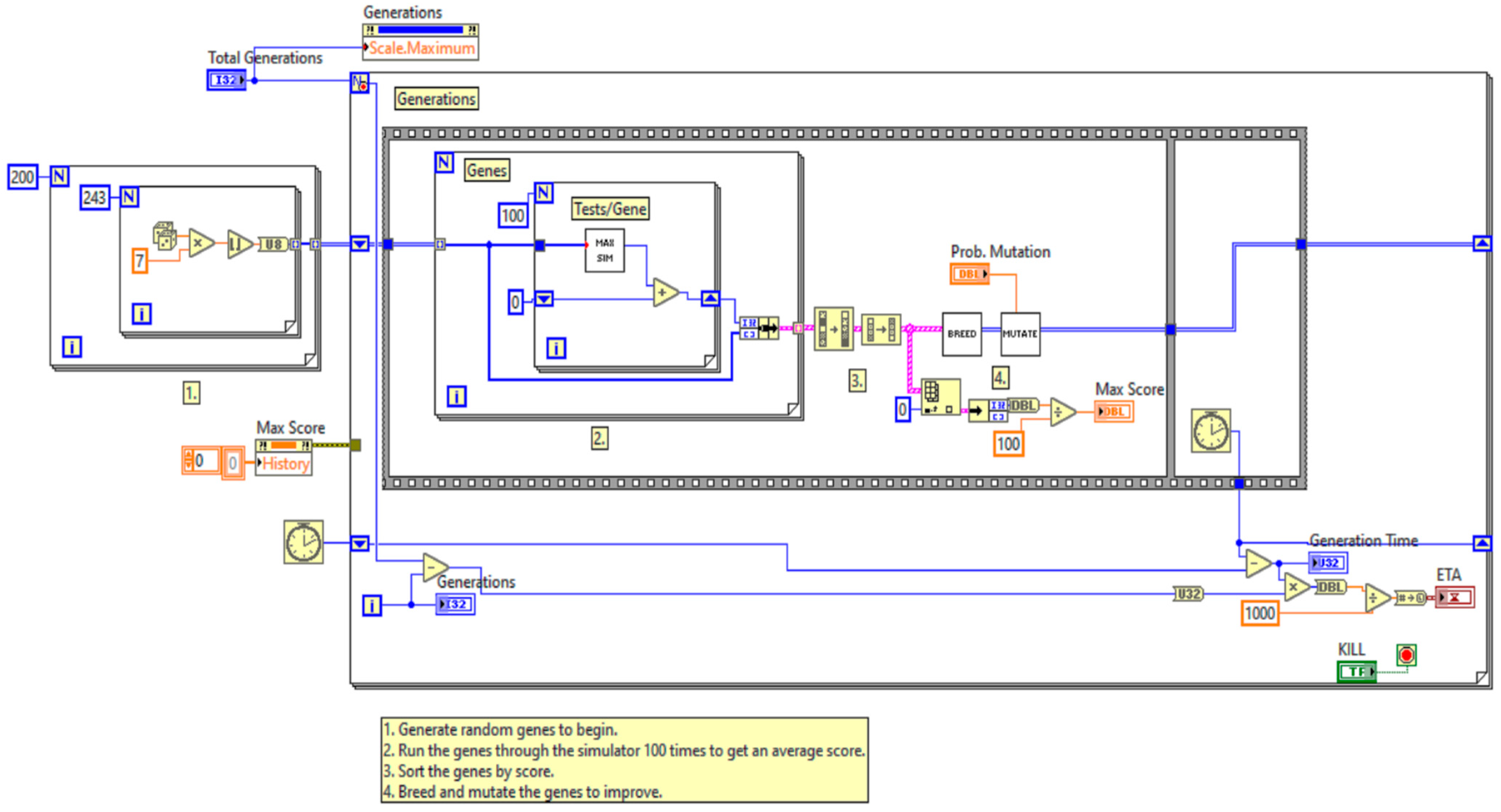
Figure 5 presents the LabVIEW-based implementation of GA, where each functional block corresponds to the algorithmic stages shown in Figure 4.

The initialization block sets the parameters and population, while the selection block evaluates chromosomes using the fitness function. In contrast, the crossover and mutation blocks create new candidate solutions by merging and modifying the selected parents. This graphic programming approach enables a clear visualization of genetic algorithm operations, making it easier to adjust parameters and monitor performance throughout the optimization process.

3. Results

The results include both quantitative metrics, such as computation time and prediction accuracy, as well as qualitative insights derived from the comparative evaluation of optimization algorithms. First, the research focused on modeling traffic through the application of queuing theory, which is a mathematical approach to analyzing waiting lines (queues). The advantage of employing this methodology lies in its capacity to facilitate predictions regarding queue lengths and waiting times. However, it is essential to note that the system’s stability is not guaranteed under all conditions.

In the analysis of vehicular traffic systems, stability is contingent upon the relationship between the rates of vehicle entry and exit. Specifically, when the rate of exiting vehicles surpasses that of entering vehicles, the system is deemed stable. This can be quantitatively described using the Poisson distribution parameter (p), where a condition of p < 1 indicates that the arrival rate is lower than the exit rate. Under such circumstances, the likelihood of traffic congestion at intersections is diminished. Conversely, when the arrival rate is greater than or equal to 1, it exceeds the exit rate, leading to the formation of prolonged queues and the subsequent emergence of traffic jams, which result in system instability. Consequently, maintaining the condition p < 1 is essential for ensuring system stability in traffic flow management.

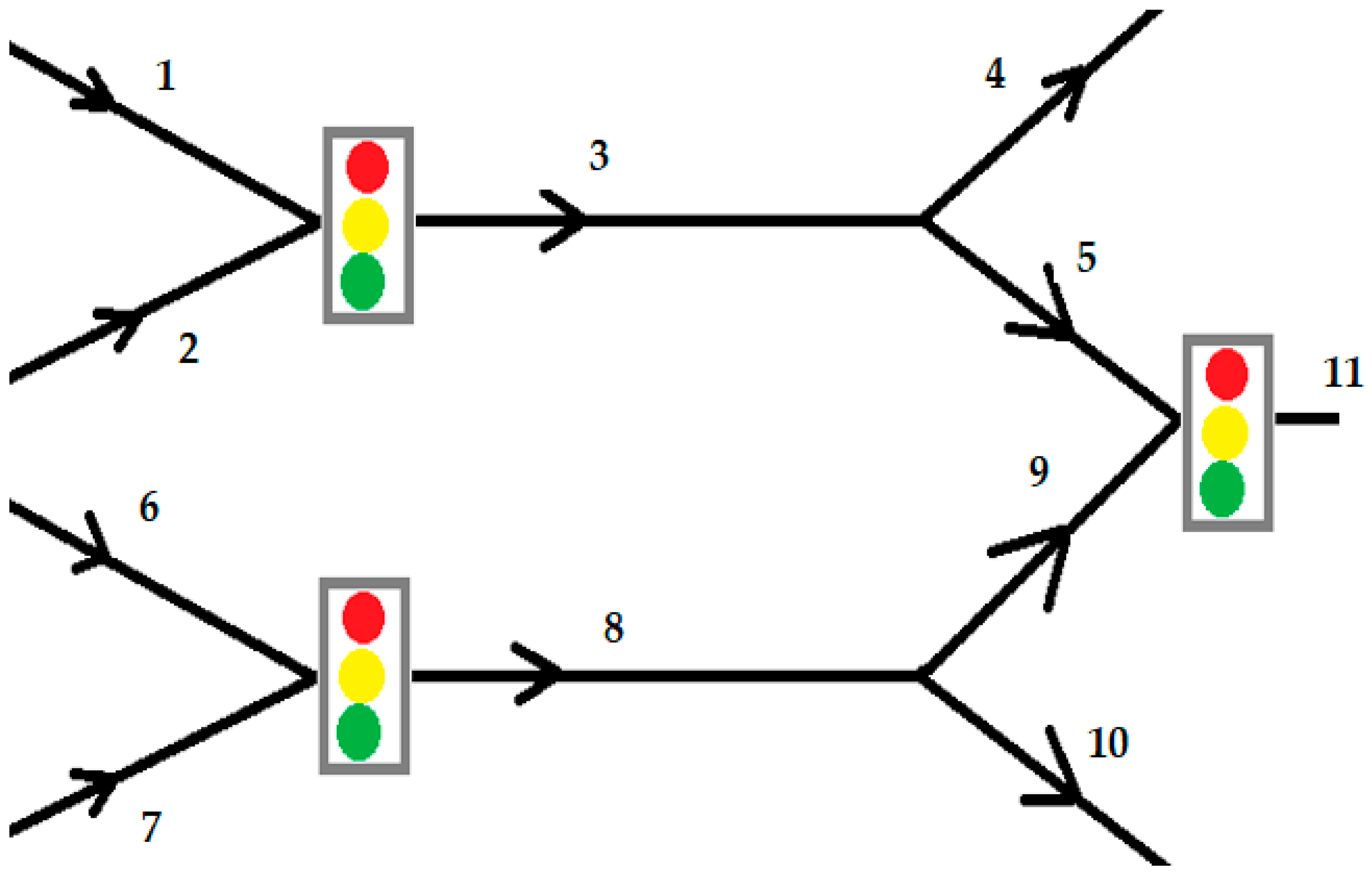
Secondly, an urban traffic network was selected to evaluate the efficacy of the LSTM model integrated with GA optimization for the purpose of optimizing traffic lights and enhancing traffic prediction accuracy. The urban traffic network utilized for this analysis is depicted in Figure 6, comprising three traffic light intersections.

The traffic network under consideration comprises eleven links, each structured as a one-lane, one-way street to facilitate a simplified model. The traffic simulation used has four entry routes (identified by traffic flows marked 1, 2, 6, and 7) and three exit routes (identified by traffic flows marked 4, 10, and 11). At the junctions, when the traffic lights are green, vehicles in the queue flow, and 3 and 8 leave the traffic through the exit routes.

Each link is associated with a defined turn rate, denoted as β_i,j, where i represents the link where vehicles are queued, and j signifies the link to which vehicles will depart. This turn rate quantifies the proportion of vehicles destined for link j relative to the total number in the queue.

For simulating real-time traffic conditions, the SUMO (Simulation of Urban Mobility) software was employed [31]. SUMO offers an extensive range of traffic scenarios designed to address vehicle flow patterns based on established car tracking models. The outcomes from these simulations are intended for analysis within the LabVIEW and MATLAB programming environments to evaluate the effectiveness of the proposed algorithm.

The SUMO traffic simulation software application allows data export to the MATLAB development program, and through the MathScript module (toolkit), data can be imported/exported to the LabVIEW development program. Using LabVIEW and MATLAB development programs simultaneously, the computing power for simulations that require complex mathematical algorithms can be increased.

The SUMO model was run in the first stage with 31 cycles for the first scenario and 14 cycles for the other three scenarios, waiting for traffic to be created on the links in the proposed network (Figure 6). The simulated model depends on the vehicle flow saturation rate μ, which is approximately 0.37 [veh/s], representing approximately 22 vehicles for a given cycle. Considering that only 60% of the vehicles go from link 3 to link 5 and 40% from link 8 to link 9, the number of vehicles reaching the second controlled intersection (links 5 and 9 traveling towards link 11) can be eliminated in a few cycles. Considering this network characteristic, we ran the scenarios for 30 sampling cycles of the traffic optimization control. After this time, the congestion has mostly disappeared at the intersection near the end of the network. The inbound links (at least some of them) are over-congested in most scenarios, so traffic optimization control is always necessary.

Simulations were conducted on a desktop computer equipped with an Intel Core i5-5300U processor and 10 GB of RAM, operating on the Windows 10 Pro platform. Version 1.21.0 of the SUMO traffic simulation software was used. The case study utilized an average travel speed reflective of conditions in Bucharest, Romania, established at 30 km/h, equating to 1 km per 2 min. Considering that the maximum speed limit for urban road segments is typically capped at 50 km/h, the chosen speed for this study was confined between 30 and 50 km/h.

Four distinct scenarios were formulated for the case study, each designed to induce congestion in various segments of the traffic network, thereby facilitating the observation of the impacts of traffic optimization via the LSTM-GA.

The SUMO simulation ran the 31-calculation subroutine for the first scenario and the 14-calculation subroutine for the next three scenarios, and finally, a significant amount of traffic was obtained for the network shown in Figure 6.

The determination of cycles necessary for simulations without GA optimization depends on the duration required to generate significant congestion based on input vehicle flow data and the predetermined green times of traffic signals. These green times were strategically set to ensure that at least one of the two links at the intersection experiences congestion.

Given that 60% of vehicles transition from link 3 to link 5 and 40% from link 8 to link 9, the traffic flow to the second controlled intersection (comprising links 5 and 9, which lead to link 11) can be adequately stabilized within a limited number of cycles. Considering this network characteristic, the execution of the scenarios was maintained over a span of 30 sampling cycles.

For this case study, the following scenarios were delineated according to Figure 6:

• Scenario 1: Links 1 and 5 are fully congested, links 2 and 6 exhibit high vehicle density, while links 7 and 9 are nearly devoid of traffic.
• Scenario 2: Links 1, 2, and 6 are completely congested. Link 7 shows minimal traffic, link 5 is congested, and link 9 is also nearly empty.
• Scenario 3: Links 2, 6, and 7 are entirely congested. In contrast, link 1 is almost devoid of vehicles, link 9 experiences congestion, and link 5 is nearly empty.
• Scenario 4: Links 1 and 9 are occupied by vehicles up to 50% of their capacity. Link 6 is occupied by a limited number of cars, approximately 25% of its capacity, while the remainder of the link remains free.

It should be noted that links 3 and 8 cannot experience congestion under the condition that either link 5 or link 9 is fully congested. For the proposed model, output nodes 4, 10, and 11 will not be crowded because they have direct outputs to other connections, according to Figure 6.

The extension of the LSTM capacity was achieved through the threshold layer and the single unitary state. In the training stage of the LSTM, the offsets and weights of each threshold layer were trained from the historical dataset so that it can identify and memorize historical state features. The processed and normalized data sequences were introduced into the proposed GA-LSTM to train the system. To run the application, we set the population individuals value to 50, the number of iterations to 30 and subsequently to 100, the variation rate and crossover probability to 0.006, the number of initially hidden unitary layers of the LSTM model to 5–100, the number of training epochs to 200 iterations, the initial value of the dropout layer to 0.15, the time step to 1–9, and the number of steps to 2.

To train the LSTM network, a database of real traffic data from Bucharest was created for 5 days (traffic from Monday to Friday). The training dataset consisted of 4 days, and the test dataset consisted of data from the 5th day. The parameters regarding the root mean square error (RMSE) and the mean square error (MSE) were used to evaluate the prediction. The following algorithms were used for comparative testing: LSTM, GA-BP (genetic algorithm with backpropagation network), fuzzy-logic BP, and the proposed GA-LSTM. The results obtained are presented in

Table 1. Results obtained for GA-LSTM prediction on working days.

MODEL	RMSE	MSE
LMSE	0.003512	0.1463
GA-BP	0.00479	0.00854
FUZZY-BP	0.00565	0.02357
GA-LSTM	0.003328	0.00431

.

According to the results presented in Table 1, the performance of LSTM deep learning compared to classic BP neural networks is better. In addition, the previous calculations were performed again for the weekend period. The results for the 2-day weekend are presented in

Table 2. Results obtained for GA-LSTM prediction on the weekend.

MODEL	RMSE	MSE
LMSE	0.004788	0.00586
GA-BP	0.005637	0.0155
FUZZY-BP	0.004965	0.0172
GA-LSTM	0.004548	0.00543

. According to the results presented in Table 2, the prediction for the weekend period is lower than for the weekday period, but the proposed GA-LSTM model has the best results in terms of prediction.

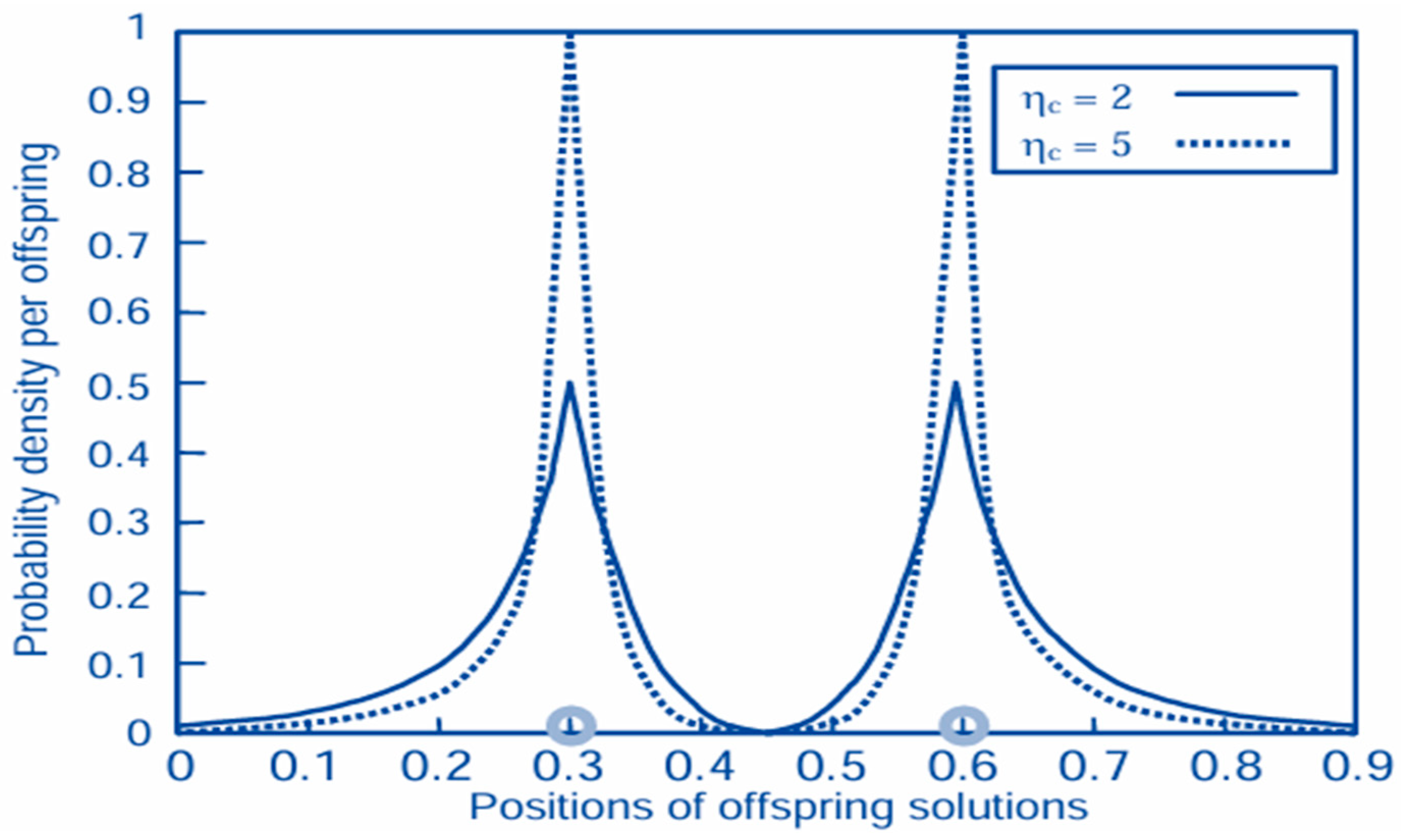
From GA, the Estimated Time of Arrival (ETA) value, or (ηc), in simulated binary crossover (SBX) controls the spread of offspring around their parents, with a greater value of η producing offspring closer to their parents and a smaller value allowing for more distant solutions to be selected, as shown in Figure 7. Large ηc tends to generate children closer to their parents, and small ηc allows the children to be farther from their parents.

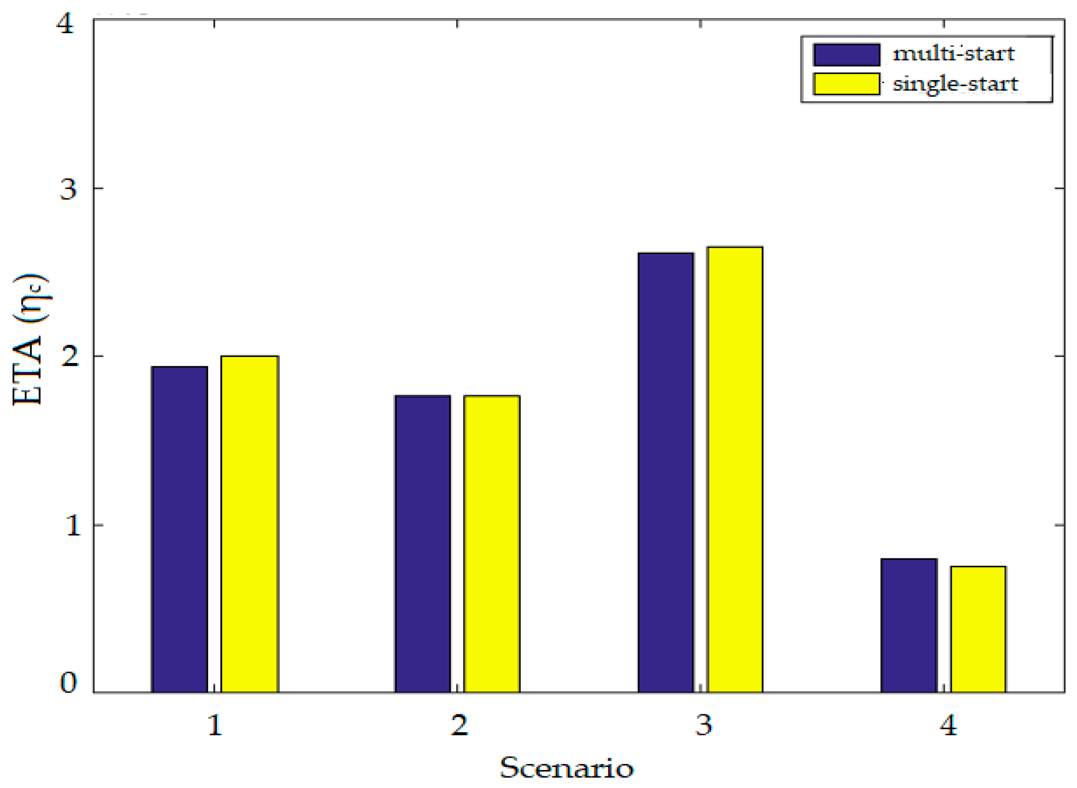
Following the execution of four scenarios for traffic optimization utilizing GA and LSTM networks, the resultant data are presented in Figure 8. This figure illustrates the ETA values achieved across the four traffic scenarios, encompassing two specific conditions: initiation from multiple points and initiation from a single point. The initial population for the genetic algorithm in this analysis was established at 50.

The analysis presented in Figure 8 indicates that the performance differential between the genetic algorithm utilizing multiple starting points and that employing a singular starting point is minimal. The observed performance of the algorithm without a multi-start approach in certain instances can be attributed to the presence of a single initial point combined with a more effective random number generator relative to the multi-start variant.

Considering the negligible variations in the ETA values, computational time emerges as the subsequent critical factor for examination. The insights gained from these four scenarios suggest that implementing a multi-start approach in genetic algorithms for optimization may be unwarranted, particularly given the importance of computational efficiency. It is noteworthy that extended simulation durations, coupled with an increased number of starting points for each iteration, could yield more pronounced performance disparities.

Table 3. Time value required for the proposed optimization solution with GA.

GA	Multi-Start Average Time [s]	Multi-Start Maximum Time [s]	Single-Start Average Time [s]	Single-Start Maximum Time [s]
Scenario 1	48.39	55.19	2.36	2.57
Scenario 2	66.19	73.83	3.05	3.81
Scenario 3	47.55	51.78	2.28	2.52
Scenario 4	47.71	50.07	2.37	3.98

presents the average and maximum computational times required for calculating the proposed optimization solutions using the genetic algorithm across the evaluated scenarios.

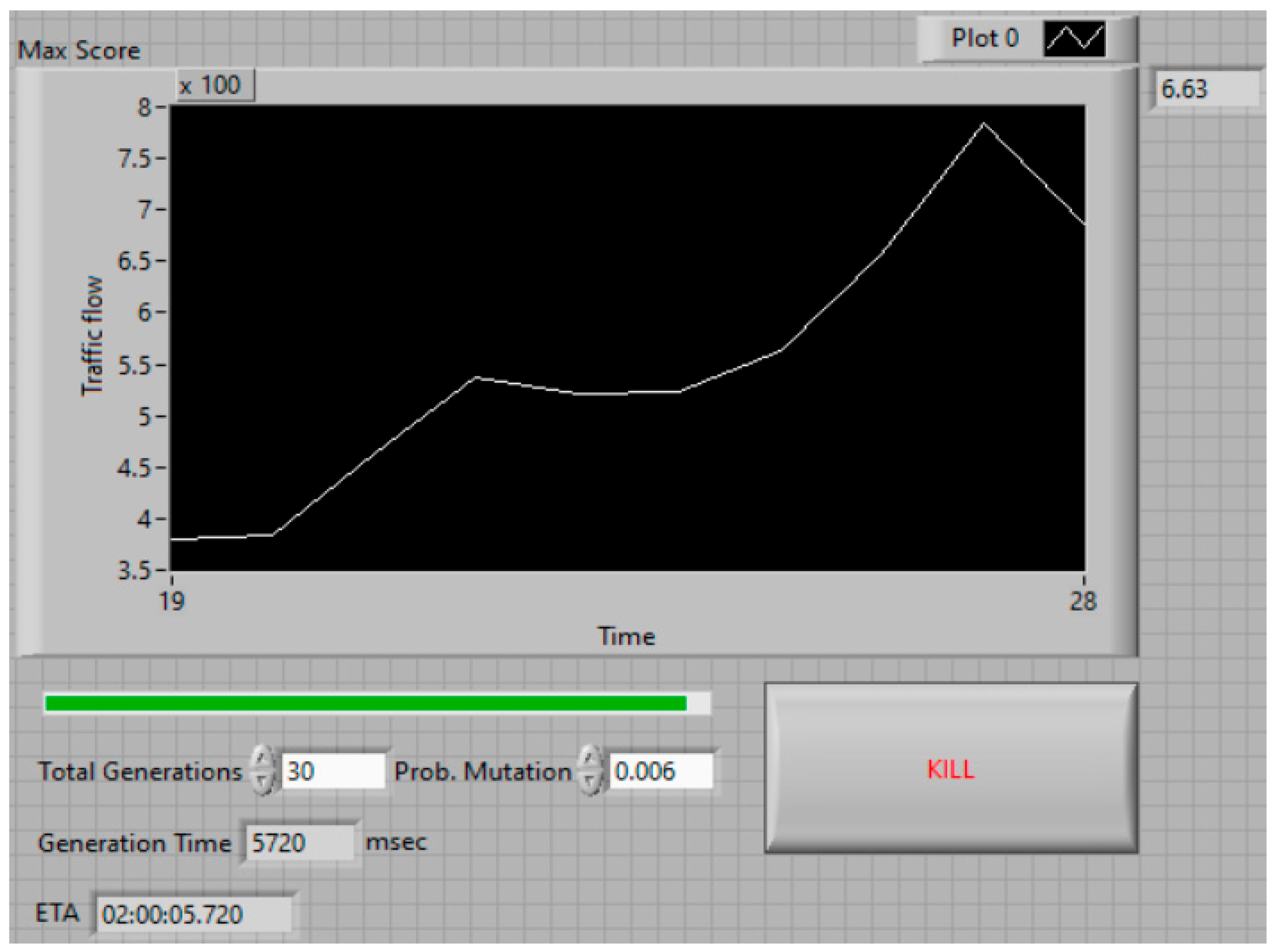
Figure 9 illustrates the software interface for the GA optimization algorithm based on the lines of code presented in Figure 5 and the results obtained for the ETA value and computation time in traffic optimization. The probability mutation parameter allows for adaptive adjustment, thereby improving the GA.

The adaptive mutation probability introduced in the proposed genetic optimization algorithm dynamically adjusts the mutation rate based on the population’s fitness. Typically, it increases for individuals with low fitness to maintain diversity and prevent premature convergence, while it decreases for individuals with high fitness to preserve good genetic combinations and promote convergence. This strategy employs a fitness-dependent formula, where a high mutation rate is applied when the individual’s fitness is poor, encouraging exploration, and a low mutation rate is used when the fitness is high, favoring exploitation.

4. Discussion

In the analysis of traffic flows and the pursuit of fluidization, a method utilizing the LSTM-GA was proposed and subsequently validated. This approach involved determining the optimal ETA value based on a probability mutation parameter through adaptive testing. The ETA value derived from this parameter allows for dynamic adjustments to the mutation rate, contingent upon the adaptability of the population.

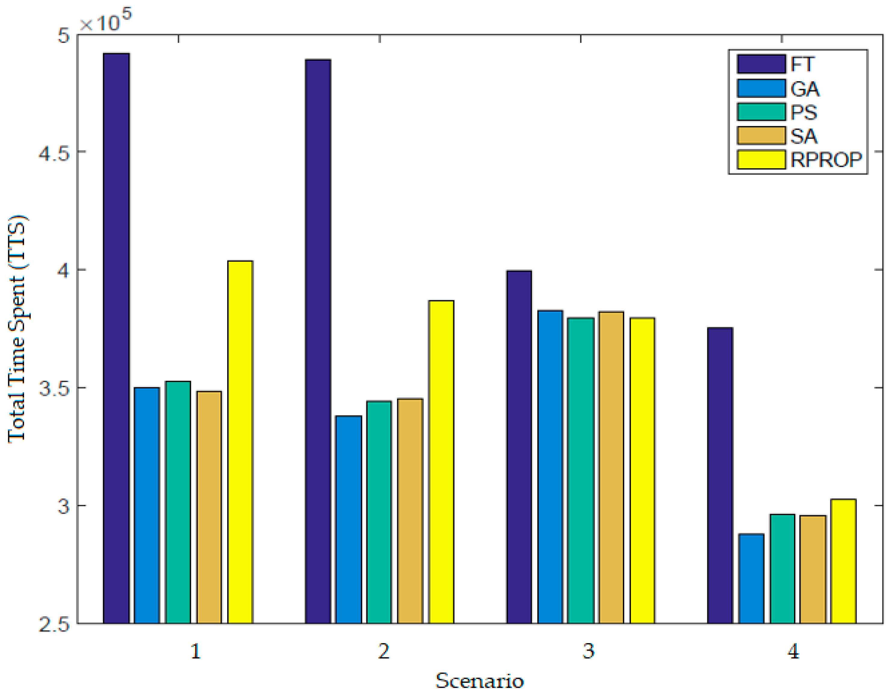
To underscore the efficacy of employing genetic algorithms for traffic optimization, a comparative analysis was conducted between the outcomes of the proposed LSTM-GA solution and those of other established algorithms in the literature. The results yielded by GA were compared with those of several optimization methods, specifically the fixed-time controller (FT), pattern search (PS), resilient backpropagation method (RPROP), and simulated annealing (SA). For comparison, we used the following algorithms: fixed-time controller (FT), pattern search (PS), resilient backpropagation method (RPROP), and simulated annealing (SA).

We chose these algorithms because the fixed-time traffic controller (FT) is a traffic algorithm that operates on a pre-established schedule, which does not change and depends on traffic light times. The pattern search algorithm (PS) is based on machine learning or clustering models to identify traffic patterns and optimize them. Resilient backpropagation method (RPROP) is an algorithm that can be used to train a neural network; it is similar to BP but is faster than training BP neural networks. Simulated annealing (SA) is a method for solving optimization problems without constraints or with limited constraints. The four algorithms mentioned were used in real-time traffic optimization applications.

The assessment of results was informed by prior studies, particularly those focusing on the methodologies of FT [32], PS [33], RPROP [34], and SA [35].

For the four test scenarios, for each of the algorithms chosen for comparison (FT, PS, RPROP, and SA), we considered the same starting points and calculation conditions.

Table 4. Results obtained for optimizing the four scenarios under multiple start conditions for 30 cycles.

TTS, ΔTTS (%) Multiple Start	FT	GA	SA	PS	RPROP
Scenario 1	4.92 41.7%	3.47 0%	3.46 −0.2%	3.52 1.6%	3.85 10.9%
Scenario 2	4.89 44.5%	3.38 0%	3.43 1.3%	3.45 1.9%	3.89 14.9%
Scenario 3	4.00 5.1%	3.81 0%	3.78 −0.6%	3.82 0.5%	3.88 1.9%
Scenario 4	3.75 29.4%	2.90 0%	2.94 1.6%	2.95 1.6%	2.94 1.4%

shows that the genetic algorithm has the best results for scenarios 2 and 4, and the SA algorithm has comparable results for scenarios 1 and 3.

Table 5. Results of the average time it took the algorithms to calculate the optimal solution for a single cycle.

TTS, ΔTTS (%) Multiple Start	FT	GA	SA	PS	RPROP
Scenario 1	0 −100%	48.39 0%	741.64 1432.5%	22.89 −52.7%	52.62 8.7%
Scenario 2	0 −100%	66.19 0%	766.39 1057.8%	26.45 −60.0%	57.94 −12.5%
Scenario 3	0 −100%	47.55 0%	744.58 1465.9%	11.19 −76.5%	77.00 61.9%
Scenario 4	0 −100%	47.71 0%	785.61 1546.7%	21.00 −56.0%	28.12 −41.1%

shows the average time it took to calculate the optimal solution for a single cycle. Since the fixed-time controller (FT) only implements a fixed ratio based on the cycle duration for each semaphore, it has no calculations, and we consider the time required to be zero. Pattern search (PS) appears to be the fastest algorithm, completing the calculations in less than half a minute in all scenarios, on average.

The genetic algorithm (GA) is in second place, with about a minute per cycle, as is the RPROP, although very different results are observed for RPROP. The performance of simulated annealing (SA) is poor in terms of computational time, even when the stopping criteria are reduced, taking more than an hour to complete. Overall, the genetic algorithm (GA) performs best in terms of cost function reduction, followed by simulated annealing (SA) and then pattern search (PS). Based on computational time, PS has outstanding performance, followed by GA and RPROP.

An evaluation of the data obtained in relation to the findings reported in the specialized literature led to the conclusions illustrated in Figure 10.

Figure 10 presents the comparative results for the four proposed traffic scenarios using the optimization algorithms (GA, FT, PS, RPROP, and SA), reported as total time spent (TTS), a key metric in traffic flow theory and intelligent transport systems (ITSs) that measures vehicle delay and congestion. In the four scenarios proposed in the article and used for comparison, the GA had the best results in terms of reducing TTS in the intersection.

The following conclusions are drawn from the comparative analysis:

-

The SA algorithm has minimum and maximum performance values depending on the tested scenario.

-

The SA algorithm’s performance is almost equal to that of the PS algorithm but weaker than that of the GA.

-

The RPROP algorithm’s performance is influenced by the degree of traffic congestion. If the degree of congestion is high, the RPROP algorithm’s performance is low compared to the GA.

-

The FT algorithm has the lowest results compared to the other optimization algorithms analyzed.

The present research was conducted under controlled simulation conditions, which, although valuable for testing algorithmic performance, may not fully capture the variability and complexity of real-world traffic environments. The study was restricted to a simplified urban network with three intersections and a limited set of scenarios. Furthermore, the optimization process relied on average traffic flow assumptions and did not consider external factors such as weather, road incidents, or heterogeneous driver behaviors, which could significantly influence prediction accuracy and system adaptability.

Future work should focus on validating the GA-LSTM framework with large-scale, real-time traffic data collected from diverse urban settings. The results obtained from testing the GA-LSTM on real traffic data from Bucharest were encouraging, so the main research direction in the future will be to test the algorithm in real traffic conditions with data obtained from sensors. The real-time testing will be carried out in the Traffic Management Center in Bucharest.

Expanding the model to multi-intersection networks and incorporating connected vehicle and Internet of Things (IoT) data streams would enhance its robustness and applicability. Additionally, integrating adaptive mechanisms, such as dynamic parameter tuning or reinforcement learning strategies, could enhance scalability and responsiveness in rapidly changing traffic conditions.

The process of microsimulation of road traffic can be used to study the effects of traffic management schemes, traffic light control methods, or public transport prioritization systems. The models resulting from the simulation of different traffic scenarios help to accurately assess the effects of heavy vehicle traffic or congestion. With the help of this data (vehicle type, speed, acceleration, its position in each second, etc.), the effects of different traffic scenarios can be tracked, and situations in which traffic safety is compromised by disruptive factors (weather, road incidents, and driver behavior) can be assessed. The disadvantages of using microsimulation models in assessing traffic compromised by disturbance factors are as follows: the stochastic nature of microsimulation requires multiple model runs, which are time-consuming; the road networks must be defined with more precision than is typically required; the stability of the models may depend on the selection of a certain time step value that influences the traffic modeling under disturbance conditions; and a wide range of input parameters may pose potential challenges. In future research on the model used in the article, we will also introduce traffic models compromised by disturbance factors to test the proposed algorithm under these conditions.

These directions would contribute to the development of intelligent, resilient, and sustainable urban mobility systems.

5. Conclusions

This study proposed an optimization model for urban traffic smoothing based on the integration of a GA with a recurrent neural network of the LSTM type. The hybrid GA-LSTM framework demonstrated the capacity to capture traffic dynamics while simultaneously optimizing key parameters through evolutionary computation. The results indicated that the combined approach achieved superior prediction accuracy and improved the efficiency of traffic flow control compared to conventional strategies.

The comparative analysis performed across four simulated traffic scenarios confirmed that the GA-LSTM approach consistently reduced the total time spent at intersections. When benchmarked against established optimization methods (FT, PS, RPROP, and SA), the proposed model delivered the most favorable results in terms of congestion mitigation and travel time reduction. These findings underscore the importance of integrating data-driven learning with heuristic optimization in intelligent transportation systems.

Beyond the immediate improvements demonstrated in simulation, the GA-LSTM framework provides a scalable foundation for future research. Further validation using large-scale, real-world traffic data will be essential to confirm its robustness under diverse conditions. In addition, extensions of the model could include adaptive mechanisms for real-time deployment, integration with connected vehicle data, and testing in multi-intersection or city-wide networks. Such directions may strengthen the contribution of the proposed methodology to the development of sustainable and intelligent urban mobility solutions.