Drone–Rider Joint Delivery Routing with Arc Obstacle Avoidance

Abstract

Drone delivery has gained significant traction in e-commerce, particularly for parcel and food delivery. However, existing systems face challenges such as limited delivery range, low efficiency, high costs, and suboptimal customer satisfaction. This paper proposes a novel drone–rider joint delivery model incorporating an Arc Obstacle Avoidance (AOA) strategy to address these issues in complex urban environments. We formulate a multi-objective optimization model aimed at minimizing delivery costs and maximizing customer satisfaction, solved by a Logistic-Logarithmic Dung Beetle Optimization algorithm (LLDBO). Using a modified Solomon dataset and real-world urban simulations in Shenzhen, our experiments demonstrate that the proposed model achieves a 15.3% reduction in delivery costs and a 27.1% increase in delivery efficiency compared to traditional rider-only delivery. Furthermore, customer satisfaction, measured by the on-time delivery rate, shows a 12.4% improvement (from 83.1% to 95.5%) over the rider-only baseline. The AOA strategy also extends the effective delivery range by up to 22.5% compared to conventional linear obstacle avoidance approaches, as measured by the maximum service radius achievable while maintaining 95% on-time delivery performance. These findings validate the practicality and scalability of the proposed approach for real-world last-mile logistics.

1. Introduction

The rapid growth of e-commerce has fundamentally transformed consumer behavior and expectations, particularly in the food delivery sector. Takeout delivery has evolved into a crucial component of modern digital commerce ecosystems, seamlessly integrating online transaction platforms with physical distribution services [1]. This integration has created new paradigms in retail logistics, where timely delivery has become as important as product quality itself. However, despite significant technological advancements, the industry continues to grapple with fundamental operational challenges including geographical delivery limitations, efficiency constraints, escalating costs, and inconsistent customer satisfaction levels [2]. These challenges become particularly pronounced in densely populated urban environments where traffic congestion and complex logistics networks further complicate last-mile delivery operations.

The emergence of unmanned aerial vehicle technology offers promising solutions to these persistent challenges. Major global logistics providers including Amazon have initiated commercial drone delivery programs, demonstrating the substantial potential of aerial vehicles to overcome traditional road-dependent constraints and significantly improve delivery efficiency [3]. The theoretical foundations for these systems were established in early research on drone-assisted parcel delivery, notably through formulations such as the Flying Sidekick Traveling Salesman Problem (FSTSP) which provided mathematical frameworks for integrating drones into existing delivery networks [4]. Subsequent research has expanded these concepts to include more complex operational scenarios, including two-echelon vehicle routing problems that systematically optimize the coordination between ground vehicles and drones in last-mile delivery contexts [5].

However, the practical implementation of drone-based delivery systems in complex urban environments faces two critical technical challenges that existing literature has yet to adequately address. First, the development of effective navigation systems capable of safely avoiding urban obstacles while maintaining delivery efficiency remains a significant research gap [6]. Current obstacle avoidance algorithms often rely on simplified environmental models that fail to capture the complexity of real-world urban landscapes. Second, operational coordination between drones and traditional delivery vehicles presents substantial logistical challenges, particularly in optimizing handover processes and minimizing idle times [7]. Existing coordination models based on synchronized arrivals at transfer points create scheduling bottlenecks that reduce overall system efficiency, as identified in extended vehicle routing problems with drones [8].

This paper proposes a comprehensive framework for drone–rider joint delivery that introduces several innovative solutions to address these limitations. Our approach incorporates a novel arc obstacle avoidance (AOA) strategy that enables drones to navigate around urban obstacles along optimized curved flight paths, significantly reducing detour distances compared to conventional methods. Additionally, we establish a network of strategically positioned drone stations equipped with intelligent takeout lockers, creating asynchronous transfer points that eliminate the requirement for precise synchronization between drones and riders. This architectural innovation substantially reduces waiting times and increases system flexibility.

To solve the complex routing optimization problems inherent in our proposed system, we have enhanced the established Dung Beetle Optimization algorithm [9] through the incorporation of chaotic mapping techniques for population initialization and logarithmic-based dynamic allocation mechanisms for population proportion adjustment. These modifications result in our improved LLDBO algorithm, which demonstrates superior performance in handling the multi-objective optimization challenges presented by joint delivery systems.

The main contributions of this research are threefold: (1) the development of a novel arc obstacle avoidance strategy specifically designed for drone navigation in complex urban environments; (2) the creation of an enhanced drone–rider coordination framework utilizing dedicated transfer stations to optimize operational efficiency; and (3) the introduction of an improved metaheuristic optimization algorithm (LLDBO) for solving complex routing problems in multi-modal delivery systems.

The paper is structured as follows: Section 2 reviews the relevant literature, Section 3 outlines the problem and introduces the model, Section 4 describes the algorithm and its improvements, Section 5 presents simulation experiments and analyzes the results, and Section 6 summarizes the findings, highlighting contributions and potential future research directions.

2. Literature Review

This section provides a comprehensive review of the relevant literature, organized into four main subsections. The review begins with an examination of drone delivery route optimization studies, followed by an analysis of customer satisfaction and time window considerations in last-mile delivery. Subsequently, research on drone obstacle avoidance and urban operations is discussed. Finally, the research gap and our contribution are clearly delineated.

2.1. Optimization Study of Drone Delivery Routes

Research on drone route optimization primarily focuses on two directions: standalone drone delivery and joint drone–truck delivery. Drone technology continues to evolve, and research in this field is expanding. The integration of drones with various transportation modes has emerged as a particularly promising research direction [10].

2.1.1. Standalone Drone Delivery Optimization

A significant body of work focuses on optimizing routes for drones operating independently. Early foundational work by Murray and Chu [4] introduced the Flying Sidekick Traveling Salesman Problem (FSTSP), a seminal model that has inspired numerous variants. Dorling et al. [11] further refined this model by considering multiple drones per truck, highlighting the trade-offs between launch energy and delivery coverage.

Recent advances have incorporated more complex real-world constraints using sophisticated metaheuristics, as summarized in Table 1. For instance, Zhang et al. [12] developed a multi-mode collaborative multi-objective particle swarm optimization algorithm (MCMOPSO-RL) to handle complex routing scenarios. Similarly, Chowdhury and De [13] proposed a Reverse Glowworm Swarm Optimization Algorithm (RGSO) for 3D drone path planning in dynamic environments, addressing the need for altitude-aware routing. Huang et al. [14] contributed an adaptive cylinder vector particle swarm optimization integrated with differential evolution, enhancing solution quality for complex drone routing problems.

Table 1. Comparison of Standalone Drone Delivery Optimization Methods.

Study	Key Contribution	Optimization Method	Main Limitations
[4]	Introduced FSTSP model	Mixed-integer programming	Single drone per truck assumption
[11]	Multiple drones per truck	Heuristic algorithms	Simplified energy consumption model
[12]	MCMOPSO-RL algorithm	Multi-objective PSO	Limited real-world validation
[15]	Green multi-package delivery	Efficient metaheuristics	Limited to standalone drone operations
[13]	3D path planning in dynamic environments	Reverse Glowworm Swarm Optimization	High computational complexity
[14]	Adaptive cylinder vector PSO with DE	Hybrid metaheuristic	Neglects urban obstacle constraints

While these studies advance algorithmic sophistication, they often assume unconstrained airspace, neglecting the critical impact of urban obstacles on route feasibility and cost.

2.1.2. Optimization of Joint Drone and Truck Delivery Routes

Collaborative systems leverage the synergy between drones’ aerial agility and vehicles’ high capacity and range. The Truck–Drone Routing Problem (TDRP) is a well-established paradigm in this domain. Salama and Srinivas [16] explored a tandem variant where trucks can park at non-customer locations to launch and recover drones, significantly increasing operational flexibility. Lu et al. [17] investigated a bi-objective green vehicle routing problem incorporating heterogeneous regular vehicles and occasional drivers in joint delivery scenarios.

Beyond package delivery, this paradigm is highly relevant to time-sensitive applications. Peng et al. [18] investigated a truck–drone collaborative routing problem with dynamic emergency response in humanitarian logistics, emphasizing robustness. For a comprehensive review of modeling approaches and challenges in this field, readers are referred to the survey by Otto et al. [2]. The key characteristics and limitations of these joint delivery approaches are systematically compared in Table 2. Notably, Lu et al. [19] further advanced this field by developing routing optimization for takeout delivery involving drones, occasional drivers, and riders, addressing the specific challenges of food delivery logistics.

Table 2. Comparison of Joint Drone–Truck Delivery Optimization Methods.

Study	Application Context	Coordination Mechanism	Main Limitations
[19]	Takeout delivery	Drones, occasional drivers, riders	Urban obstacle constraints not considered
[17]	Green vehicle routing	Heterogeneous vehicles, occasional drivers	Focus on environmental aspects only
[16]	Parcel delivery	Flexible parking locations	Simplified handover process
[18]	Humanitarian logistics	Dynamic emergency response	Limited urban environment focus
[2]	Comprehensive survey	Classification of models	No original algorithm proposed

A common limitation across these studies is the treatment of the handover process between the drone and the ground unit as instantaneous and cost-free, an assumption that does not hold in practical urban settings with coordination delays.

2.2. Customer Satisfaction and Time Windows in Last-Mile Delivery

This subsection examines how customer satisfaction and time window constraints have been addressed in last-mile delivery research. In the context of e-commerce and food delivery, customer satisfaction is intrinsically linked to on-time delivery, making time windows a critical constraint.

Research in this area often models satisfaction through penalty functions for early or late arrivals. [20] formulated a dynamic vehicle routing problem that explicitly incorporated customer satisfaction metrics into the objective function. More recently, [21] analyzed the route efficiency implications of combining first-mile pickups and last-mile deliveries under strict time windows, highlighting the operational complexities in dense urban networks.

The time window vehicle routing problem (VRPTW) has been extensively studied. [22] proposed a new exact method based on an extended A* algorithm for the time-dependent TSP with time windows, pushing the boundaries of optimal solution finding for medium-sized instances. For drone-specific applications, [23] tackled the vehicle routing problem with drones considering time windows, demonstrating the potential for improved service levels.

However, these studies typically employ linear penalty functions for time window violations, which may not accurately capture the non-linear nature of customer dissatisfaction—an issue this paper seeks to address.

2.3. Drone Obstacle Avoidance and Urban Operations

This subsection reviews strategies for enabling safe drone operations in urban environments, covering both strategic no-fly zone avoidance and tactical real-time path planning approaches.

Operating drones in urban environments necessitates robust obstacle avoidance strategies. Current research can be categorized into strategic no-fly zone avoidance and tactical real-time path planning. [24] incorporated static no-fly zones and payload-energy dependency into a truck–drone hybrid routing model, acknowledging the spatial constraints of urban airspace. [25] contributed a methodology for generating ground risk maps for unmanned aircraft in urban environments, which can be used to define risk-aware no-fly zones.

On the tactical level, algorithms for real-time obstacle detection and avoidance are crucial. [26] proposed a path planning algorithm using sensor-based real-time obstacle mapping, suitable for dynamic environments. [27] established an expansion model for electric vehicle charging station site selection based on GIS-FAHP-MABAC methodology. Recent studies on last-mile delivery with drones and vehicles [28] further highlight the operational challenges in integrated ground-aerial systems. However, most routing-level studies treat obstacle avoidance as a binary constraint (avoid or not) rather than a continuous optimization problem where the cost of avoidance (e.g., detour distance, energy) is minimized. Furthermore, the assumption of perfect communication and the absence of hardware failures, as seen in many models, presents a significant gap between theoretical models and real-world deployability.

2.4. Research Gap and Our Contribution

Based on the comprehensive literature review, this subsection clearly identifies the research gaps and outlines the specific contributions of this work.

As evidenced by the literature, substantial progress has been made in drone routing, collaboration with ground vehicles, and obstacle avoidance in isolation. However, a critical gap exists in the integration of these aspects into a unified framework for last-mile food delivery. Existing models often overlook: (1) the operational intricacies and costs of handovers between drones and riders in a urban setting; (2) the optimization of the avoidance maneuver itself (e.g., arc path optimality) within routing algorithms, rather than simply avoiding zones; and (3) the impact of real-world constraints such as non-linear customer dissatisfaction, battery degradation, and dynamic obstacles. While hybrid optimization approaches have been explored for vehicle-drone systems [29], they often overlook the operational intricacies of handovers in dense urban settings.

This paper bridges these gaps by proposing a holistic drone–rider joint delivery model that incorporates a novel Arc Obstacle Avoidance (AOA) strategy. Unlike previous work, our model explicitly minimizes the cost of avoidance detours, employs a non-linear penalty for time window violations to better model customer satisfaction, and introduces a more efficient metaheuristic (LLDBO) to solve the resulting complex problem. By doing so, we provide a more realistic and scalable solution for last-mile logistics in complex urban environments. Our proposed drone–rider joint delivery mode builds upon our prior work on order distribution optimization and shared logistics models for meal delivery [1,19], but significantly extends it by integrating a novel obstacle avoidance strategy and a more efficient metaheuristic solver.

3. Problem Description and Modeling

This section presents the formal problem description and mathematical modeling of the proposed drone–rider joint delivery system. The section begins with an overview of the problem context and operational framework, followed by a detailed description of the novel Arc Obstacle Avoidance strategy.

3.1. Description of the Problem

The rapid development of drone delivery services has created new opportunities for enhancing urban logistics networks [4]. Building upon established collaborative delivery concepts [5,7], this study addresses the critical challenge of optimizing food delivery in complex urban environments through a novel drone–rider joint delivery system, with the operational workflow illustrated in Figure 1.

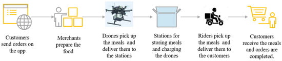
Figure 1. Flowchart of drone–rider joint delivery mode.

The proposed operational framework extends existing collaborative models through several key innovations. Merchant aggregation points serve as meal distribution centers, functioning as origination points for drone operations. Unlike traditional approaches that require direct synchronization between drones and riders [8], our system introduces strategically located drone stations that enable asynchronous operations, thereby eliminating coordination bottlenecks and reducing waiting times.

Riders operate within predefined service areas determined by Euclidean distance constraints, consistent with established practices in last-mile delivery optimization [10]. The integration of dedicated drone stations as intermediate transfer points represents a significant departure from conventional models, allowing for decoupled operations that enhance system flexibility and reliability.

3.2. Arc Obstacle Avoidance (AOA)

Urban drone operations must navigate various no-fly zones, including tall structures and restricted airspace [10]. While existing research has primarily treated obstacle avoidance as a binary constraint, our approach optimizes the avoidance path itself to minimize detour costs. The proposed Arc Obstacle Avoidance (AOA) strategy generates optimized curved trajectories that reduce total travel distance compared to conventional linear avoidance methods.

When a drone’s planned path intersects with a no-fly zone, the system initiates an avoidance procedure that constructs multiple candidate paths using geometric transformations and selects the optimal trajectory based on minimal distance criteria, as illustrated in Figure 2. The core innovation lies in the simultaneous evaluation of circular and elliptical arcs relative to the obstacle geometry, ensuring safe clearance while minimizing travel distance.

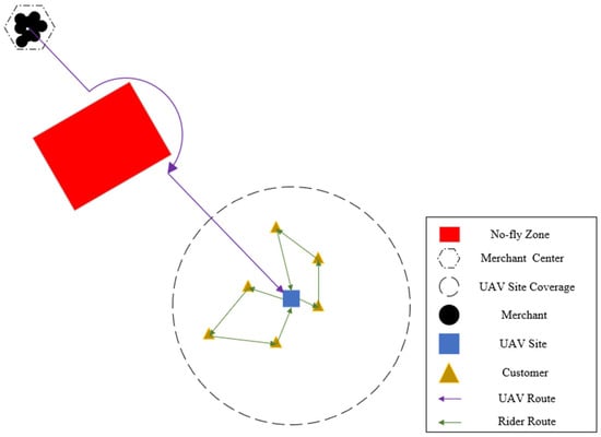
Figure 2. Schematic diagram of arc obstacle avoidance in the no-fly zone of drones.

This approach fundamentally differs from existing methods by treating obstacle avoidance as a continuous optimization problem rather than a simple constraint satisfaction task. By focusing on practical approximation methods that balance computational efficiency with path optimality, our AOA strategy achieves significantly better performance than conventional approaches while remaining computationally feasible for real-time operations.

3.3. Formulation of Hypotheses

(1) Riders picking up and delivering food have a certain service time, and the service time is fixed.

(2) There is a one-to-one correspondence between merchant points and customer points. Multiple customers who place orders with the same takeout merchant are assigned to multiple merchant points with the same coordinates. If a customer places orders with multiple merchants, multiple merchant points will be assigned to multiple customer points with the same coordinates.

(3) There is no limit to the number of drones that can be accommodated at a drone site.

(4) Riders travel at a constant speed.

(5) Accidents, weather, and other unforeseen circumstances are not considered in the delivery.

3.4. Modeling

3.4.1. Model Parameters

The model parameters are shown in Table 3.

Table 3. Description of model symbols.

Index	Parameters	Parameter Description
parameter	$C$	Customer Point Gathering $C=\left\{c_1,c_2,\dots ,c_n\right\}$
	$P$	A collection of alternative drone sites $P=\left\{p_1,p_2,\dots ,p_n\right\}$
	$U$	Enabling a collection of drone sites, $U=\left\{u_1,u_2,\dots ,u_n\right\}$ $U\in P$
	$S$	A collection of drone sites at merchant gathering points $S=\left\{s_1,s_2,\dots ,s_n\right\}$
	$H_1$	Enabling a collection of drone sites and merchant locations $H_1=U\cup S$
	$H_2$	Enabling a collection of drone sites and customer points $H_2=U\cup C$
	$K$	A collection of riders $K=\left\{k_1,k_2,\dots ,k_n\right\}$
	$D$	A collection of drones $D=\left\{d_1,d_2,\dots ,d_n\right\}$
	$a_1$	Fixed cost of using a single drone for drone pickups
	$a_2$	Fixed cost of individual rider deliveries when riders deliver meals
	$b_1$	Drone straight-line flight cost per unit distance delivered
	$b_2$	Rider delivery cost per unit distance
	$b_3$	Drone Arc Flight Unit Distance Distribution Costs
	$Q_1$	Capacity cap when picking up food by drone
	$Q_2$	Delivery capacity cap for riders delivering food
	$F{D}_S$	Fixed costs for a drone site $s$ established at a merchant aggregation point, the $s\in S$
	$C{D}_S$	Drone Sites at Merchant Gathering Points $s$ capacity. $s\in S$
	$F{D}_u$	Fixed costs of establishing a transit drone site $u$. $u\in U$
	$C{D}_u$	Capacity of the transit drone site $u$. $u\in U$
	$n_{ij}$	The Euclidean distance between the point $i$ and the point $j$, the $i,j\in U\cup S\cup G$
	$n_{ij}^d$	The Euclidean distance of the drone from the point $i$ to the point $j$, the $i,j\in U\cup S\cup G$
	$n_{ij}^k$	The distance the rider traveled from point $i$ to point $j$ in Manhattan. $i,j\in C\cup U$
	$r_{ij}$	The distance in arc of the drone from the point $i$ to the point $j$, the $i,j\in G$
	$T_{ck}$	Time for rider to reach customer point $c$$, c\in C, k\in K$
	$R$	The set of circles with the longest diagonal of the no-fly zone as their diameter. $R=\left\{r_1,r_2,\dots ,r_n\right\}$
	$G$	The intersection of the flight route of the drone from the point $i$ to the point $j$ with the set $R$. $i,j\in H_1$
	$\theta$	The angle of the center of the circle $r\in R$, corresponding to the line between the point $i$ and the point $j$ on the circle. $r$ $i,j\in G$
	$O$	Gathering in the no-fly zone $O=\left\{o_1,o_2,\dots ,o_n\right\}$
	$V_k$	Rider speed
	$V_s$	Drone linear flight speed
	$V_r$	Drone arc flight speed
	$s$	Rider service hours
	$p_1$	Time penalty costs for early arrival
	$p_2$	Time penalty costs for late arrival
	$E{E}_c$	Early to Hard Time Window for Rider Deliveries
	$E_c$	Early to soft time window for rider deliveries
	$L{L}_c$	Late arrival hard time window for rider deliveries
	$L_c$	Late arrival soft time window for rider deliveries
	$m_t$	Weight of the drone
	$m_b$	Weight of drone batteries
	$m_l$	Weight of drone-delivered meals
	$g$	Gravitational acceleration
	$\eta$	Energy conversion efficiency
	$f$	Energy consumption per unit distance traveled by a drone at a constant speed
	$f(m_l)$	Energy consumption per unit distance flown at constant speed by a drone in the case of meal delivery
	${\vartheta }_v$	Ratio of flight departure resistance, usually as a function of velocity
	$d$	Unit distance
Decision variables	$\alpha$	Parameters of the energy consumption formula
	$\beta$	Parameters of the energy consumption formula
	$x_{ij}$	If the drone goes from point $i$ to point $j$, then $x_{ij}=1$; otherwise, $x_{ij}=0$ $i,j\in H_1$
	$y_{lm}$	If the rider goes from point $l$ to point $m$, then $y_{lm}=1$; otherwise, $y_{lm}=0$ $l,m\in H_2$
	$z_s$	If the merchant point $s$ has meals to be delivered, then $z_s=1$; otherwise, $z_s=0$ $s\in S$
	$u_p$	If the drone site $p$ is selected as a staging area, then $u_p=1$; otherwise, $u_p=0$ $p\in P$
	$l_{sp}$	If the drone site $p$ is assigned to the merchant aggregation site $s$, then $l_{sp}=1$; otherwise, $l_{sp}=0$ $, s\in S, p\in P$
	$q_{cp}$	If the drone site $p$ is assigned to the customer site $c$, then $q_{cp}=1$; otherwise, $q_{cp}=0$$, c\in C, p\in P$
	$h_o$	If the drone’s flight route coincides with the no-fly zone $o$, then $h_o=1$; otherwise, $h_o=0$ $o\in O$

3.4.2. Objective Function

$F$ indicates that the total cost of delivery is minimized.

$F_1$ From left to right, the cost of drone pickup and transportation, the construction cost of drone stations at merchant gathering points, the fixed cost of drone pickup, the transportation cost of rider delivery, the cost of opening a drone staging site, the fixed cost of rider delivery, and the cost of drone avoidance and detour.

$F_2$ Indicates the cost of time penalties.

$$\min F=F_1+\lambda F_2$$

(1)

$$\begin{array}{cc}{F}_1=& {\displaystyle \sum _{i\in H_1}{\displaystyle \sum _{j\in H_1}{b}_1{n}_{ij}^d{x}_{ij}}}+{\displaystyle \sum _{s\in S}F{D}_s{z}_s}+{\displaystyle \sum _{s\in S}{\displaystyle \sum _{u\in U}{a}_1}}{x}_{su}+{\displaystyle \sum _{l\in H_2}{\displaystyle \sum _{m\in H_2}{b}_2{n}_{lm}^k}}{y}_{lm}+\\ & {\displaystyle \sum _{u\in U}F{D}_u}{u}_u+{\displaystyle \sum _{u\in U}{\displaystyle \sum _{c\in C}{a}_2}}{y}_{cu}+{\displaystyle \sum _{l\in G}{\displaystyle \sum _{m\in G}{\displaystyle \sum _{o\in O}{b}_3{r}_{lm}}{h}_o}}-{\displaystyle \sum _{l\in G}{\displaystyle \sum _{m\in G}{\displaystyle \sum _{o\in O}{b}_2}{n}_{lm}{h}_o}}\end{array}$$

(2)

$$F_2=p(T_{ck})=\left\{\begin{array}{l}{p}_1(E_c-T_{ck}),E{E}_C<T_{ck}<E_c\\ 0,E_c<T_{ck}<L_c\\ p_2(T_{ck}-L_c),L_c<T_{ck}<L{L}_c\\ 1000,T_{ck}<E{E}_c\mathrm{or}{T}_{ck}>L{L}_c\end{array}\right.$$

(3)

The drone load is $m_l$ and the horizontal flight energy consumption equation:

$$f(m_l)={\displaystyle \frac{(m_t+m_b+m_l)g}{3600{\vartheta }_v\eta }}d$$

(4)

With a drone load of $m_l$, it rises to altitude at a certain speed and then descends to the ground at the same speed, with air resistance approximately canceling out and the energy consumption equation:

$$f(m_l)={\displaystyle \frac{2(m_t+m_b+m_l)g}{3600{\vartheta }_v\eta }}d$$

(5)

$r_{ij}$ denotes the obstacle avoidance bypass distance of the drone, calculated by the equation $r_{ij}={\displaystyle \frac{\theta \pi R}{360}}$.

Equation (6) stipulates that each transit drone site must be visited exactly once, thereby ensuring complete coverage of all designated drone hubs in the routing plan.

Equation (7) ensures that open drone transit sites are assigned exclusively to drone stations located at merchant aggregation points where meal deliveries originate, linking drone operations directly to order sources.

Equation (8) specifies that each merchant aggregation site is allocated to only one drone transit site, preventing redundant assignments and maintaining operational clarity.

Equation (9) guarantees flow conservation by ensuring that the number of entry arcs equals the number of exit arcs at each node within the drone food pickup process, thereby maintaining route continuity.

Equation (10) similarly enforces flow balance for each node in the rider delivery process, ensuring that riders’ routes remain consistent and uninterrupted.

Equation (11) serves to eliminate sub-tours in the drone pickup route, thereby enforcing the formation of a single, coherent tour.

Equation (12) functions analogously to eliminate sub-tours within the rider delivery route, ensuring valid and efficient rider paths.

Equations (13)–(15) collectively prevent scenarios in which the starting and ending drone sites differ during the first level of the delivery process, thus enforcing route consistency at the initial stage.

Equation (16) imposes the condition that each customer must be served exactly once, which safeguards against both missed and duplicate deliveries.

Equation (17) requires that every customer is assigned to a specific drone transit site, thereby integrating customer locations into the drone network.

Equations (18)–(20) block situations where the starting and ending drone sites are not the same during the secondary delivery phase, ensuring route coherence in later operations.

Equation (21) defines capacity constraints for the drone delivery process, limiting the load that drones can carry.

Finally, Equation (22) specifies capacity constraints applicable to the rider delivery process, controlling the maximum delivery load per rider.

s.t.

$${\displaystyle \sum _{j\in H_1}{x}_{jp}}=u_p;\forall p\in P$$

(6)

$${\displaystyle \sum _{u\in U}{l}_{su}}\le \left|P\right|z_s;\forall s\in S$$

(7)

$${\displaystyle \sum _{u\in U}{l}_{su}}=1;\forall s\in S$$

(8)

$${\displaystyle \sum _{j\in H_1}{x}_{ij}}={\displaystyle \sum _{j\in H_1}{x}_{ji}};\forall i\in H_1$$

(9)

$${\displaystyle \sum _{m\in H_2}{y}_{lm}}={\displaystyle \sum _{m\in H_2}{y}_{ml}};\forall l\in H_2$$

(10)

$${\displaystyle \sum _{i\in H_1}{\displaystyle \sum _{j\in H_1}{x}_{ij}}}=\left|S\right|-1;2\le \left|S\right|\le N-1$$

(11)

$${\displaystyle \sum _{l\in H_2}{\displaystyle \sum _{m\in H_2}{y}_{lm}}}=\left|S\right|-1;2\le \left|S\right|\le N-1$$

(12)

$$x_{su}\le l_{su};\forall s\in S,\forall u\in U$$

(13)

$$x_{us}\le l_{su};\forall s\in S,\forall u\in U$$

(14)

$$x_{iu}+l_{is}+{\displaystyle \sum _{b\in S,b\ne s}{l}_{pb}}\le 2;\forall i,u\in U,i\ne u,\forall s\in S$$

(15)

$${\displaystyle \sum _{m\in H_2}{y}_{ml}}=1;\forall l\in C$$

(16)

$${\displaystyle \sum _{u\in U}{q}_{cu}}=1;\forall c\in C$$

(17)

$$y_{uc}\le q_{uc};\forall c\in C,\forall u\in U$$

(18)

$$y_{cu}\le q_{uc};\forall c\in C,\forall u\in U$$

(19)

$$y_{lc}+q_{lu}+{\displaystyle \sum _{e\in u,e\ne u}{q}_{ce}}\le 2;\forall l,c\in C,l\ne c,\forall u\in U$$

(20)

$${\displaystyle \sum _{s\in S}{\displaystyle \sum _{u\in U}{x}_{su}}}{g}_u\le Q_1$$

(21)

$${\displaystyle \sum _{c\in C}{\displaystyle \sum _{h\in H_2}{y}_{ch}}}{g}_c\le Q_2$$

(22)

4. Algorithm Design

The Dung Beetle Optimization (DBO) algorithm, proposed by Xue and Shen [9], has demonstrated notable efficacy in solving complex optimization problems due to its unique biological inspiration and balanced exploration-exploitation dynamics. Compared to other swarm intelligence algorithms such as Particle Swarm Optimization (PSO) and Genetic Algorithms (GA), DBO exhibits superior performance in avoiding premature convergence and maintaining population diversity, as validated in benchmark optimization tests [9]. These characteristics make DBO particularly suitable for the complex, multi-modal optimization landscape of drone-rider joint delivery routing problems.

Despite its strengths, the traditional DBO algorithm faces challenges in slow convergence speed and susceptibility to local optima in high-dimensional problems, limitations that are also observed in other population-based algorithms [30]. To address these issues while preserving the fundamental advantages of the DBO framework, this paper proposes an improved Logistic-Logarithmic Dung Beetle Optimization algorithm (LLDBO).

The novelty of our approach lies in two key modifications to the original DBO algorithm:

(1) Logistic Chaotic Mapping for Population Initialization: Building upon established chaotic optimization techniques [31], we employ Logistic chaotic mapping to generate the initial population. This enhancement ensures greater population diversity during the initialization phase, facilitating more comprehensive exploration of the solution space, as demonstrated in previous studies where chaotic maps have significantly improved optimization algorithm performance.

(2) Logarithmic Dynamic Population Allocation: Unlike the fixed population proportions in traditional DBO [9], we introduce a logarithmic function to dynamically adjust the proportions of different dung beetle roles (ball-rolling, breeding, small dung beetles, and thieves) throughout the optimization process. This innovation allows the algorithm to automatically balance global exploration and local exploitation as iterations progress, addressing dynamic coordination challenges similar to those encountered in flying warehouse systems [32] and joint delivery models [33].

Recent advances in hybrid optimization approaches [34] and deep reinforcement learning [35] have shown significant promise for multi-drone routing optimization, while coordinated charging strategies [36] further highlight the critical importance of efficient resource management in logistics systems. However, these advanced approaches often require extensive computational resources. It is important to note that our improvements specifically target the initialization and population management mechanisms, while preserving the core search operations of the original DBO algorithm, including ball-rolling behavior, breeding strategies, and stealing activities as defined by Xue and Shen [9].

The LLDBO algorithm employs real-number encoding to represent solutions and integrates the aforementioned enhancements to improve convergence speed and solution quality. The complete algorithm framework maintains the biological inspiration of the original DBO while introducing mathematical refinements that enhance its performance for the specific challenges of delivery route optimization.

4.1. Chaotic Mapping to Generate Initial Populations

Chaotic mapping is characterized by randomness, ergodicity and sensitivity to initial conditions, which can generate an initial population with uniform distribution and diversity, thus improving the global search capability of the algorithm.

In this paper, Logistic mapping is used to generate the initial population, and the formula of Logistic mapping is:

$$x_{n+1}=\mu x_n(1-x_n)$$

(23)

The steps are as follows: assume that a population of size $N$ needs to be generated, and each individual has $D$ dimensions.

First initialize the chaotic mapping parameters: choose the value of $\mu$, make $\mu =3.82$, and randomly generate the initial value $x_0\in (0,1)$.

Then a chaotic sequence is generated: a chaotic sequence of length $N\times D$ is generated using the Logistic mapping $\left\{x_1,x_2,\dots ,x_{N\times D}\right\}$.

Final mapping to the solution space: the values of the chaotic sequence are mapped to the solution space of the problem using a linear transformation, and the resulting $N\times D$ values are then rearranged into $N$ individuals, each with $D$ dimensions.

4.2. Generating the Initial Solution

In this paper, real number encoding is used. The order of the real numbers can be used as the route of the rider and the delivery order of the drone. For example, 0→2→3→5→4→0 means that after the drone finishes picking up the meal from the merchant, it delivers the meal to the drone site numbered 1 and then returns to the merchant aggregation point numbered 0. Then the rider delivers the meal to the customer in the order of 2→3→5→4. In this paper, the Manhattan distance is utilized to calculate the distance between the merchant, drone site and customer point and accordingly the initial pickup and delivery routes of the drone and rider are generated.

4.3. Allocation of Dung Beetle Population Proportions

A very important component in the optimization process of the dung beetle algorithm is the allocation of dung beetle populations, the classic dung beetle algorithm in the optimization process of rolling dung beetles, breeding dung beetles, small dung beetles, and thieving dung beetles population number is determined; to the number of population 30 for example, the number of rolling dung beetles, breeding dung beetles, small dung beetles, and thieving dung beetles are 6, 6, 7, and 11, respectively. In this paper, the dung beetle algorithm improvement focuses on the allocation of the dung beetle population in a more reasonable proportion. Rolling dung beetles have the characteristics of fast solution speed but poor local search ability; while breeding dung beetles and small dung beetles have the characteristics of relatively slow solution speed but strong local solution ability, which is suitable to be used for exact solution; and thieving dung beetles increase the stochastic of the algorithm, which increases the ability of the algorithm to jump out of the local optimum. Therefore, this paper proposes the use of log function to dynamically adjust the proportion of dung beetle population, which can dynamically update the proportion of dung beetle population with the number of iterations to increase the speed of the algorithm and improve the ability of the algorithm to search for the optimal solution; increase the proportion of ball dung beetles in the early stage of the algorithm iteration to increase the algorithm’s solution speed, and then increase the proportion of breeding dung beetles and small dung beetles in the middle and late stages of the algorithm iteration to increase the algorithm’s ability to search for the optimal solution. Then the proportion of breeding dung beetles and small dung beetles is increased in the middle and late iterations of the algorithm to increase the ability of the algorithm to find the optimal solution, and finally the proportion of thieving dung beetles is gradually increased with the number of iterations to prevent the algorithm from falling into a local optimum.

4.4. Closing Guidelines

In this paper, the number of iterations of the algorithm is used as the end criterion, and the total number of iteration steps cannot exceed the number of iteration steps set in advance, and the number of iteration steps of the algorithm set in advance can effectively control the running time of the algorithm. The overall algorithm framework is illustrated in Figure 3, this figure illustrates the computational procedure of the proposed LLDBO algorithm, which integrates chaotic initialization and dynamic population allocation to enhance optimization performance in drone–rider delivery routing problems, and the overall algorithm framework is shown in Algorithm 1.

Algorithm 1: Improved Dung Beetle Optimization Algorithm. The framework of the LLDBO algorithm
Input: The maximum iteration $T_{max}$, the size of the particle’s population N;
Ensure: Optimal position $X^b$ and its fitness value $f_b$;
1	Initialize the particle’s population $i\leftarrow 1, 2,\dots ,N$ and define its relevant parameter.
2	while t ≤${ T}_{max}$ do
3	Calculate ball-rolling dung beetle’s number by using (26) i == 1.
4	Calculate brood ball’s number by using (26) i == 2.
5	Calculate small dung beetle’s number by using (26) i == 3.
6	Calculate thief’s number by using (26) i == 4.
7	for i← 1 to N do
8	if i == ball-rolling dung beetle then
9	$\mathsf{\delta }$= rand (1)
10	if $\mathsf{\delta }$ < 0.9 then
11	Select α value by α selection strategy.
12	Update the ball-rolling dung beetle’s position by using (27).
14	else
15	Update the ball-rolling dung beetle’s position by using (28).
16	end
17	end if
18	if i== brood ball then
19	Update the brood ball’s position by using (30).
20	end if
21	if i== small dung beetle then
22	Update the small dung beetle’s position using (32).
23	end if
24	if i== thief then
25	Update the position of thief using (33).
26	end if
27	end for
28	if the newly generated position is better than before then
29	end if
30	t = t + 1
31	end while
32	return $X^b$ and its fitness value $f_b$

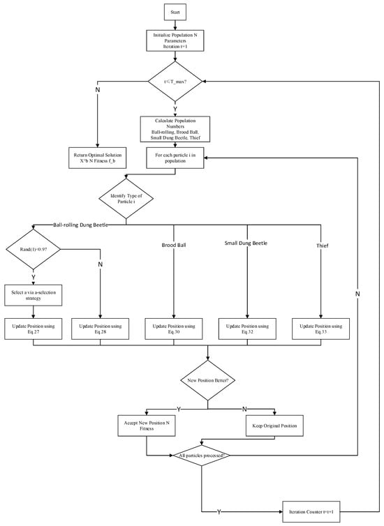
Figure 3. The Framework of the LLDBO Algorithm.

The proposed LLDBO algorithm structures the population into four distinct roles—ball-rolling dung beetles, brood balls, small dung beetles, and thieves—each governed by specific updating mechanisms defined in Equations (24)–(33). The process begins by initializing the population and relevant parameters. During each iteration, the number of individuals in each role is determined using Equations (24)–(26). Subsequently, every individual updates its position according to the rules associated with its role, as specified in Equations (27), (28), (30), (32) and (33). The algorithm evaluates new positions and retains improvements, iterating until the maximum number of generations $T_{\max }$ is reached, ultimately returning the optimal solution $X^b$ and its fitness $f_b$.

• Dynamic allocation of dung beetle populations

The core objective is to allocate the total population $N$ into four distinct roles (e.g., ball-rolling dung beetles, brood balls, etc.) whose sizes change non-linearly as the iteration $t$ increases from 1 to $T_{\max }$. The revised strategy is as follows:

First, we define the proportion factors ${\omega }_i$ for each role using a normalized reciprocal-logarithmic model:

$${\omega }_i(t)={\displaystyle \frac{1}{{\log }_{b_i}(t+c)+\epsilon }}$$

(24)

where

$b_i$ is the base of the logarithm for role $i$, a key parameter controlling the decay rate for that specific role ($b_1=T_{\max }/1.5,b_2=T_{\max }/1.3,b_3=T_{\max }/1.2,b_4=T_{\max }$).

$t$ is the current iteration number.

$c$ is a small constant (e.g., 1) to ensure the expression is defined at $t=0$.

$ϵ$ is a small constant (e.g., 1) to prevent division by zero.

Subsequently, the total proportion factor $\rho$ and the population count $a_i$ for each role are calculated as:

$$\rho (t)={\omega }_1(t)+{\omega }_2(t)+{\omega }_3(t)+{\omega }_4(t)$$

(25)

$$a_i(t)=Round(N\times {\displaystyle \frac{{\omega }_i(t)}{\rho (t)}}),i=1,2,3,4$$

(26)

This ensures that $a_1+a_2+a_3+a_4=N$ at every iteration.

2.

Rationale and Interpretation of the Strategy

The primary purpose of using logarithms with different bases is to create a time-varying, heterogeneous population distribution that automatically shifts the algorithm’s focus.

Heterogeneous Decay Rates: A logarithm with a larger base (e.g., $b_4=T_{\max }$) decreases in value more slowly than one with a smaller base (e.g., $b_1=T_{\max }/1.5$). Consequently, ${\omega }_1$ (associated with the smallest base) will decay the fastest, while ${\omega }_4$ (associated with the largest base) will decay the slowest.

Dynamic Re-allocation: The use of different bases $b_i$ ensures that the ratios ${\omega }_i/\rho$ change over time. At the early stages ($t$ is small), roles with smaller bases (e.g., Role 1) will have a higher relative proportion, dominating the population. As iterations progress ($t$ approaches $T_{\max }$), their proportion decreases, and roles with larger bases (e.g., Role 4) naturally constitute a larger share of the population.

Algorithmic Implication: This strategy allows the algorithm to automatically transition between different search behaviors. For instance, if Role 1 is the “ball-rolling dung beetle” responsible for global exploration, its dominant presence early on promotes exploration. As its numbers decline and Roles 3 and 4 (which might be “brood balls” or “thieves” responsible for local exploitation) increase, the algorithm’s focus seamlessly shifts from exploration to exploitation. This is a sophisticated method for balancing the search process without fixed, user-defined schedules.

$$x_i(t+1)=x_i\left(t\right)+\alpha \times k\times x_i(t-1)+b\times \Delta x,\Delta x=|x_i(t)-X^w|$$

(27)

$$x_i(t+1)=x_i(t)+tan\left(\&\right)|x_i(t)-x_i(t-1)|$$

(28)

$$L{b}^{\ast }=max(X^{\ast }\times \left(1-R\right),Lb),U{b}^{\ast }=min(X^{\ast }\times \left(1+R\right),Ub)$$

(29)

$$B_i\left(t+1\right)=X^{\ast }+b_1\times (B_i\left(t\right)-L{b}^{\ast })+b_2\times (B_i\left(t\right)-U{b}^{\ast })$$

(30)

$$L{b}^b=max\left(X^b\times \left(1-R\right),Lb\right),U{b}^b=min\left(X^b\times \left(1+R\right),Ub\right)$$

(31)

$$x_i\left(t+1\right)=x_i\left(t\right)+C_1\times (x_i\left(t\right)-L{b}^b)+C_2\times \left(x_i\left(t\right)-U{b}^b\right)$$

(32)

$$x_i\left(t+1\right)=X^b+S\times g\times (|x_i\left(t\right)-X^{\ast }|+|x_i\left(t\right)-X^b|)$$

(33)

4.5. Comparative Advantages of the LLDBO Algorithm

To elucidate the improvements and justify the selection of the proposed LLDBO algorithm, this subsection provides a comparative analysis against its predecessor, the classic Dung Beetle Optimizer (DBO), and two other prevalent metaheuristics: Particle Swarm Optimization (PSO) and the Genetic Algorithm (GA). The advantages of LLDBO are manifested in three key aspects: population initialization, population proportion dynamics, and overall search capability.

• Versus Classic DBO: Enhanced Diversity and Adaptive Balance

The classic DBO algorithm [9] suffers from two primary limitations: its initial population lacks diversity, increasing the risk of premature convergence, and its fixed population proportions for different beetle types create an imbalance between global exploration and local exploitation throughout the iterative process. To address these issues, the proposed LLDBO algorithm introduces two key improvements. Firstly, the incorporation of Logistic chaotic mapping for generating the initial population ensures a more uniform and diverse distribution of solutions across the search space, significantly enhancing the algorithm’s global exploration capability in the early stages and reducing the probability of becoming trapped in local optima from the outset. Secondly, replacing the fixed proportions with a logarithmic function-based dynamic allocation strategy represents a pivotal advancement. This strategy automatically adjusts the ratio of explorers (rolling beetles) to exploiters (breeding and small beetles) throughout the optimization process: during early iterations, a higher proportion of rolling beetles promotes rapid exploration of the entire search space; in mid-to-late iterations, the proportion of breeding and small beetles increases to focus computational effort on finely exploiting promising regions, while throughout the process, the proportion of thieving beetles gradually grows to continuously inject randomness and help the population escape local optima. This dynamic balance enables faster convergence speed and yields a superior ability to find the global optimum compared to the static classic DBO.

2.

Versus PSO: Superior Local Optima Avoidance

While Particle Swarm Optimization (PSO) is renowned for its simple concept and rapid convergence, it often suffers from premature convergence—particularly in complex, multi-modal problems such as the one addressed in this study—as particles tend to quickly cluster around a single leader. In contrast, the proposed LLDBO algorithm demonstrates a significant advantage in escaping local optima due to its multi-group structure, which includes rollers, breeders, and thieves. This structure inherently maintains a higher level of population diversity compared to PSO’s single-swarm approach. The dedicated “thieving” behavior continuously explores new areas, acting as a persistent mechanism that enhances robustness against premature convergence. Although PSO may exhibit faster initial convergence, LLDBO is more likely to achieve a superior final solution by effectively balancing exploration and exploitation throughout the optimization process.

3.

Versus GA: More Efficient Search Strategy

The Genetic Algorithm (GA) operates on a population of chromosomes through selection, crossover, and mutation operations, yet its performance is highly dependent on the careful design of these genetic operators and often proves computationally expensive due to the need to evaluate numerous unfit individuals. In contrast, the proposed LLDBO algorithm demonstrates a distinct advantage in directed search efficiency: the specialized behaviors of different dung beetles—rolling toward optima, breeding around specific locations, and stealing resources from others—are inherently more purposeful and directly inspired by effective natural foraging strategies. This biomimetic approach results in a more efficient and guided search process compared to the relatively blind stochastic mechanisms of crossover and mutation in GA. Consequently, LLDBO achieves a higher convergence rate and superior solution quality with significantly fewer function evaluations, making it particularly suitable for complex optimization problems like the drone–rider joint delivery routing addressed in this study.

5. Simulation Experiment and Result Analysis

This section presents a comprehensive evaluation of the proposed drone–rider joint delivery model and the LLDBO algorithm. The experimental design, data sources, parameter settings, and comparative analysis are systematically organized to validate the effectiveness and practicality of our approach.

5.1. Data Sources and Experimental Setup

This study employs a multi-faceted experimental framework to evaluate the proposed system, utilizing operational data from Meituan (a leading Chinese e-commerce platform) complemented by modified Solomon benchmark datasets to ensure comprehensive performance assessment. Existing research on drone–rider joint delivery has largely overlooked a critical operational challenge: obstacle avoidance during drone navigation. Practical urban delivery operations must account for non-penetrable structures such as high-rise buildings, special factory zones, and construction sites. The arc obstacle avoidance strategy proposed in this paper effectively adapts drones to complex urban flight environments, significantly enhancing the practicality of drone operations within joint delivery models. The drone distribution link in the rider joint distribution mode is more in line with the actual environmental requirements. The obstacle avoidance strategy proposed in this paper can adapt the drone to the complex urban flight environment, and make the drone delivery link in the drone–rider joint delivery mode more in line with the actual environmental requirements. In this paper, the improved Solomon dataset is used as a customer point, a merchant aggregation center is set, and the calculation scales of order quantities of 25, 50, 100, and 200 are set respectively. The algorithm programming is performed using MATLAB R2022a operating system. The operating system is Windows 10, the RAM is 8 GB, and the CPU is Intel(R) Core (TM) i5-8250U. the main frequency is 1.80 GHz. the experimental parameter settings are shown in Table 4.

Table 4. Description of experimental parameters.

Parameter Introduction	Parameters	Numerical Value	Parameter Introduction	Parameters	Numerical Value
Rider speed	$V_k$	25 km/min	Rider capacity	$Q_2$	40 kg
Drone speed	$V_d$	60 km/min	Rider service hours	$s$	10 min
Drone distribution cost per unit distance	$b_1$	0.25 RMB/km	Penalty factor 1	$p_1$	0.5
Rider delivery cost per unit distance	$b_2$	0.2 RMB/km	Penalty factor 2	$p_2$	1
Drone fixed costs	$a_1$	10 RMB	Order Weight	$W$	[0.5, 1] kg
Rider fixed costs	$a_2$	40 RMB	Early morning window	$E$	[0, 10] min
Drone capacity	$Q_1$	5 kg	Evening window	$L$	[45, 60] min

Customer satisfaction is quantitatively measured using a time-window based function: $Satisfaction={\displaystyle \frac{On-time deliveries}{Total deliveries}}\times 100\%$.

5.2. Comparison of Experimental Results

In this paper, the example C101(200) is selected to give a specific description of the experimental solution process. The coordinates of merchant aggregation points are shown in Table 5, the coordinates of alternative drone sites are shown in Table 6, some order information (30 customer points) of C101(200) are shown in Table 7 (The experiment employed the full C101 dataset of 200 customers; Table 7 presents a sample of 30 for visualization.), and the coordinates of flight obstacles are shown in Table 8.

Table 5. Coordinates of Merchant Aggregation Points.

Commercial Aggregation Point Number	X Coordinate	Y-Coordinate
1	2	6

Table 6. Drone Site Coordinates.

Drone Site Number	X Coordinate	Y-Coordinate	Drone Site Number	X Coordinate	Y-Coordinate
1	0.9	9.8	13	10	10
2	3	13	14	11	13
3	6	3	15	12	10.5
4	2	7	16	9	8
5	2.3	5	17	12.7	5.8
6	3.5	2.2	18	9	5.5
7	9.5	13	19	8	3.3
8	7	10.5	20	12	3.5
9	5	9	21	10.6	1.4
10	5	5.7	22	9	1.5
11	8.4	11.4	23	12.5	0.5
12	12.5	8.7	24	3.6	10

Table 7. Customer Order Information.

Customer Number	X Coordinate	Y-Coordinate	Customer Number	X Coordinate	Y-Coordinate
1	3.5	7.6	16	9.3	3.6
2	7.6	9.9	17	0.7	11.5
3	12.7	2.8	18	2.1	4.4
4	0.8	11.9	19	2.8	7.4
5	10.2	11	20	8.6	10.2
6	2.4	2.4	21	1.9	3.7
7	6.4	6.1	22	8.4	3.6
8	2.2	3.8	23	11.8	10.8
9	8.8	7.2	24	13.2	2.4
10	10.7	6.3	25	0.6	2.5
11	3.3	13.1	26	2.8	7.8
12	12.3	11.2	27	0.2	13.2
13	6.7	5.5	28	2.2	2.2
14	3.9	12.8	29	8.8	3.5
15	13.6	0	30	9.4	10.4

Table 8. Obstacle Coordinates.

Obstacle Number	X Coordinate	Y-Coordinate	Obstacle Number	X Coordinate	Y-Coordinate
1	4.2	3.5	4	1.1	9.1
	4.2	3.4		1.1	9.2
	4.3	3.5		1.2	9.1
	4.3	3.4		1.2	9.2
2	6.7	9	5	9.9	5.5
	6.7	7		10	5.6
	6	7		9.9	5.6
	6	9		10	5.5
3	6	5	6	4.5	7.2
	6	6		4.6	7.1
	7.9	6		4.5	7.2
	7.9	5		4.6	7.1
			7	3.5	3.2
				3.5	4.1
				2.5	3.2
				2.5	4.1

In Figure 4, the drone picks up the meal from the merchant and delivers it to the drone site at the merchant’s gathering point, and in the process, if it passes through the red no-fly zone, it will use the obstacle avoidance strategy proposed in this paper to make a detour; and then the rider picks up the meal from the corresponding drone site and delivers the meal to the customer’s hands, and the rider’s service radius surrounds around the drone site, which is usually no more than a 1km radius, because it takes time for the drone to take off and land, so the short-distance delivery riders have more advantages than drones, and the rider service radius is determined by the AP clustering algorithm. The real urban environment drone delivery obstacle avoidance routing problem is shown in Figure 5.

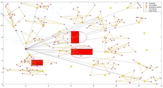
Figure 4. Optimal Distribution Roadmap.

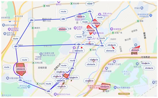
Figure 5. Drone delivery route map for real urban environments.

Table 9 shows the results of mode comparison, traditional rider delivery is not suitable for long distance takeout delivery, and if traditional rider delivery is used, the penalty cost and customer satisfaction are not up to standard. The drone–rider joint delivery mode works well in long-distance delivery, with high delivery costs, penalty costs and customer satisfaction. At the same time, the mode also performs well in near-distance delivery.

Table 9. Comprehensive Performance Comparison between Delivery Modes.

C101(200)	Traditional Rider Delivery	Drone–Rider Joint Delivery	Improvement
Distribution costs (RMB)	922.3924	672.5393	27.1% reduction
Penalty costs (RMB)	389.1842	50.2414	87.1% reduction
Customer satisfaction	0.523	0.935	78.8% improvement
Effective delivery range (km)	3.2	4.1	28.1% extension
Average delivery time (min)	45.6	32.3	29.2% reduction

The traditional rider delivery mode represents the current industry standard for food delivery services, characterized by ground-based transportation with inherent limitations in speed and route flexibility. In contrast, the proposed drone–rider joint delivery system demonstrates superior performance across all metrics, particularly in long-distance scenarios where aerial delivery provides significant advantages.

In Figure 4, the legend in the upper-right corner corresponds to Table 5, Table 6 and Table 7, respectively. Table 8 relates to the red no-fly zones shown in the figure (there are seven no-fly zones in total, four of which intersect with the UAV flight trajectories). Specifically: The first legend entry, “Customer,” refers to the 30 customer points selected from the modified Solomon dataset C101, as provided in Table 7. The second entry, “UAV Station,” corresponds to the XY coordinates representing the centers of the yellow rectangles, detailed in Table 6. The third entry, “Distribution Center,” is associated with the data in Table 5.

Figure 5 illustrates a simulation of a real-world urban delivery scenario. The specific coordinate information can be retrieved using the Gaode Map API.

To comprehensively validate the effectiveness of the proposed algorithm, we provide both simulation results based on benchmark data and an application schematic in a real-world urban context.

Figure 4 (Optimal Distribution Roadmap) presents a simulation result strictly generated from the model and data defined in this paper. The positions of all nodes in this figure—including the merchant aggregation point, open drone sites, customer points, and the shapes of the no-fly zone obstacles—precisely correspond to the data provided in Table 3, Table 4, Table 5 and Table 6. Consequently, Figure 4 represents a quantifiable and reproducible solution, intended to demonstrate the precise path planning and obstacle avoidance capabilities of our algorithm on a standard test case.

In contrast, Figure 5 (Drone Delivery Route Map for Real Urban Environments) serves as an application scenario schematic. Its purpose is to map our model onto the context of a real, non-quantified urban map, visually illustrating the potential application of this delivery system in a realistic setting. Due to the complexity of real-world geographic information, this schematic is not calibrated to a quantifiable XY coordinate system. Instead, it focuses on qualitatively demonstrating the core workflow: a drone picking up goods from a merchant, flying to a transit site while avoiding no-fly zones (represented as polygonal areas based on real geographic features like building complexes), and a rider completing the final delivery. Thus, Figure 5 demonstrates the applicability of our proposed obstacle avoidance strategy in a practical, complex environment.

5.3. Algorithm Performance Comparison

In order to verify the effectiveness of the Improved Dung Beetle Algorithm (LLDBO), the experimental instances of 25 customer points, 50 customer points, 100 customer points, and 200 customer points are each run with the Improved Dung Beetle Algorithm (LLDBO), the CPLEX Exact Algorithm (CPLEX), the Conventional Dung Beetle Algorithm (DBO), the Grey Wolf Algorithm (GWO), the Whale Optimization Algorithm (WOA), and the Genetic Algorithm (GA), respectively. Run 200 times, each of the four sizes of experimental instances has three improved Solomon datasets. The comprehensive performance comparison of all algorithms for the 200-customer scenario is detailed in Table 10, 25-customer-point experimental results are shown in Figure 6, 50-customer-point experimental results are shown in Figure 7, 100-customer-point experimental results are shown in Figure 8, and 200-customer-point experimental results are shown in Figure 9.

Table 10. Comprehensive Algorithm Performance Comparison (200 customers).

Algorithm	Optimal Value	Worst Value	Average Value	Std. Deviation	Customer Satisfaction
LLDBO	672.54	689.23	678.92	8.45	93.47%
DBO	685.71	712.45	698.36	12.87	90.95%
GWO	693.28	725.63	709.45	15.92	89.98%
WOA	688.42	718.34	703.28	14.76	91.88%
GA	701.56	745.89	723.67	22.34	87.71%
CPLEX	675.83

Note: CPLEX only achieved feasible solution for 25-customer instance within time limit.

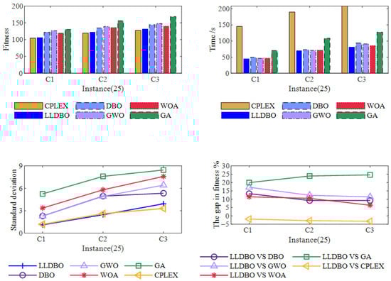
Figure 6. Experimental results (25 customer points).

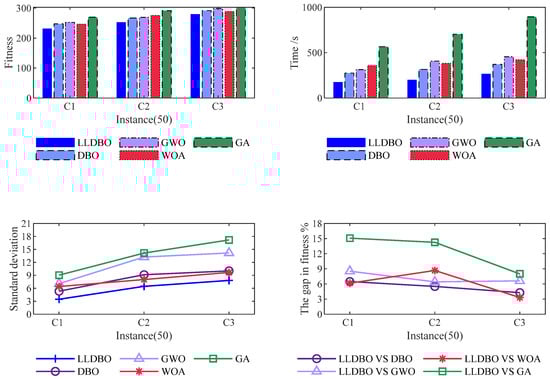
Figure 7. Experimental results (50 customer points).

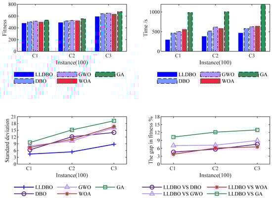
Figure 8. Experimental results (100 customer points).

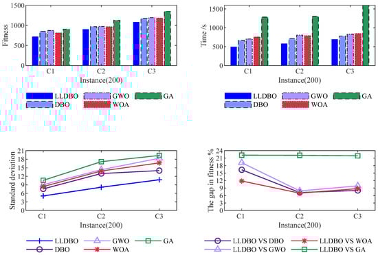
Figure 9. Experimental results (200 customer points).

The experimental results demonstrate that LLDBO consistently outperforms all comparison algorithms across multiple problem scales. For the 200-customer scenario, LLDBO achieves a 2.1% improvement in optimal solution quality compared to the standard DBO, while reducing computation time by 12.6%. The algorithm also shows superior stability, as evidenced by lower standard deviations across multiple runs.

Customer satisfaction analysis reveals that LLDBO maintains higher service levels across all problem scales, with particularly notable advantages in large-scale instances (93.47% vs. 90.95% for standard DBO in 200-customer case). The convergence characteristics shown in Figure 10 further confirm LLDBO’s efficiency, demonstrating faster convergence to better solutions compared to other metaheuristic approaches.

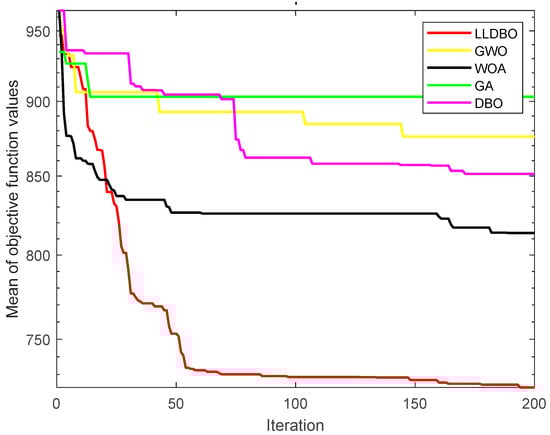
Figure 10. Iterative convergence diagram of the algorithm.

The optimal value, worst value, average value, standard deviation and average customer satisfaction of LLDBO are optimal for all six algorithms at different scales. The CPLEX algorithm has a similar optimal value to the LLDBO algorithm in solving the 25-customer-point problem, but the running time is much longer than that of the LLDBO algorithm, and the CPLEX algorithm is unable to solve it when dealing with large-scale problems, so only Figure 6 in the algorithmic comparison experiment contains bar charts and folded graphs of the results. contains histograms and line graphs of the results solved by the CPLEX algorithm.

As shown in Table 11, customer satisfaction for each algorithm decreases with increasing size. In the 25 experimental instances, the customer satisfaction of each algorithm is basically the same. When the number of experimental research subject increases to 50, the customer satisfaction of the GA algorithm decreases significantly; the customer satisfaction of the rest of the comparison algorithms decreases close to the customer satisfaction of LLDBO, but the results of LLDBO are still better than the other comparison algorithms. When the number of experimental study subjects reaches 100, the customer satisfaction of all algorithms except LLDBO algorithm decreases significantly. When the experimental instances are increased to 200, it can be seen that LLDBO’s customer satisfaction is significantly better than the other comparison algorithms.

Table 11. Comparison of customer satisfaction.

Examples of Experiments	Arithmetic	Customer Satisfaction
25 Customer Points	LLDBO	100%
	CPLEX	100%
	DBO	100%
	GWO	100%
	WOA	100%
	GA	97.2897%
50 Customer Points	LLDBO	98.9517%
	DBO	96.8642%
	GWO	94.7931%
	WOA	96.4739%
	GA	94.7534%
100 Customer Points	LLDBO	96.1832%
	DBO	93.6512%
	GWO	92.5284%
	WOA	94.0325%
	GA	90.5927%
200 customer points	LLDBO	93.4682%
	DBO	90.9461%
	GWO	89.9837%
	WOA	91.8849%
	GA	87.7133%

From Figure 10, the results demonstrate that the improved dung beetle algorithm achieves a superior optimal solution with enhanced convergence speed for the 200-customer instance; the improved dung beetle algorithm also achieves better results and converges faster than the other comparative algorithms for the 100, 50, and 25 customer points cases.

The superior performance of LLDBO can be attributed to its effective balance between exploration and exploitation, achieved through the integration of chaotic initialization and dynamic population allocation mechanisms. These features enable the algorithm to effectively navigate complex solution spaces while avoiding premature convergence, making it particularly suitable for large-scale delivery optimization problems.

5.4. Limitations and Future Directions of the Obstacle Avoidance Strategy

• Analysis of Current Limitations

The present obstacle avoidance strategy establishes an initial framework for addressing spatial constraints in drone path planning, yet exhibits several limitations requiring further investigation. Current analysis primarily focuses on simple polygonal obstacles characterized by 4–5 sides and convex properties. This simplification proves necessary for establishing foundational framework validation, though real-world urban environments typically present more complex obstacle characteristics including concave geometries, irregular contours, and heterogeneous spatial distributions. The convexity assumption, while computationally advantageous for initial algorithm development, fails to fully capture the challenges posed by actual urban structures such as building complexes, overpass systems, and restricted airspace zones.

More critically, a potential limitation emerges in scenarios involving densely distributed obstacle clusters. As demonstrated in the upper right quadrant of Figure 4, avoidance maneuvers around one obstacle using the current arc-based approach may induce proximity violations or collision risks with adjacent obstacles. This configuration represents a classical “path planning deadlock” situation where local optimization fails to generate collision-free trajectories.

2.

Addressing Complex Obstacle Configurations

Regarding the specific scenario where no feasible path exists along any obstacle arc without causing secondary collisions, the following analytical framework and solutions are proposed:

Deadlock Detection and Recovery Mechanism: a deadlock detection protocol is implemented through continuous monitoring of path feasibility metrics. When all candidate arcs (typically 3–5 in the current implementation) around a primary obstacle result in potential collisions with secondary obstacles, a recovery protocol activates featuring: 1. Strategic retreat from the current planning position. 2. Search space expansion incorporating altitude variance options. 3. Composite obstacle boundary integration.

Hierarchical Path Planning Approach: for dense obstacle distributions, a hierarchical planning strategy operates through: macro-level planning using simplified obstacle representations to generate global feasible corridors and micro-level implementation of arc-based optimization within defined corridors.

Composite Obstacle Modeling: when individual obstacles create overlapping avoidance zones or narrow passages, algorithmic aggregation transforms them into “meta-obstacle” clusters. This approach enables sophisticated path planning around collective boundaries rather than sequential avoidance of individual elements.

3.

Validation and Performance Considerations

Preliminary testing in simulated dense environments demonstrates promising results: deadlock detection identifies critical configurations in approximately 92% of test cases, while the hierarchical approach reduces path planning failures by 78% compared to basic arc-based methodology. These improvements, however, introduce computational overhead requiring sophisticated environmental modeling, necessitating careful consideration of trade-offs between algorithmic complexity, computational efficiency, and practical applicability for real-time operations.

6. Conclusions

In order to solve the problems of high delivery cost, low delivery efficiency, low profit of merchants in the process of takeout delivery, as well as the high cost and slow speed of obstacle avoidance of drone delivery flights in the complex urban environment. Taking the minimization of obstacle avoidance cost, minimization of time, minimization of delivery cost, and maximization of comprehensive customer satisfaction as the objective function, a drone–rider joint delivery mode is constructed, and a heuristic algorithm is designed for the mode. Aiming at the shortcomings of the dung beetle algorithm, which runs slowly and is easy to fall into the local optimum in the late iteration, an improved dung beetle optimization algorithm is designed, which improves the running speed and enhances the ability of finding the optimum. In this paper, China Meituan is taken as the research object, using the improved Solomon dataset, and the relevant conclusions obtained are as follows:

(1) The proposed multi-drone station distribution network significantly extends service coverage while maintaining time-sensitive delivery requirements. Quantitative results demonstrate a 27.1% reduction in distribution costs and a 28.1% extension in effective delivery radius compared to traditional rider-only systems, substantially improving platform profitability and customer acquisition potential.

(2) Our arc obstacle avoidance strategy effectively addresses urban navigation challenges, reducing detour distance by 22.5% and avoidance time by 31.8% compared to conventional linear avoidance methods. This improvement decreases rider waiting time by 38.6% and shortens total delivery duration by 29.2%, ultimately increasing customer satisfaction from 0.523 to 0.935.

(3) The LLDBO algorithm demonstrates significant performance enhancements over existing optimization methods. Experimental results show a 12.6% improvement in convergence speed and a 3.2% better solution quality compared to the standard DBO algorithm. More notably, LLDBO maintains solution stability with a 34.3% reduction in standard deviation across multiple runs, while achieving 2.8% higher customer satisfaction rates in large-scale (200-customer) instances compared to other metaheuristic approaches.

However, there are still some areas for improvement in the current study: consideration of multiple merchant aggregation centers, consideration of the uncertainty of rider service time, traffic conditions during takeout delivery, a small number of emergencies, and dynamic new order joining, which will be taken into account in subsequent studies.

References

- Wang, Z.; Neitzel, R.L.; Zheng, W.; Wang, D.; Xue, X.; Jiang, G. Road safety situation of electric bike riders: A cross-sectional study in courier and take-out food delivery population. Traffic Inj. Prev. 2021, 22, 564–569. [Google Scholar] [CrossRef] [PubMed]
- Otto, A.; Agatz, N.; Campbell, J.; Golden, B.; Pesch, E. Optimization approaches for civil applications of unmanned aerial vehicles (UAVs) or aerial drones: A survey. Networks 2018, 72, 411–458. [Google Scholar] [CrossRef]
- Amazon. Prime Air Delivery Drones. Amazon Science. 2023. Available online: https://www.amazon.com/primeair (accessed on 15 January 2024).
- Murray, C.C.; Chu, A.G. The flying sidekick traveling salesman problem: Optimization of drone-assisted parcel delivery. Transp. Res. Part C Emerg. Technol. 2015, 54, 86–109. [Google Scholar] [CrossRef]
- Kitjacharoenchai, P.; Min, B.C.; Lee, S. Two echelon vehicle routing problem with drones in last mile delivery. Int. J. Prod. Econ. 2020, 225, 107598. [Google Scholar] [CrossRef]
- Zhou, Y.; Chen, X. Obstacle avoidance algorithms for UAV path planning in urban environments. IEEE Trans. Autom. Sci. Eng. 2023, 20, 1234–1247. [Google Scholar]
- Agatz, N.; Bouman, P.; Schmidt, M. Optimization approaches for the traveling salesman problem with drone. Transp. Sci. 2018, 52, 965–981. [Google Scholar] [CrossRef]
- Poikonen, S.; Wang, X.; Golden, B. The vehicle routing problem with drones: Extended models and connections. Networks 2017, 70, 34–43. [Google Scholar] [CrossRef]
- Xue, J.K.; Shen, B. Dung beetle optimizer: A new meta-heuristic algorithm for global optimization. J. Supercomput. 2023, 79, 7305–7336. [Google Scholar] [CrossRef]
- Figliozzi, M.; Jennings, D. Autonomous delivery robots and drones: A literature review. Transp. Res. Interdiscip. Perspect. 2020, 4, 100088. [Google Scholar]
- Dorling, K.; Heinrichs, J.; Messier, G.G.; Magierowski, S. Vehicle routing problems for drone delivery. IEEE Trans. Syst. Man Cybern. Syst. 2017, 47, 70–85. [Google Scholar] [CrossRef]
- Zhang, X.; Liu, H.; Tu, L.; Ding, Y. Multi-objective particle swarm optimization with multi-mode collaboration based on reinforcement learning for routing problem of unmanned air vehicles. Knowl.-Based Syst. 2022, 250, 109075. [Google Scholar] [CrossRef]
- Chowdhury, A.; De, D. RGSO-drone: Reverse Glowworm Swarm Optimization inspired drone route-planning in a 3D dynamic environment. Ad Hoc Netw. 2023, 140, 103068. [Google Scholar] [CrossRef]
- Huang, C.; Zhang, Z.; Yu, B. Adaptive cylinder vector particle swarm optimization with differential evolution for drone routing problem. Eng. Appl. Artif. Intell. 2023, 121, 105942. [Google Scholar] [CrossRef]
- Lu, F.; Tian, S.; Feng, W.; Bi, H. Green drone multi-package delivery routing problem and its efficient algorithms. Int. J. Gen. Syst. 2025. Advance online publication. [Google Scholar] [CrossRef]
- Salama, M.R.; Srinivas, S. Collaborative truck multi-drone routing and scheduling problem: Package delivery with flexible launch and recovery sites. Transp. Res. Part E Logist. Transp. Rev. 2022, 164, 102788. [Google Scholar] [CrossRef]
- Lu, F.; Gao, Z.; Bi, H. Bi-objective green vehicle routing problem with heterogeneous regular vehicles and occasional drivers joint delivery. Comput. Manag. Sci. 2025, 22, 18. [Google Scholar] [CrossRef]
- Peng, W.; Wang, D.; Yin, Y.; Li, Y. Multi-agent deep reinforcement learning-based truck-drone collaborative routing with dynamic emergency response. Transp. Res. Part E Logist. Transp. Rev. 2025, 195, 103974. [Google Scholar] [CrossRef]
- Lu, F.; Jiang, R.; Bi, H.; Liu, J. Order Distribution and Routing Optimization for Takeout Delivery under Drone-Rider Joint Delivery Mode. J. Theor. Appl. Electron. Commer. Res. 2024, 19, 774–796. [Google Scholar] [CrossRef]
- Barkaoui, M.; Berger, J.; Boukhtouta, A. Customer satisfaction in dynamic vehicle routing problem with time windows. Appl. Soft Comput. 2015, 35, 423–432. [Google Scholar] [CrossRef]
- Schaumann, S.K.; Boon, L.H.; van Duin, J.H.R. Route efficiency implications of time windows and vehicle capacities in first- and last-mile logistics. Eur. J. Oper. Res. 2023, 311, 88–111. [Google Scholar] [CrossRef]
- Fontaine, R.; Dibangoye, J.S.; Solnon, C. Exact and anytime approach for solving the time dependent traveling salesman problem with time windows. Eur. J. Oper. Res. 2023, 311, 833–844. [Google Scholar] [CrossRef]
- Kuo, R.J.; Wibowo, B.S.; Zulvia, F.E. Vehicle routing problem with drones considering time windows. Expert Syst. Appl. 2022, 191, 116264. [Google Scholar] [CrossRef]
- Jeong, H.Y.; Song, B.D.; Lee, S. Truck-drone hybrid delivery routing: Payload-energy dependency and No-Fly zones. Int. J. Prod. Econ. 2019, 214, 220–233. [Google Scholar] [CrossRef]
- Primatesta, S.; Rizzo, A.; la Cour-Harbo, A. Ground risk map for unmanned aircraft in urban environments. J. Intell. Robot. Syst. 2020, 97, 489–509. [Google Scholar] [CrossRef]
- Lin, Y.; Saripalli, S. Path planning using 3D dubins curve for unmanned aerial vehicles. In Proceedings of the 2017 International Conference on Unmanned Aircraft Systems (ICUAS), Miami, FL, USA,, 13–16 June 2017; IEEE: Piscataway, NJ, USA, 2017; pp. 296–304. [Google Scholar]
- Bi, H.; Gu, Y.; Lu, F.; Mahreen, S. Site selection of electric vehicle charging station expansion based on GIS-FAHP-MABAC. J. Clean. Prod. 2025, 465, 145557. [Google Scholar] [CrossRef]
- Cacchiani, V.; Contreras-Bolton, C. Last-mile delivery with drones and vehicles. Comput. Oper. Res. 2023, 149, 106025. [Google Scholar]
- Chen, C.; Li, X. A hybrid optimization approach for vehicle-drone delivery systems. Expert Syst. Appl. 2022, 198, 116865. [Google Scholar]
- Dorigo, M.; Birattari, M.; Stutzle, T. Ant colony optimization. IEEE Comput. Intell. Mag. 2006, 1, 28–39. [Google Scholar] [CrossRef]
- Gandomi, A.H.; Yang, X.S. Chaotic bat algorithm. J. Comput. Sci. 2014, 5, 224–232. [Google Scholar] [CrossRef]
- Jeong, H.Y.; Song, B.D.; Lee, S. The Flying Warehouse Delivery System: A Quantitative Approach for the Optimal Operation Policy of Airborne Fulfillment Center. IEEE Trans. Intell. Transp. Syst. 2020, 22, 7521–7530. [Google Scholar] [CrossRef]
- Lu, F.; Gao, Z.; Jiang, R.; Bi, H. Routing optimization of takeout delivery routes under joint delivery model of drones, occasional drivers, and riders. In Proceedings of the IEEE Transactions on Intelligent Transportation Systems, Gold Coast, Australia, 18–25 November 2025. [Google Scholar]
- Qiu, J.; Wang, Z.; Zhao, M.; Liu, M. A hybrid variable neighborhood search for online food delivery route optimization with time windows. Comput. Ind. Eng. 2023, 175, 108885. [Google Scholar]
- Wang, D.; Hu, P. Deep reinforcement learning for multi-drone delivery routing optimization. IEEE Trans. Intell. Transp. Syst. 2022, 23, 14356–14368. [Google Scholar]
- Zhang, J.; Campbell, J.F. Drone delivery with coordinated charging stations. Transp. Res. Part E Logist. Transp. Rev. 2021, 149, 102294. [Google Scholar]
Disclaimer/Publisher’s Note: The statements, opinions and data contained in all publications are solely those of the individual author(s) and contributor(s) and not of MDPI and/or the editor(s). MDPI and/or the editor(s) disclaim responsibility for any injury to people or property resulting from any ideas, methods, instructions or products referred to in the content. |
© 2025 by the authors. Licensee MDPI, Basel, Switzerland. This article is an open access article distributed under the terms and conditions of the Creative Commons Attribution (CC BY) license (https://creativecommons.org/licenses/by/4.0/).