Deep Learning-Driven Parameter Identification for Rock Masses from Excavation-Induced Tunnel Deformations

Abstract

Efficient acquisition of rock mass parameters is a critical step for conducting numerical simulations in tunneling and ensuring the safety of subsequent construction. This paper proposes an intelligent back-analysis method for key rock mass parameters (Young’s modulus, Poisson’s ratio, cohesion, and friction angle) based on excavation-induced deformation data, using a deformation database that incorporates multi-feature values from tunnel excavation. This study employs five machine learning algorithms with single-feature inputs and three deep neural networks (DNNs) with multi-feature inputs, with a particular focus on convolutional neural network (CNN) due to their superior performance in terms of both accuracy and efficiency. The results demonstrate that the CNN model incorporating excavation features achieves excellent performance in parameter back-analysis, with an R² of 0.99 and 97.8% of predictions having errors within 5%. Compared with machine learning models using single-feature inputs, the CNN-based approach improves predictive performance by an average of 13.9%. Furthermore, compared with other DNNs, the CNN consistently outperforms across various evaluation metrics. This study also investigates the CNN’s capability to predict rock mass parameters using deformation data from early-stage excavation. After ten excavation steps, 96.9% of test samples had prediction errors within 5%. Finally, the proposed method was validated using field-monitored deformation data from a real highway tunnel project, confirming the method’s effectiveness and practical applicability.

1. Introduction

In tunnel engineering, the characteristics of the surrounding rock mass are among the most critical areas of study. This is particularly true under conditions of weak and fractured rock masses [1,2,3], where numerical simulations are essential for predicting potential issues such as excessive convergence, crown settlement, and stress concentration [4]. However, the complex behavior and inherent uncertainties of rock materials in constitutive modeling [5], make it challenging to obtain—accurately and efficiently—the mechanical parameters required for numerical simulations [6]. As rock mass physical parameters are among the key inputs in numerical models, insufficient accuracy may lead to significant safety risks during construction [7]. Therefore, timely evaluation of the rock conditions behind the tunnel lining and accurate acquisition of their mechanical properties are essential to ensure safe tunnel construction and subsequent support design [8,9].

Traditional methods for obtaining rock mass parameters primarily fall into two categories: (1) laboratory and in situ testing [6,10,11,12] and (2) numerical back-analysis methods [13,14,15,16,17]. While field or laboratory test results are often descriptive and may vary significantly depending on the sampling location, they are also constrained by site conditions and cost considerations. On the other hand, numerical approaches such as finite element or discrete element methods can provide an economical alternative for parameter estimation [18]. However, complex numerical modeling is often highly challenging and not feasible in large-scale engineering applications [19].

In recent years, the rapid development of artificial intelligence (AI) technologies has brought new opportunities to the field of geotechnical engineering [20,21,22,23,24,25]. Back-analysis methods based on monitoring data—such as displacement, stress, or strain—have also been widely used to estimate rock mass parameters [26,27,28,29]. At present, machine learning (ML)-based back-analysis methods have become one of the effective techniques for parameter estimation in geotechnical engineering [30]. Jia and Chi [31] used parallel mutation particle swarm optimization to perform back analysis of soil parameters for the Malutang II gravel dam. Chang et al. [32] proposed a MSVR algorithm based on the DE algorithm, where mixed data of stress and deformation were used for model training, showing better prediction performance than the single monitoring data DEMSVR model. Cui et al. [33] combined five machine learning algorithms to create a composite algorithm, selecting the model with the best performance for regression of different rock mass parameters. Zhang et al. [34] applied a BP neural network model optimized by the Mental Evolutionary Algorithm (MEA) for back analysis of rock mass mechanical parameters in a mining area.

However, in existing AI-based rock mass parameter back-analysis methods, the model inputs are generally based on a single feature point, which may result in the loss of critical deformation information related to the underlying parameter patterns during training. In any AI model, the selection of input features is crucial to the model’s performance [35]. Many civil engineering projects, such as foundation pits, slopes, and tunnels [36], involve multi-stage excavation. For instance, Sun [37] employed progressive excavation data as inputs to a back-propagation neural network (BPNN) surrogate model combined with Bayesian updating for slope displacement prediction. Zhang [38] introduced an Auto-Machine Learning model for predicting shield tunnel displacements induced by stepwise deep excavation. Dai [39] investigated model performance enhancement by incorporating excavation-related features in slope engineering and highlighted the feasibility of using excavation information as model inputs.

In this study, an efficient and intelligent back-analysis method for rock mass parameters is proposed based on deformation data induced by tunnel excavation. We validated the method using field-monitoring data from a highway-tunnel project. The key contributions of this study are as follows: (1) A novel approach is proposed for back-analyzing rock mass parameters using deformation feature values obtained after each excavation cycle. Unlike conventional back-analysis methods that rely solely on limited deformation data after excavation completion, the proposed approach fully utilizes the dynamic deformation information generated during the excavation process, thereby improving efficiency of parameter estimation. It is also more in line with engineering practice. (2) To the best of the authors’ knowledge, this study represents the first successful application of deep learning techniques to tunnel-related rock mass parameter back-analysis. This enables the back-analysis model to automatically learn the complex nonlinear relationship between deformation features and mechanical parameters, reducing the dependence on manual calibration features. (3) Another minor contribution, the tunnel deformation database constructed in this study explicitly considers excavation advance length and tunnel burial depth, which are often overlooked in prior works. The construction of the database provides a more comprehensive and real dataset for the training and verification of the model, and enhances the generalization ability of the method.

The structure of this paper is as follows: Section 2 describes the construction of the rock mass deformation database and outlines the different input strategies used for model development. Section 3 presents a comparative analysis of deep learning models using multi-point deformation features versus machine learning models based on single-point features, focusing on convergence deformation inputs. Section 4 evaluates the prediction accuracy of the convolutional neural network (CNN) model when using early-stage deformation data as input. Section 5 applies the proposed method to a real highway tunnel project and validates its performance using field-monitored deformation data. Finally, Section 6 concludes the study with key findings.

2. Methodology

2.1. Overall Workflow

The overall structure of the proposed method is depicted in Figure 1, providing a visual representation of the paper.

Step 1: The structural characteristics of a tunnel are typically determined by factors such as the excavation method, cross-sectional size, advance length, and burial depth. By combining these with multiple sets of rock mass parameters, a series of numerical models are established. Upon completion of the numerical simulations, deformation feature values—namely, crown settlement and convergence after each excavation cycle—are extracted at tunnel monitoring sections. These values are used to construct a tunnel deformation dataset comprising multiple characteristic points.

Step 2: Using the multi-feature-point deformation dataset generated from numerical simulations, the predictive performance of various models for rock mass parameters is evaluated. This study compares five commonly used machine learning models and three deep neural network architectures in terms of training accuracy and error performance. The results indicate that the Convolutional Neural Network (CNN) achieves the best predictive accuracy. Accordingly, CNN is further trained using early-stage (incomplete) deformation data of different types collected from individual tunnel sections, leading to the development of a CNN-based rock mass parameter back-analysis model.

Step 3: The trained model is applied to a real-world tunnel engineering project. Rock mass parameters are back-analyzed based on field-measured deformation data and subsequently used as input for finite element simulations. The simulated deformation results are then compared with actual field measurements to verify the prediction accuracy of the model.

2.2. Definition of FEM Tunnel Construction Conditions

This study is based on the proposed rock mass parameter back analysis method. For tunnel structures, if all conditions are divided by four influencing factors, the number of combinations becomes large. This makes it difficult to conduct the research effectively. Therefore, this paper constructs a tunnel deformation dataset under the assumption of fixed construction methods and cross-sectional size. Based on a real engineering case, a three-lane tunnel constructed using the upper–lower bench method is selected to validate the effectiveness of the proposed approach.

For the three-lane tunnel constructed using the upper-lower bench method, the classification is based on different levels of advance length and tunnel burial depth. The excavation speed is divided into four levels, and the burial depth is divided into eight levels, as shown in

Table 1. Classification of tunnel advance length and burial depth.

Tunnel Advance Length and Burial Depth
5 m	15 m	30 m		45 m	75 m		150 m	300 m		500 m
0.5 m/d			1 m/d			2 m/d			3 m/d

.

The most significant source of uncertainty in tunnel behavior arises from variations in rock mass quality. In this study, the classification of surrounding rock was conducted in accordance with the Technical Specifications for Highway Tunnel Construction. The specification defines physical parameter ranges for Classes III, IV, and V rock. To improve granularity and better reflect parameter sensitivity, these classes were further subdivided into subgrades. The classification method and corresponding physical parameter ranges are presented in

Table 2. Subdivision of rock mass classifications based on physical parameters.

Grade		γ (N/m3)	E (MPa)	μ	φ (°)	c (MPa)
III	III1	2550–2650	13,000–20,000	0.25–0.275	45–50	1.1–1.5
	III2	2450–2550	6000–13,000	0.275–0.3	39–45	0.7–1.1
IV	IV1	2375–2450	4500–6000	0.3–0.315	35–39	0.46–0.7
	IV2	2310–2375	3000–4500	0.315–0.33	31–35	0.33–0.46
	IV3	2250–2310	1300–3000	0.33–0.35	27–31	0.2–0.33
V	V1	1950–2250	1000–1300	0.35–0.4	20–27	0.125–0.2
	V2	1600–1950	500–1000	0.4–0.45	10–20	0.05–0.125

.

We selected the upper, lower, and median values for each subclass of surrounding rock as back-analysis targets for the rock mass parameters. We additionally introduced a set of randomly mixed parameters. This resulted in a total of sixteen distinct parameter sets. This strategy was adopted to enhance the representativeness and generalizability of the surrounding rock deformation database. By further combining these parameter sets with key influencing factors, tunnel burial depth and excavation advance length, a comprehensive set of experimental schemes was formulated.

By integrating these diverse modeling conditions, a total of 512 tunnel construction scenarios were generated. For each scenario, a three-dimensional numerical model was developed with FLAC3D. The full excavation process was simulated, and the complete deformation curves of the surrounding rock were extracted. The detailed modeling procedure is presented in Section 2.3.

2.3. Finite Element Modeling

Figure 2 shows finite element model and mesh configuration. The model domain measures 120 m × 90 m × 30 m and is discretized with hexahedral elements. A refined mesh is applied in the core excavation zone. resulting in a total of 175,560 elements and 183,976 nodes.

The Mohr–Coulomb failure model was adopted to simulate the mechanical behavior of the rock mass. Although the Hoek–Brown criterion provides a more sophisticated nonlinear representation of rock-mass strength, the Mohr–Coulomb model was chosen because of its simplicity, well-defined parameters, and compatibility with conventional tunnel-design practices. The boundary conditions of the numerical model are illustrated in Figure 3a. Lateral boundaries were constrained in the horizontal direction, while the front and back surfaces were restricted along the tunnel excavation axis. The bottom surface was fixed, and gravity loading was applied to the entire model.

To simplify the model complexity under varying burial depths, an upper-bound criterion was introduced to distinguish between shallow and deep burial conditions based on rock mass grade. The threshold depths for different rock grades were calculated using Equation (1) [40].

$$H_p=\left(2~2.5\right)\times \left(0.45\times 2^{S-1}\right)\times \left(1+i\left(B-5\right)\right)$$

(1)

$$F=\left(h-H_p\right)\gamma s$$

(2)

where Hp is the threshold depth used to distinguish shallow and deep burial conditions; S is the rock mass grade ranging from 1 to 5; B is the tunnel width (m); i is the pressure adjustment coefficient per meter of width, set to 0.12 for 14 ≤ B < 25; F denotes the equivalent surrounding rock pressure (N); h is the actual tunnel burial depth (m); and γ is the unit weight of the surrounding rock (N/m³); s is top area of model.

For shallow burial cases, the upper rock mass was removed and replaced with null, as shown in Figure 3c. In contrast, for deep burial scenarios, a load F, The calculation method is provided in Equation (2) [40]. F was applied on the top surface of the structure to simulate overburden stress, as shown in Figure 3b.

The support measures in the simulation model follow standard specifications and include a combination of shotcrete, rock bolts, and steel arches [14]. In this study, steel arches are modeled using struct liner elements in FLAC3D, with higher liner strength assigned to poorer rock mass grades.

The reinforcement effect of rock bolts is incorporated through equivalent parameter conversion into the shotcrete, by enhancing the physical properties of the rock mass within the bolt-anchored zone by a factor of 1.1. This value was adopted to conservatively represent this reinforcement effect. The invert backfill concrete is modeled using a linear elastic model, and its strength parameters are listed in

Table 3. Invert strength parameters.

γ (N/m3)	E (GPa)	μ
2400	28	0.2

.

2.4. Data Preparation

The full deformation curve of the tunnel crown is shown in Figure 4 [41]. This classical deformation profile can be divided into four stages: initial deformation, rapid deformation, slow deformation, and stress equilibrium. The most significant deformation occurs during the early portions of the rapid and slow deformation stages. Together, these two stages may account for more than 60% of the total surrounding-rock displacement. Therefore, deformation observed during these two stages is considered the most representative of the rock mass quality behind the tunnel lining.

In this study, characteristic deformation curves were extracted from each monitoring cross-section of the model after 3, 5, 10, and 15 tunnel excavation cycles to establish the analytical dataset [42]. The spatial layout of monitoring cross-section, as well as the distinction between monitored and predicted regions, is illustrated in Figure 4.

Figure 5 illustrates a sample from the tunnel deformation database used in this study. The seven crown settlement curves correspond to the median rock mass parameter values of the seven rock mass grades listed in Table 3. Other conditions are set as a burial depth of 15 m and an advance rate of 1 m per day. In Section 3, during the comparison of back-analysis models, the complete deformation curve was used as the input to the neural network. In Section 4, which focuses on CNN-based analysis with incomplete deformation data, different excavation stages correspond to different input points. For example, the 3rd excavation stage uses the green-marked points in the figure, whereas the 5th stage includes both the red and the green points.

3. Comparison of Back Analysis Models

3.1. Back Analysis Model Based on Excavation-Induced Tunnel Deformations

Deep learning is a subset of machine learning, and deep neural networks (DNNs) are a specific type of deep learning model [35]. A DNN consists of multiple hidden layers, where each layer performs a nonlinear transformation of data through neurons and weights. The workflow involves several key steps, including data input, forward propagation, error computation, backpropagation, and parameter updates [43].

In the forward propagation phase, each neuron receives input from the previous layer and performs a weighted summation using weights and biases. This process is mathematically expressed as follows:

$$y=f\left(\sum _{i=1}^n {\omega }_i{x}_i+b\right)$$

(3)

where $x_i$ represents the input features, ${\omega }_i$ is the weight, $b$ is the bias term, and $f$ is the nonlinear activation function. The weights ${\omega }_i$ and bias $b$ in the equation above are not derived from a direct calculation but are learned iteratively during the training process. This process begins with the random initialization of all parameters. Subsequently, the model undergoes forward propagation to make a prediction, and the error between the prediction and the true value is quantified by a loss function. The core of the learning lies in backpropagation, where the gradient of the loss function with respect to each weight, denoted as ${\displaystyle \frac{\partial L}{\partial \omega i}}$, is calculated. These gradients are then used to update the weights via a gradient descent optimization algorithm, following the update rule: $\theta {\displaystyle \frac{\partial L}{\partial \omega i}}\to {\omega }_i$, where $\theta$ is the learning rate. This cycle repeats until the model’s performance converges. The activation function introduces nonlinearity to the network, enabling it to learn complex data patterns. ReLU is commonly used as the activation function, and is defined as follows:

$$f_{ReLU}\left(x\right)=\left\{\begin{array}{c}x,x>0\\ 0,x\le 0\end{array}\right.$$

(4)

The three deep neural network architectures used in this study differ in structure [44].

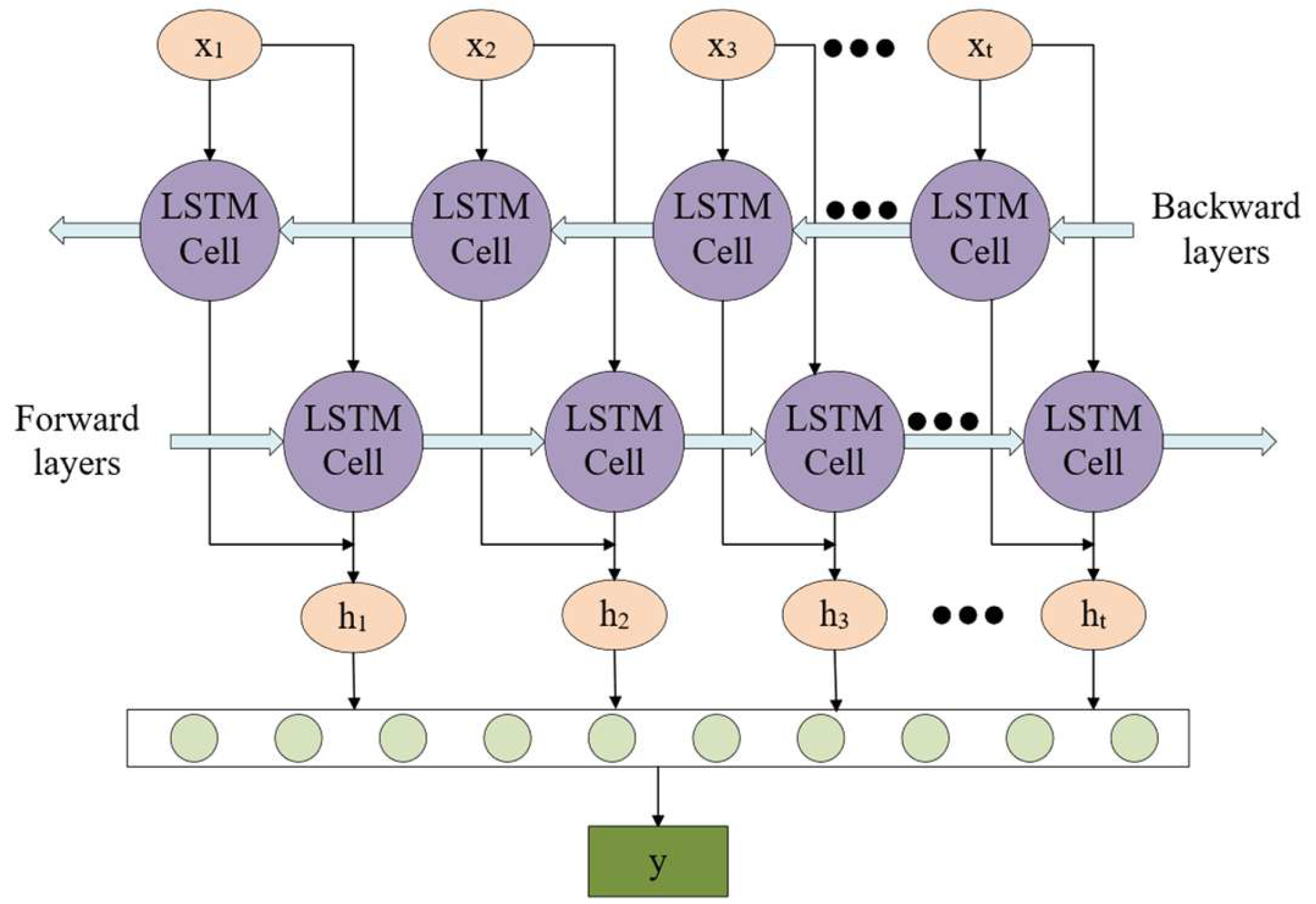
1. Bidirectional Long Short-Term Memory (BiLSTM): A BiLSTM consists of two independent LSTM units: one processes the sequence in a left-to-right direction, and the other processes the sequence in a right-to-left direction. An LSTM unit is composed of an input gate, forget gate, output gate, and cell state. The key equations for LSTM are as follows:

$$f_t=\sigma \left(W_f\cdot \left[h_{t-1},x_t\right]+b_f\right)$$

(5)

$$i_t=\sigma \left(W_i\cdot \left[h_{t-1},x_t\right]+b_i\right)$$

(6)

$${\tilde{C}}_t=\mathit{tanh}(W_C\cdot [h_{t-1},x_t]+b_C)$$

(7)

$$C_t=f_t\cdot C_{t-1}+i_t\cdot {\tilde{C}}_t$$

(8)

$$o_t=\sigma \left(W_o\left[h_{t-1},x_t\right]+b_o\right)$$

(9)

$$h_t=o_t\cdot \mathit{tanh}(C_t)$$

(10)

In the equations, $f_t$, $i_t$, $o_t$ and $h_t$ represent the forget gate, input gate, output gate, and hidden state, respectively. ${\tilde{C}}_t$ and $C_t$ represent the cell states before and after the update, respectively. $W$ and b are the weight vectors and bias terms, respectively. $h_{t-1}$ is the hidden state from the previous time step, and $x_t$ is the input at time step t. $\sigma$ is the sigmoid function, and tanh is the hyperbolic tangent function.

The input sequence is a one-dimensional time series $x\in R^{T\times 1}$. After processing by two stacked BiLSTM layers, the hidden state $H\in R^T\times 256$ is obtained, where the concatenated bidirectional output dimension is $2\times 128$. The final time step $h_T\in R^{T\times 256}$ is selected as the sequence representation and passed to a fully connected regression layer for prediction. The complete architecture of the network is shown in Figure 6.

2. Convolutional Neural Networks (CNNs) are a powerful deep learning model and the dominant architecture in the field of computer vision. They play an irreplaceable role in tasks such as image recognition, object detection, and image generation. CNNs use convolutional kernels to slide over the input data, calculating the weighted sum of local regions to generate feature maps, thereby performing local feature extraction on the input data. The mathematical expression for the convolution operation is as follows:

$$y\left(i,j\right)=\sum _{m=0}^{k-1} \sum _{n=0}^{k-1} x\left(i+m,j+n\right)\cdot \omega \left(m,n\right)+b$$

(11)

In the convolution operation, $x\left(i+m,j+n\right)$ represents a local region of the input data, $\omega \left(m,n\right)$ denotes the weight of the convolution kernel, $b$ is the bias term, and $k$ refers to the size of the convolution kernel. The configuration of the convolution kernel includes parameters such as kernel size, stride, padding method, and the number of kernels. The number of kernels determines the number of output feature map channels. By using local connections and weight sharing, CNN efficiently extracts features from the input data, providing rich feature information for subsequent layers of the network.

ResNet [45], a representative architecture of Convolutional Neural Networks (CNNs), addresses the gradient vanishing and information degradation issues in deep networks by introducing residual connections. The objective of the network learning is to predict the residual, F(x)=y−x, where y is the output and x is the input. Each Residual Block within the network is defined by the following basic computation:

$$y=F\left(x,\left\{Wi\right\}\right)+x$$

(12)

where x is the input (which can be the output from the previous layer), (x,{Wi}) is the nonlinear transformation within the residual block, and {Wi} represents the weights of the convolutional layers.

In this study, a deep neural network based on the ResNet50 architecture was primarily used to construct the rock mass evaluation model. The network is composed of an initial convolution and pooling layer, followed by a four-stage backbone, an average pooling layer, and a fully connected output layer. Each stage of the backbone includes multiple Residual Bottleneck Blocks along with a downsampling operation. The complete architecture of the network is shown in Figure 7.

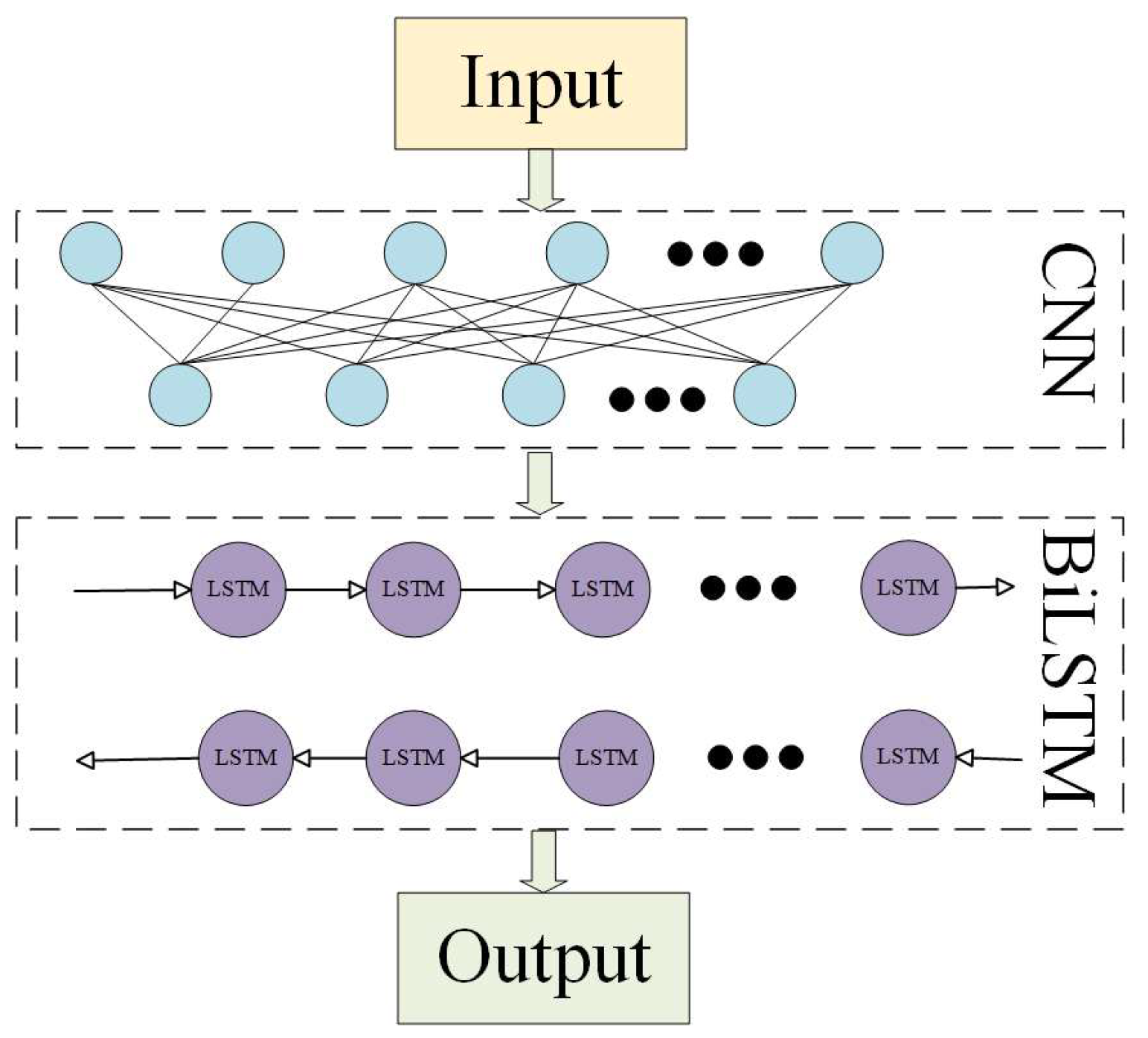
3. The CNN-BiLSTM model has been widely employed in image recognition and time-series analysis. It integrates Convolutional Neural Networks (CNNs) for spatial feature extraction and Bidirectional Long Short-Term Memory (BiLSTM) networks for temporal sequence modeling. Local spatial features are extracted by CNN, and temporal dependencies in both forward and backward directions are captured by BiLSTM. This combination enables the model to effectively represent spatial displacements and dynamic temporal variations. As a result, the architecture demonstrates reliable performance in complex sequence prediction tasks. The framework of CNN-BiLSTM is shown in Figure 8.

For all three models, Cross Entropy Loss is used as the loss function for classification tasks. The output logits are compared with the target labels to compute the loss [46].

The hyperparameters for the deep neural network models were selected based on grid search [47]. Specifically, hyperparameters were initialized with default values and then adjusted through experimentation [48]. The choice of hyperparameters has a significant impact on the model’s final performance. Models were trained with various hyperparameter settings, and the optimal hyperparameters for model were selected based on the best performance on the test set. Detailed information about the hyperparameters used in this study is provided in

Table 4. Deep Neural Network Hyperparameters.

Parameter	Set
Optimizer	ADAM
epochs	300
Size of the batch	32
Initial learn rate	0.0001
Learn rate drop period	100
Learn rate drop factor	0.1
Training set proportion	0.8

.

In the regression task, model performance is evaluated using three metrics: the coefficient of determination (R²), root mean squared error (RMSE), and the error rate within 5% [49]. The equations for evaluation are as follows:

$$R^2=1-{\displaystyle \frac{\sum \hspace{1em}(y_{\mathrm{true}}-y_{\mathrm{prediction}}{)}^2}{\sum \hspace{1em}(y_{\mathrm{true}}-y_{\mathrm{mean}}{)}^2}}$$

(13)

$$\delta$$

(14)

The training performance metrics of the three deep learning models are presented in

Table 5. Performance metrics for deep neural networks.

	R2			RMSE (GPa)
	Mixed	Convergence	Settlement	Mixed	Convergence	Settlement
CNN-BiLSTM	0.937	0.941	0.934	0.134	0.139	0.155
BiLSTM	0.913	0.913	0.922	0.231	0.223	0.333
CNN	0.996	0.994	0.994	0.032	0.033	0.039

, while the proportion of test samples with prediction errors within 5% is shown in

Table 6. Accuracy of different Deep Learning models.

	Accuracy (Error 5%)
	Mixed	Convergence	Settlement
CNN-BiLSTM	95.6%	94.9%	94.9%
BiLSTM	91.5%	90.9%	89.6%
CNN	97.8%	97.8%	95.6%

. The results indicate that the CNN model achieved the best performance during training, with all R² values exceeding 0.99 and the lowest RMSE reaching 0.033 GPa. It significantly outperformed both the CNN-BiLSTM and BiLSTM models. Across different input data types, the CNN-BiLSTM model consistently yielded lower RMSE values than the BiLSTM model. This demonstrates that the convolutional layers effectively enhance the model’s feature-extraction capability. In contrast, the standalone BiLSTM model showed relatively poor performance in this study, likely due to its reliance on strong temporal continuity in the input data. Furthermore, a comparison of training results using different input data types for the same model shows that mixed input data outperformed the cases where only peripheral convergence or vault settlement was used individually. Combined with the test set performance, these results indicate that using mixed data inputs provides the most significant improvement in model accuracy and generalization.

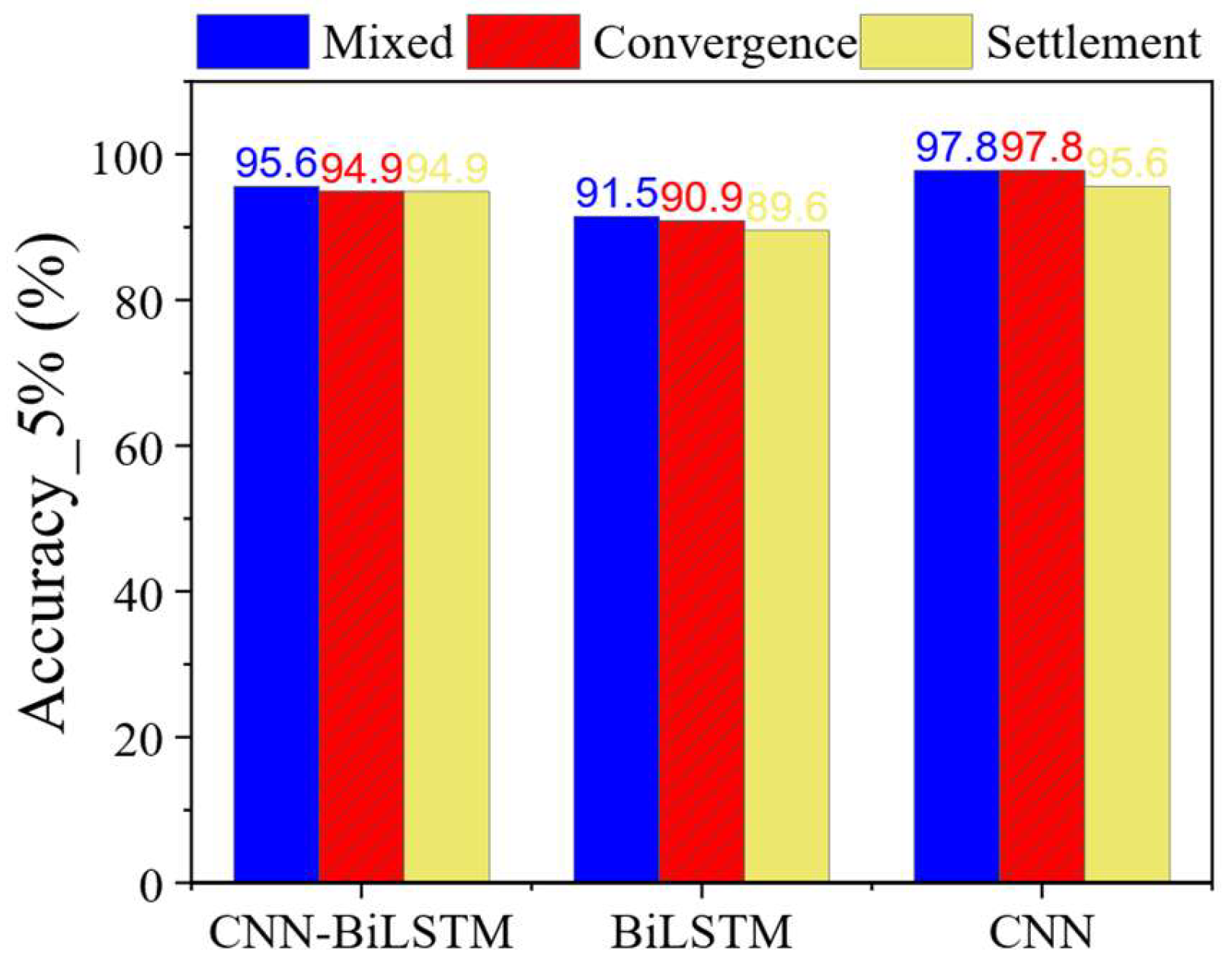
The CNN model also exhibited excellent performance on the test set. Across different input data types, the proportion of test samples with prediction errors within 5% reached up to 97.8%. Even when using only vault settlement as input, the proportion remained as high as 95.6%. In comparison, the BiLSTM model achieved a maximum accuracy of 91.5%. The CNN-BiLSTM model, which incorporates CNN-based feature extraction, achieved up to 95.6% under optimal conditions. These results indicate that the convolutional layers of CNN can effectively enhance BiLSTM’s learning capability by improving its ability to extract key features. This corresponds to an average increase of 4.3 percentage points.

As shown in Table 5, the CNN achieves R² = 0.996, 0.994, and 0.994. Such high values may signal a risk of overfitting in deep learning. We mitigated this by modifying the CNN training. We used AdamW with decoupled weight decay and applied an L2 penalty to convolutional and linear layers (weight decay = 1 × 10⁻⁵). Biases and normalization parameters were not regularized. We also used 10-fold cross-validation (k = 10) for train/validation splits.

Table 7. The k-fold cross validation index and confidence interval of CNN model.

	R2	95% CI	RMSE (GPa)	95% CI
Mixed	0.994724 ± 0.002577	[0.992881, 0.996567]	0.032247 ± 0.000387	[0.031971, 0.032524]
Convergence	0.984466 ± 0.010768	[0.973698, 0.995234]	0.033217 ± 0.000334	[0.032979, 0.033456]

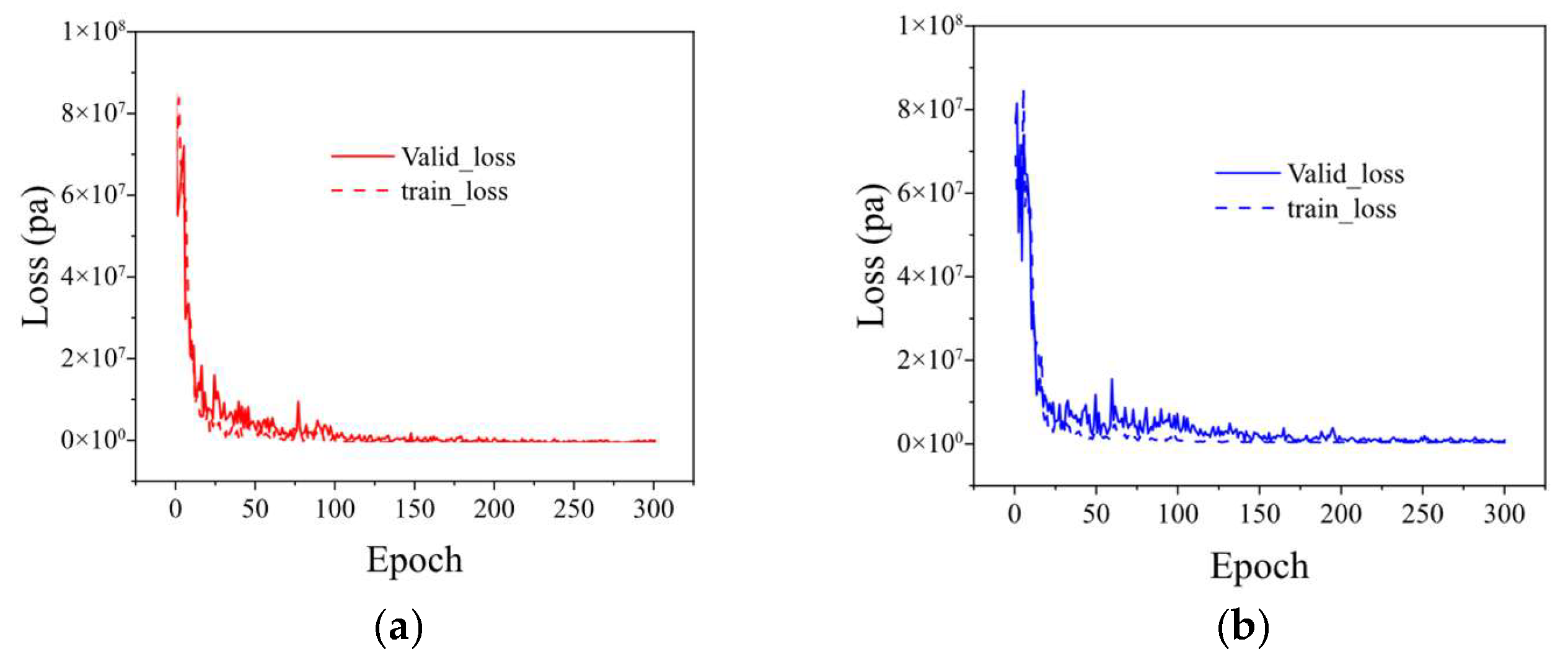
shows the CNN results with Mixed and Convergence inputs. R² = 0.994724 ± 0.002577 and 0.984466 ± 0.010768, respectively. The corresponding RMSE values are 0.032247 ± 0.000387 GPa and 0.033217 ± 0.000334 GPa. This paper also report 95% confidence intervals, computed with the t distribution (df = 9, t = 2.262). Compared with a single split, the 10-fold estimates provide a more reliable measure of generalization performance. The trends remain consistent with earlier findings: the CNN outperforms CNN-BiLSTM and BiLSTM. And mixed inputs yield additional gains. The learning curve (Figure 9) shows that the oscillation of the training loss becomes longer after the regularization is added, but from the final effect, the model performs well without the regularization technique and after the addition.

This paper attribute the superior performance of the ResNet50-based CNN to the nature of the input data, which consists of spatially distributed discrete measurement points with weak temporal correlations. Such data characteristics are better suited for CNNs, which excel at capturing local features rather than modeling temporal dependencies. Therefore, under this type of input, CNNs and their variants are able to achieve better predictive performance.

3.2. Back Analysis Model Based on Single-Feature-Point Deformation

Machine learning methods have demonstrated promising potential in the back analysis of rock mass parameters. To compare with the results of the deep learning model, five supervised algorithms previously used in back-analysis studies were selected, namely Decision Tree, Random Forest, Adaptive Boosting (AdaBoost), Support Vector Regression (SVR), and Backpropagation Neural Network (BPNN). Parameters for each algorithm were detailed in

Table 8. Algorithm settings for various Machine Learning models.

Model	Parameter	Value
DT	Criterion	entropy
	Max depth	8
	Min samples leaf	1
	Min samples split	2
RF	Max depth	8
	Min samples leaf	1
	Min samples split	2
	N estimators	100
AdaBoost	Estimator max depth	3
	Learning rate	1
	N estimators	100
SVR	C	10
	Gamma	0.1
	Kernel	rbf
	epsilon	0.1
BPNN	Batch size	32
	epochs	100
	Model dropout rate	0.1
	Model learning rate	0.001

.

The machine learning models adopted single-feature-point inputs, specifically the final convergence values of monitoring points. The training performance of different models is presented in

Table 9. Performance metrics for machine learning models.

	R2			RMSE (GPa)
	Mixed	Convergence	Settlement	Mixed	Convergence	Settlement
DT	0.839	0.831	0.833	0.697	0.611	0.699
RF	0.845	0.844	0.830	0.629	0.629	0.638
AdaBoost	0.852	0.850	0.842	0.359	0.388	0.459
SVR	0.811	0.811	0.801	0.308	0.338	0.408
BPNN	0.866	0.850	0.856	0.269	0.377	0.359

, while the proportion of test set errors within 5% is shown in

Table 10. Accuracy of different Machine Learning models.

	Accuracy (Error 5%)
	Mixed	Convergence	Settlement
DT	74.5%	71.8%	71.8%
RF	79.8%	71.8%	71.8%
AdaBoost	82.6%	71.8%	80.8%
SVR	84.5%	80.8%	75.4%
BPNN	84.5%	82.6%	80.8%

. The results demonstrate that among the machine learning models using single deformation feature points as input, the BPNN (Backpropagation Neural Network) exhibited the best performance. When trained with mixed-data inputs, it achieved the highest R² value of 0.866 and the lowest RMSE of 0.269 GPa. AdaBoost and SVR also delivered comparable results, with three models achieving over 80% of test set errors within a 5% margin.

The machine-learning models with single-feature-point inputs achieved a maximum test accuracy on the test set of 89.5%. The deep-learning models using multi-feature inputs reached 100% on the test set. When deep architectures were excluded, the best-performing model was SVR (Support Vector Regression). It achieved test-set accuracies of 84.5%, 80.8%, and 75.4% across different input data types, respectively. For models trained solely on crown settlement data, the maximum test accuracy was 81.8%, which was lower than those trained on the other two data types. In contrast, models using vault convergence data and mixed data exhibited comparable performance, suggesting that vault convergence data is of higher quality and demonstrates stronger correlation with the target variable.

3.3. Comparison of Different Parameter Back Analysis Methods

When trained with mixed input data incorporating multiple excavation-related feature points, the ResNet50-based model achieved an RMSE of 0.033 GPa. Compared with machine learning models using single-point inputs, the RMSE was significantly reduced, demonstrating the superior performance of the proposed approach. Furthermore, among all models utilizing multi-point inputs, the ResNet50-based CNN also yielded the lowest RMSE.

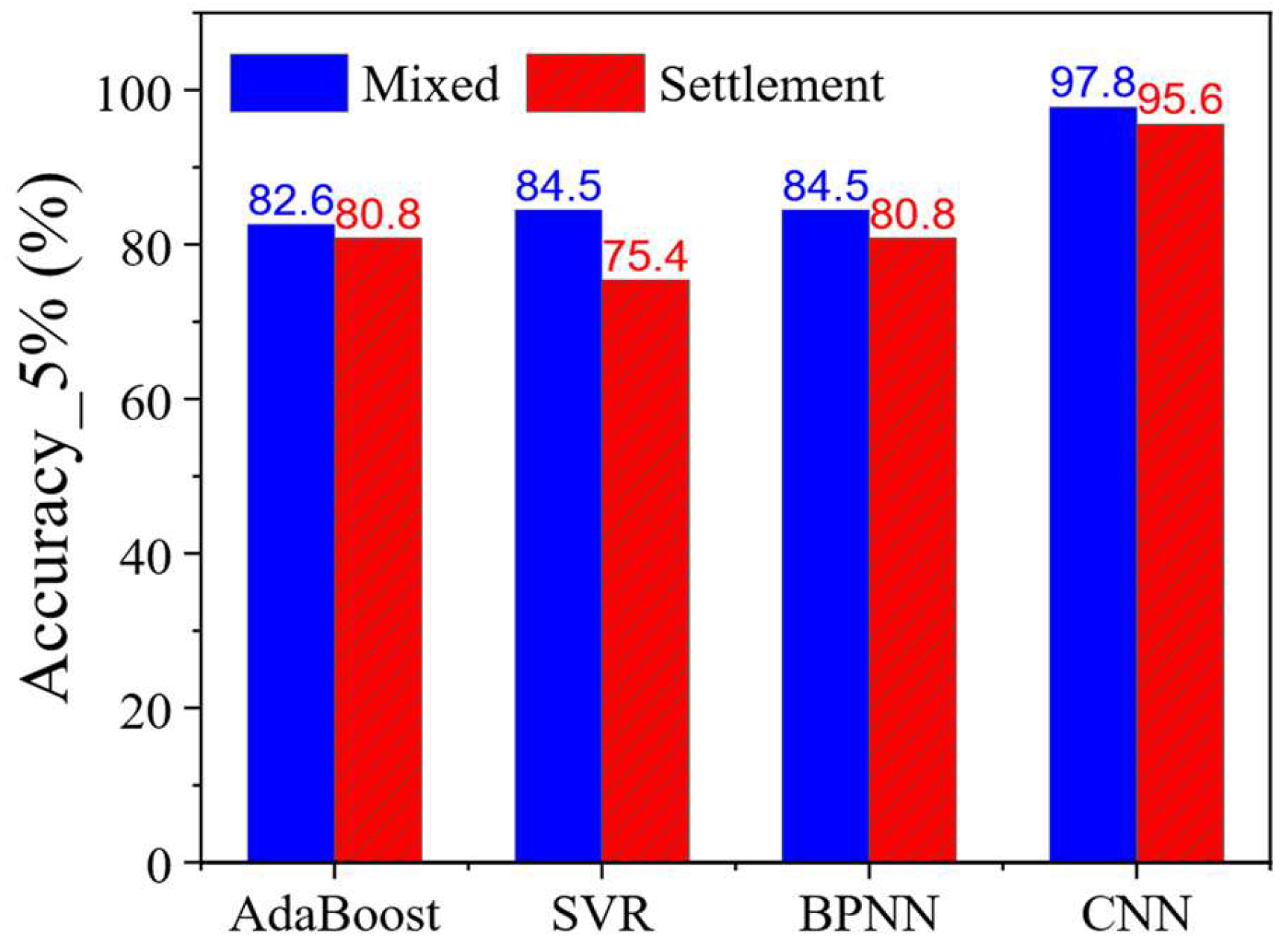
Figure 10 and Figure 11 illustrate the prediction accuracy (error within 5%) of the various models. It is evident that deep learning models incorporating multiple excavation feature points outperform others, with the ResNet50-based CNN slightly surpassing the other two deep learning models. In contrast, decision tree (DT) and random forest (RF) models showed poorer accuracy, likely due to the limited size of the training dataset or the shallow architecture, which constrains their ability to capture complex feature representations. Therefore, no comparison is made in Figure 11.

As shown in Figure 11, the models utilizing multi-point excavation features significantly outperform those using single-point inputs in terms of prediction accuracy. Compared with well-performing machine learning models such as BPNN and AdaBoost, the ResNet50-based CNN achieved an average improvement of 13.8% in accuracy.

In summary, the ResNet50-based CNN model demonstrates strong predictive capabilities and holds considerable potential for practical application in the back-analysis of rock mass mechanical parameters. The limitations of conventional machine learning models are mainly due to their shallow architectures, which cannot effectively capture the complex temporal and nonlinear patterns in deformation data. In contrast, DNNs offer a more robust solution [50]. DNNs can learn intricate, nonlinear relationships between excavation-induced deformation and rock mass quality, making them well-suited for back analysis tasks. Among the deep learning models, the CNN demonstrated the best performance when trained on complete deformation characteristic curves. Therefore, in Section 4, a modified ResNet50-based CNN was employed to analyze and discuss incomplete deformation curves, aiming to investigate the relationship between the CNN’s back-analysis accuracy and excavation progress under different input data types.

4. Efficient Back-Analysis of Physical Parameters Based on CNN

4.1. Model Training

This paper used the non-converged deformation values at different time intervals after rock excavation as inputs to the neural network model. Meanwhile, we investigated the influence of deformation at different positions around the tunnel crown on model performance. A total of 48 training runs were conducted using the CNN model. Training of the models required the use of GPU, and the hardware used in this study consisted of an NVIDIA A5000 GPU (NVIDIA, Santa Clara, CA, USA) and an Intel Xeon Gold 6346 processor (Intel, Santa Clara, CA, USA). With the sample dataset, the average training time for each model was approximately 25 min.

4.2. Training Results

Figure 12 shows the R2 scores of different models on the validation set. The results indicate that the average scores for the four regression parameters are 0.989, 0.991, 0.990, and 0.992, demonstrating that most models perform well not only on the training set but also converge well on the validation set.

Among the models, the lowest R² value occurred for the model trained on the third excavation feature dataset, regardless of whether crown settlement or convergence data were used. This model’s performance was consistently lower than that of the other models. Therefore, although the third excavation, which is closest to the monitoring point, theoretically has the greatest impact on the surrounding rock deformation at the monitoring point, the change in deformation after the first excavation does not provide sufficient distinguishing features for the CNN to achieve the rock mass back analysis effectively.

The RMSE values for different input data are shown in Figure 13. It can be observed that, for the same parameters, the smallest RMSE values are found in models trained with the mixed data. With the increase in the number of excavation feature points, the root mean square error (RMSE) of the back-analysis results shows an overall decreasing trend. The minimum RMSE values obtained for the four back-analysis parameters are as follows: Young’s modulus—3.16 × 10⁷ Pa, Poisson’s ratio—0.00146, internal friction angle—0.23048°, and cohesion—6105.11 Pa. when Young’s modulus is set as the back-analysis target and the deformation features after the tenth excavation step are used as input, the RMSE of the model using mixed data decreases by 20.5% compared to using convergence data, and by 231% compared to using settlement data alone. For the other back-analysis parameters—Poisson’s ratio, internal friction angle, and cohesion—the use of mixed input data leads to RMSE reductions of 14.2%, 21.8%, and 29.5%, respectively, compared with convergence data. Relative to vault settlement input, the reductions are even more significant, reaching 95.2%, 121.3%, and 301%, respectively.

These results indicate that Young’s modulus and cohesion are more sensitive to the type of input data, and that mixed data inputs significantly improve back-analysis accuracy.

Further analysis shows that, when mixed data are used as input, the RMSE of Young’s modulus prediction decreases consistently with the number of excavation feature points in Figure 13a. The corresponding RMSE values for the 1st, 5th, 10th, and 15th excavation steps are 6.96 × 10⁸ Pa, 2.69 × 10⁸ Pa, 8.07 × 10⁷ Pa, and 5.16 × 10⁷ Pa, respectively, with relative reductions of 111%, 236%, and 56%. The RMSE begins to stabilize between the 10th and 15th excavation steps. For comparison, when using the final convergence values of surrounding rock deformation as input, the RMSE is 4.3 × 10⁷ Pa. Beyond the 15th excavation step, additional feature points result in only a 20% further reduction in RMSE, indicating that the deformation information becomes saturated, and the marginal benefit of adding more features diminishes.

The R² score and RMSE reflect the overall performance of the model on the training set; however, they are not well suited for evaluating the dispersion of individual regression values. Using the ratio of prediction errors within 5% of the true values provides a more accurate measure of the model’s precision. As shown in Figure 14, It can be observed that regardless of the type of input data, the proportion of test samples with prediction errors within 5% increases as the number of excavation feature points grows. Taking mixed data as an example, when the deformation features from the ten excavation steps following the monitoring section are used as input, the prediction accuracies for the four back-analysis parameters reach 96.14%, 96.14%, 100%, and 95.63%, respectively. These accuracies are comparable to those achieved when the model is trained using convergence deformation values.

In contrast, when only vault settlement is used as input, the prediction accuracies after the tenth excavation step are 80.85%, 83.95%, 83.95%, and 80.85%, respectively—significantly lower than those obtained using mixed data. These results clearly demonstrate that incorporating mixed data as input substantially enhances the model’s performance.

5. Verification with Field Data

This study takes the portal section of a tunnel project in Zhejiang Province, China, as an engineering case for validation. The tunnel is 16.79 m wide and 10.85 m high. The selected section for geological monitoring is mainly in the V-grade rock mass zone. The ground above the tunnel consists of gravelly silty clay, underlain by weathered granite. The tunnel monitoring section is buried 20 m deep. Given the complex geological environment, the tunnel section under study was excavated and supported using the two-bench method.

Based on the highway tunnel rock mass classification scheme and combined with drilling and rock sample data, surface survey data, and engineering experience, a comprehensive classification of the rock mass was performed. The basic rock mass quality index modification value [BQ] for the tunnel monitoring section is calculated to range from 250 to 350. According to the [BQ] classification standards and relevant literature, the rock-mass grade was quantitatively determined to be Grade IV. Based on geological surveys, the qualitative classification was Grade V. During tunnel construction, the displacement of target points on tunnel cross-sections was monitored with a total station. The monitoring frequency was dynamically adjusted according to site conditions, as detailed in

Table 11. Tunnel monitoring frequency.

Monitoring Item	Monitoring Period	Monitoring Frequency
Rock Mass Deformation	N ≤ 10	2 times/day
	10 < N ≤28	1 time/day
	28 < N	1 time/week

Note: N refers to the number of monitoring days.

.

In the engineering validation stage, mixed data were used as input for the neural network. The back-analysis results trained with deformation features from ten excavation steps after the monitoring section are presented in

Table 12. Rock mass parameter prediction using 10th excavation data.

	E (MPa)	μ	C (MPa)	φ (°)	Grade
YK340	3080	0.338	0.560	30.48	IV2
YK380	2248	0.341	0.407	27.44	IV3
ZK340	3840	0.325	0.532	27.40	IV2

, while the results based on fifteen excavation steps are shown in

Table 13. Rock mass parameter prediction using 15th excavation data.

	E (MPa)	μ	C (MPa)	φ (°)	Grade
YK340	3170	0.339	0.568	31.66	IV2
YK380	2080	0.343	0.435	28.40	IV3
ZK340	3950	0.327	0.530	28.43	IV2

.

From the two tables, it can be observed that, among the rock mass parameters obtained through back-analysis using deformation features from different excavation steps, the Young’s modulus exhibits the most significant variation. For example, at section YK340, the back-analyzed Young’s modulus based on two different excavation stages is 3080 MPa and 3170 MPa, with a difference of 90 MPa. For the other two sections, the differences are 168 MPa and 110 MPa, respectively. In contrast, the variations in other back-analyzed parameters—such as Poisson’s ratio, internal friction angle, and cohesion—are relatively smaller, indicating that their sensitivity to excavation step differences is lower than that of Young’s modulus.

As a concrete check, Table 12 and Table 13 compare back-analysis results at the 10th and 15th excavation steps: the Young’s modulus varies by 90–168 MPa across sections (≈2.9–7.5%), while changes in Poisson’s ratio, internal friction angle, and cohesion are smaller, indicating that increasing stages beyond ten yields modest refinement rather than large shifts.

The numerical simulation results obtained from finite element models built using the back-analyzed parameters are shown in Figure 15. Figure 15 presents numerical results for crown settlement using back analysis parameters from different excavation feature points. At section YK340, the measured convergence deformation is 1.97 mm. The simulated convergence deformations based on the 10th and 15th excavation feature points are 1.98 mm and 1.82 mm, respectively, with a maximum error of 0.27 mm. At section YK380, which exhibits relatively poor rock mass conditions, the measured maximum deformation is 2.40 mm. The simulated values are 2.28 mm and 2.50 mm, with a maximum error of 0.12 mm. At section ZK340 in the left tunnel, the measured maximum deformation is 1.99 mm. The simulated values are 2.12 mm and 1.93 mm, yielding a maximum error of 0.13 mm. On average, the maximum error across the three sections is 0.17 mm, indicating good agreement between the simulation results and the actual crown settlement measurements.

6. Conclusions

This study proposes an intelligent back-analysis method for estimating rock mass parameters, in which the model input evolves from single-point to multi-point deformation features. Leveraging deep learning models, the approach enables faster and more accurate prediction of rock mass mechanical properties. The performance and practical applicability of the proposed method are validated using actual monitoring data from a highway tunnel project. This method provides a new idea for how multi-stage deformation characteristics reflect the mechanical behavior of surrounding rock, and provides a data-driven solution for more reliable tunnel safety analysis and evaluation. The main conclusions are as follows: (1). The deep learning-based back-analysis model with multi-point deformation inputs demonstrates higher prediction accuracy, achieving an average performance improvement of 13.8% compared to traditional machine learning models trained with single-point inputs. (2). The method allows for accurate estimation of rock mass parameters based on early-stage monitoring data. Reliable results can be obtained after ten excavation steps at a monitored tunnel section. (3). The type of input data significantly affects model performance. The use of mixed inputs—crown–shoulder convergence and crown settlement—yields better results than using crown settlement alone. Compared with using only crown–shoulder convergence, the improvement is marginal. (4). Engineering validation shows that finite element simulations of crown settlement using back-analyzed parameters closely match the measured deformations. The average prediction error across three typical tunnel sections is only 0.17 mm, confirming the reliability and applicability of the proposed method in real-world tunneling projects.