On the Usability of Isolation Forest for 3D Mesh Analysis and Watermarking

Abstract

Three-dimensional assets have evolved into a pivotal element within the domains of electronic entertainment, medicine, and engineering. Unfortunately, 3D models comprise voluminous data, which is not readily amenable to analysis or to the application of simple algorithms. This study thoroughly analyses the usability of the classical Isolation Forest (IF) method as a novel instrument for 3D mesh analysis. Given the atypical nature of 3D model data, it was necessary to obtain the special multidimensional feature vector (FV) associated with each vertex. The FV codes information regarding the local curvature of the surface in the vicinity of the vertex. As demonstrated by experimental studies, the IF analysis is capable of detecting geometrical details, areas of dense, complex geometry, strong bends, and folds in the mesh. This finding indicates a significant steganographic potential, which prompted the authors to employ research findings in the domain of 3D mesh watermarking as a practical illustration. Thanks to IF, a new steganographic method was developed that is characterised by higher transparency, achieved by hiding data in areas of complex geometry. The study proves the high potential of IF for analysing and watermarking 3D models, representing a meaningful step toward broader applications of IF in this field.

1. Introduction

In the modern era, data play a pivotal role—it is increasingly common to hear that “data are the gold of the 21st century”. Datasets are analysed and processed from multiple perspectives, and a wide range of models and algorithms have been developed for their processing. One such method is Isolation Forest (IF), which is widely applied to anomaly detection in data. The original Isolation Forest was introduced at the IEEE International Conference on Data Mining in 2008 [1], and it was based on a recursive partitioning of space into two disjoint subsets.

An important step in the development of Isolation Forest was the work of Karczmarek et al. in 2020 [2], in which the classical recursive partitioning was enhanced with the k-Means algorithm. The contribution of Karczmarek’s team significantly advanced research on IF. In 2021, an article was published [3] where the k-Means algorithm was replaced with the Fuzzy C-Means method, and in 2022, a study appeared [4] that focused on constructing IF based on the Minimum Spanning Tree.

In 2023, the popular deep learning approach was combined with Isolation Forest in the work of Xu et al. [5]. Two years later, Gałka presented an optimisation of this method in [6]. IF has been successfully applied to a variety of tasks [7,8,9], and its simple operating principle—random partitioning of the space into subsets—makes the model competitive with other available solutions.

Three-dimensional models pose a significant challenge for the application of typical data-processing algorithms. Unlike in the case of a standard dataset consisting of separate observations with a fixed number of features that can be directly analysed, here the vertices (data points) are distributed in a highly irregular manner. This leads to difficulties in applying many algorithms, particularly those based on local neighbourhood analysis using a fixed-size window, as is commonly performed, for example, in sound analysis and the generation of the Mel spectrogram [10,11]. Performing the widely used Principal Component Analysis also proves problematic [12].

The problem with algorithms based on a fixed-size shifting window is as follows. In 3D models with irregular vertex distributions, it is challenging to determine an appropriate distance and direction for shifting the window. When working with images (e.g., in discrete convolution algorithms), the window can be shifted by 1, 2, or 3 pixels in the up, down, left, or right directions. In audio analysis, the step size can be set based on time, e.g., 1 s, 2 s, and so on. However, in the context of 3D meshes, there is no universally suitable shift distance that guarantees all vertices are covered. Two vertices can be positioned in arbitrary ways relative to each other, making fixed-window approaches unreliable.

In mesh analysis, we work with a single, static dataset—the number of vertices remains constant, with the exception of rendering methods based on tessellation and level of details. For this reason, methods such as Bayesian filters [13,14], which require a reference dataset for comparison, turn out to be unsuitable.

In the case of 3D models, the applicability of Isolation Forest appears limited due to the nature of the input data. The situation, however, changes fundamentally owing to the novel idea of combining feature vectors generated from the local mesh geometry with Isolation Forest. Representing the characteristics of the local geometry surrounding a given vertex in the form of a multidimensional feature vector enables the application of IF analysis.

The future vectors contain values of angles as coordinates. The angles were calculated between the normal vectors of the faces to which a given vertex belongs and the corresponding average normal vector. This approach encodes the local curvature near a vertex in the form of angle values. The dataset of future vectors can be analysed as a standard dataset from the machine learning domain. The key idea is to extract features from the vertices and work with them directly, rather than developing a sophisticated algorithm to fit the full 3D volumetric data.

The results demonstrate both the validity and usefulness of the algorithm, as the study revealed that IF is capable of detecting details such as fine geometric elements, regions with complex and dense meshes, or areas with pronounced curvature and surface folding. Disturbances affecting vertices in flat regions of a 3D model tend to cause noticeable degradation, whereas altering vertices on curved surfaces generally does not result in significant visual deterioration [15,16]. It is worth noting that such regions constitute only a small fraction of the entire mesh structure, in the same way anomalies represent only a small portion of the entire dataset.

The motivation for writing this article was to explore the usability of Isolation Forest for 3D mesh analysis. The feasibility of applying Isolation Forest in the context of 3D assets, and particularly 3D models, remains largely unexplored. The second objective of this study is to present the research findings in a practical context. The vertices identified by Isolation Forest demonstrate significant potential for steganographic applications. In particular, we examine their use in the domain of 3D mesh watermarking, a specialized branch of steganography. In addition, this paper provides detailed information on the preprocessing of vertices prior to the application of IF. The obtained results are both promising and noteworthy, and they may serve as a foundation for establishing a new direction in IF applications.

The main contributions of this research are as follows:

• The introduction of Isolation Forest as a novel instrument for analysing 3D mesh models;
• The extension of the steganography toolkit with Isolation Forest;
• The practical application of research results in the form of a new 3D watermarking method;
• Designing a new watermarking method that improves transparency by embedding additional data within dense geometric regions to achieve better payload concealment.

The remainder of this article is organized as follows: Section 2 reviews methods for 3D mesh analysis, outlines the most popular research directions concerning 3D models, and discusses modern watermarking approaches. Section 3 describes the 3D models used in the study, provides an overview of Isolation Forest, and demonstrates the practical feasibility of applying our research to watermarking, including all preparatory steps. The obtained results are presented and discussed in Section 4. The effectiveness of the proposed IF-based watermarking method is compared with other state-of-the-art approaches in Section 5. Finally, the conclusions drawn from the study are summarized in Section 6, and directions for future development are outlined in Section 7.

2. Related Works

Currently, one of the most popular research directions is the development of machine learning and artificial intelligence. Both fields fundamentally rely on the processing and analysis of datasets. However, the analysis of 3D models, understood as data analysis, remains relatively uncommon due to the specific nature of such data. The main ongoing research directions involving 3D models include, among others, the generation of 3D models from 2D images [17,18], the training of large language models to understand or interpret 3D structures [19], mechanical analysis of constructions [20], and 3D printing [21]. Three-dimensional steganography and watermarking are more niche research areas; nonetheless, the analysis of model structure plays a key role. Practically every study in this domain introduces new methods for analysing model vertices.

In [16], a 3D model watermarking method robust against geometric attacks was proposed. High robustness was achieved by transforming the model into a space invariant to scaling, rotation, and translation. For this purpose, the model’s vertices were divided into three subsets, one of which carried the watermark, and the other two subsets were used to build the invariant space. Parts of the watermark were embedded in regions with dense and complex geometry. The detection of these regions required an analysis of the local mesh curvature, which was performed by examining the normal vectors of the faces belonging to the neighbourhood of the processed vertex.

While [16] focused on robustness to geometric attacks, [22] explored statistical approaches. To reduce the visibility of the introduced modifications, mesh curvature analysis was also performed. Normal vectors were employed to compute feature vectors encoding information about the local surface curvature in the neighbourhood of each vertex. The watermark embedding process relied on modifying the distributions of vertex (positional vectors) norms, as the vertices were divided into k bins, where k corresponded to the bit-length of the watermark.

The research in [23] is another work in which the watermarking process of the 3D model is based on modifying the distribution of vertex position vector norms. The authors employed the concept of salient points as the basis for partitioning the model mesh. Specifically, Voronoi diagrams were used for segmentation, while a proprietary method based on the Auto Diffusion Function was applied for salient point detection. For each segment, k-bins histograms of vertex position vector norms were generated, into which a k-bit portion of the watermark was embedded, with one bit assigned to each bin. This approach is noteworthy for combining geometric segmentation with statistical embedding, although its reliance on salient point detection may affect robustness and generalizability.

In contrast, ref. [24] employed a multiresolution strategy. Using the 3D wavelet transform, the model was decomposed into a sequence of representations with decreasing resolution (i.e., levels of detail). In this study, the watermark bits were embedded into the transform coefficients corresponding to the lowest level of detail. Not all coefficients were modified, as the embedding also depended on the watermark bit value. Additionally, the method was enhanced with a strength parameter that defined the trade-off between imperceptibility and robustness. However, embedding into the lowest-frequency coefficients typically limits the embedding capacity.

More recently, ref. [25] proposed a fragile watermarking scheme, where the watermark was represented by a keyed-Hash Message Authentication Code (HMAC). The HMAC was generated based on the texture and the set of vertices forming the model. Before computing the HMAC, the least significant digit of each coordinate of the selected vertices was extracted and replaced with zero. The extracted digits were then subjected to a discrete wavelet transform (DWT), and the watermark was embedded into the resulting coefficients. Finally, the inverse wavelet transform (IDWT) was applied, the digits were restored to their original positions, and the model was reconstructed. This approach demonstrates high imperceptibility but requires high computational cost due to DWT and IDWT.

An interesting approach to watermarking was proposed in [26], where the computational paradigm of Genetic Algorithm (GA), and Karhunen–Loève Transform (KLT) were employed. Each vertex of the model was represented as an Embedding Unit (EU). This structure contains the vertex position coordinates (3 × 4 bytes = 12 bytes) and a 16-byte fingerprint generated based on all polygons to which the vertex belongs. Subsequently, 28 bytes of each EU, interpreted as 28 non-negative pixel values, were subjected to the KLT, resulting in 28 coefficients. Depending on the watermark length, m coefficients were selected for embedding. The embedding process itself consisted in solving a nonlinear equation using GA: $(c_1,c_2,c_3,\dots ,c_{28})=\mathrm{KLT}(g_1,g_2,g_3,\dots ,g_{28})$, where $c_i$ denotes the predefined KLT coefficients, $g_i$ represents a byte of the EU, and only $g_4,g_8$, and $g_{12}$ are modifiable, i.e., the least significant bytes (LSBs) of the x, y, and z coordinates of the vertex position.

3. Materials and Methods

3.1. Three-Dimensional Models

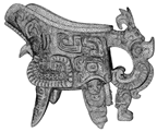
A wide variety of 3D models were employed in the research. As it is not feasible to list them all, the article focuses on eight models, which are presented in

Table 1. The part of the 3D models used in the research. The models are shown in the wireframe mode.

Model	Parameters	Model	Parameters
	Name: elephant		Name: ewer
	Size: 8761 KB		Size: 12,439 KB
	Vertices: 84,448		Vertices: 82,523
	Triangles: 149,768		Triangles: 149,999
	Source: 3D scan		Source: 3D scan
	Name: astronaut		Name: vase
	Size: 1779 KB		Size: 2939 KB
	Vertices: 51,096		Vertices: 52,446
	Triangles: 30,904		Triangles: 99,999
	Source: computer design		Source: 3D scan
	Name: cow		Name: pinecone
	Size: 18,151 KB		Size: 13,070 KB
	Vertices: 15,582		Vertices: 58,057
	Triangles: 29,345		Triangles: 100,000
	Source: computer design		Source: 3D scan
	Name: mannequin		Name: goat
	Size: 118 KB		Size: 131 KB
	Vertices: 1654		Vertices: 915
	Triangles: 2096		Triangles: 950
	Source: computer design		Source: computer design

. The selected objects represent different types of models, both in terms of mesh complexity and how they were created. As demonstrated in Table 1, the models under consideration comprise objects with hundreds of thousands of vertices (for example, the elephant and the ewer), as well as a low poly models with fewer than two thousand vertices (for example, the mannequin and the goat). This approach allows for a condensed presentation of the research results.

From the perspective of subsequent analysis, the file format and vertex attributes other than position are of negligible relevance. The present work concerns itself exclusively with the position attribute, which is expressed as a three-dimensional vector ($\overrightarrow{v}\in {\mathbb{R}}^3$). The files of all models used had the .glb extension, derived from the GL Transmission Format (glTF) standard, which is one of the most popular and accessible standards for storing 3D resources. It is acknowledged that certain models incorporated additional information, including textures or vertex attributes (e.g., normal vector and texture coordinates). However, these were excluded in alignment with the assumptions underlying the present study. The file sizes are provided for the sake of data completeness; however, it should be noted that these sizes are contingent on the presence of textures.

All models presented in Table 1 may be freely used for scientific, educational and non-commercial purposes. Models elephant (record ID: fsg_F1936.6a-b), ewer (record ID: fsg_F1961.33a-b), and vase (record ID: fsg_F1980.193a-b) come from The Smithsonian Institution (the “Smithsonian”, https://3d.si.edu/, accessed on 29 September 2025). Models mannequin (Animated Character Base by J-Toastie [CC-BY] via Poly Pizza, https://poly.pizza/m/AZzoJo1FBm, accessed on 29 September 2025) and goat (Cute Stylized Animal by MiniPoly [CC-BY] via Poly Pizza, https://poly.pizza/m/qBHcdCWqOM, accessed on 29 September 2025) come from the Poly Pizza website (https://poly.pizza/). The astronaut model (Z2 Spacesuit) comes from NASA’s online 3D models repository (https://science.nasa.gov/3d-resources/, accessed on 29 September 2025). The other models come from private sources.

3.2. Isolation Forest

Isolation Forest (IF), first presented at the IEEE International Conference on Data Mining in 2008 [1], aims to detect anomalies in datasets. The algorithm is based on the recursive division of space into two sets separated by a line in two-dimensional space, a plane in three-dimensional space, or a hyperplane in four and higher dimensions. The division process is recursive and continues until each set contains a single element or the assumed maximum division depth is reached.

The idea behind isolating observations is that anomalies in a set are a distinct minority and usually differ from normal observations. Anomalies often stand out from clusters of elements. Hence, the division process ends faster when there is an anomaly in a given branch. Normal values lie deeper/further in the structure.

According to the description provided, recursive partitioning generates a binary tree called an Isolation Tree (IT), and Isolation Forest is a collection of such trees. At each level of division, in a separate IT, one observation feature and any possible value of that feature are selected at random. The selected value constitutes the division boundary, whereby the feature must have a defined order so that it is possible to completely separate the observations into two subsets.

The training set for IF is the dataset itself, on the basis of which ITs are built, where the number of trees is the IF parameter. The prediction of observation $x_1$ (anomaly or normal value) consists of conducting a binary search of $x_1$ in each tree and calculating the anomaly score based on the average search depth.

3.3. Feature Vector

As is the case with many machine learning models, Isolation Forest requires a training set (i.e., a dataset) in order to function. In the case of 3D models, vertices are analysed, but a single vertex does not have features in the same sense as a single observation in standard training sets. Consequently, prior to the application of IF, it is necessary to prepare a dedicated feature vector (FV) for each vertex. Of course, it can be said that a vertex has attributes (e.g., normal vector and texture coordinates), and thus certain features. However, these elements primarily describe the visual aspects of the model. In particular, texture coordinates, in the context of geometry analysis, do not constitute a useful contribution.

In this work, the feature vector was generated in accordance with the approach described in articles [27,28,29], authored by other researchers. First, for each vertex, its nearest neighbourhood was determined, i.e., the set of vertices directly connected to it. This set is called valance. Next, only those vertices were selected whose neighbourhood has exactly p elements (valance of p-degree), where p is a parameter of the method and can be adjusted. In this work, $p=6$ was adopted (see Figure 1), because statistically, most vertices in 3D models have six neighbours [27,28,29]. Additionally, areas with simple, flat geometry are usually characterised by vertices with a valance of 8, which is associated with an accumulation of squares, each of which consists of two triangles. Nevertheless, the research also includes experiments involving $p=4, 5, 7$, and 8; the findings are presented in Section 4.

For each triangle (face) forming the valance of a vertex, a normal vector (a vector perpendicular to the surface, oriented outside the model) was calculated. Then, based on the normal vectors of the faces, the average normal vector was determined and assigned to the central vertex (see Figure 2). With the above data available, the feature vector $\overrightarrow{f}$ was determined for each vertex separately, according to Formula (1):

$$\overrightarrow{f_i}=arccos\left({\displaystyle \frac{{\overrightarrow{n}}_i·{\overrightarrow{n}}_{avg}}{\parallel {\overrightarrow{n}}_i\parallel \parallel {\overrightarrow{n}}_{avg}\parallel }}\right),\mathrm{for}i=0,1,...,p-1,$$

(1)

where ${\overrightarrow{f}}_i$ is the i-th coordinate of the feature vector (angle), ${\overrightarrow{n}}_i$ is the normal vector of the i-th face, and ${\overrightarrow{n}}_{avg}$ is the average normal vector. The numerator contains a dot product, and $\parallel ·\parallel$ is the length of the vector. Zero-based indexing was also used.

The coordinates of the feature vector correspond to the values of the angles between the normal vectors and the average normal vector, while the entire feature vector describes the local geometry in the vicinity of the vertex. Areas with flat, simple geometry are characterised by values of ${\overrightarrow{f}}_i\approx 0$, while areas with complex geometry are characterised by high values of ${\overrightarrow{f}}_i$. The set of FVs constitutes the input data for Isolation Forest.

Areas with flat, simple geometry are characterized by values of ${\overrightarrow{f}}_i\approx 0$, because in this case the face normals are nearly identical to the average normal vector, resulting in angles close to zero. Conversely, a local peak, ridge, or pronounced fold causes the face normals to diverge, producing a wide range of angle values. In this way, the feature vector encodes the local curvature of the geometry for IF analysis.

3.4. Vertex Analysis

The analysis of the model geometry involves the use of Isolation Forest for the feature vectors set. The study used the IF implementation from the scikit-learn package, available in Python 3.12.4. The model has three parameters—n_estimators (number of trees), contamination (percentage of outliers in the dataset), and random_state (seed)—which can be adjusted as needed. For each vertex, the anomaly score ($as\left(x\right)$) metric was calculated, and it was assumed that $as\left(x\right)<0$ indicates an anomaly.

Most of the vertices for which $as\left(x\right)<0$ are located in areas of complex and dense geometry (see Section 4 for more details). During the watermarking process, the additional data (watermark) is embedded in these regions.

The IF analysis should be deterministic for synchronized watermarking and verification; therefore, the random_state seed must be used and stored along with n_estimators and contamination. To preserve these values, the proposed watermarking method uses a steganography key that contains the aforementioned parameters.

Typical datasets used in machine learning often contain anomalies—abnormal values that may arise from momentary errors in measurement equipment or human mistakes. In contrast, anomalies in 3D models, such as those used in rendering, are seldom discussed. The concept of an anomaly is also difficult to define precisely, despite the frequent use of terms such as graphical artefact or glitch. Consequently, the output of IF does not represent a set of anomalies; rather, it is a set of vertices that share specific characteristics. It is important to emphasise that this resulting set depends on the previously constructed feature vector.

Isolation Forest operates on a feature vector whose components correspond to angle values expressed in radians. These values are in the range $[0,\pi )$, which is important because IF works best when features are on a similar scale (e.g., after min-max normalisation or standardisation).

3.5. Watermarking and Authenticity Verification

The vertices selected using the method described in Section 3.4 can also serve as potential locations for watermark embedding. The article [30] presents an efficient and non-intrusive method of marking 3D models, in which watermark bits are placed in randomly selected vertices.

The watermarking process in the cited work consists of four steps. In the initial phase, each component of the vertex position attribute ($\overrightarrow{v}\in {\mathbb{R}}^3$) undergoes a least significant bit (LSB) zeroing operation. This creates a new model, which is used to generate a Hash-based Message Authentication Code (HMAC) [31,32]. In the following step, vertices from the original model are selected at random, in which the watermark bits (HMAC code) are ultimately embedded.

The drawback of this approach lies in the lack of control over the choice of vertices where the data will be hidden. Random distribution of the watermark throughout the model results in a high probability of modifying flat regions or distinctive points, which is undesirable.

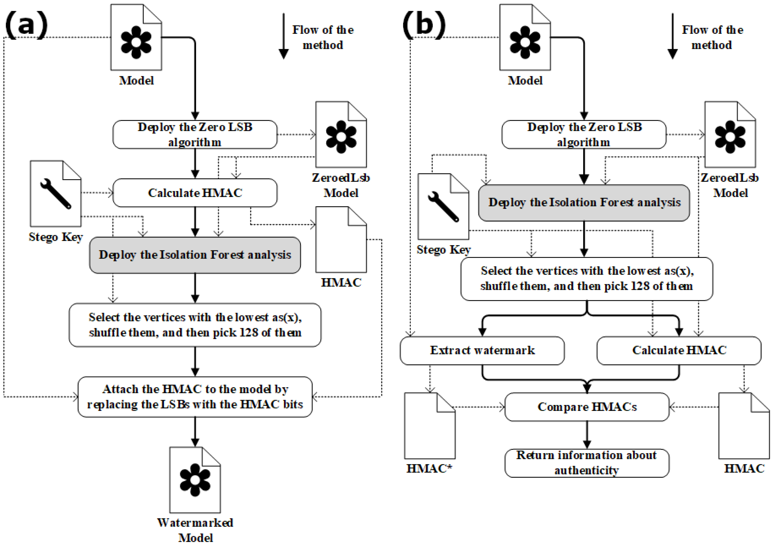
In the new proposed approach, vertices carrying the watermark are not selected randomly; rather, vertices selected using the IF analysis are used. As illustrated in Figure 3a, a novel methodology for embedding a watermark within a 3D model is presented, with the stage of the IF analysis highlighted.

The approach uses a steganographic key (Stego Key), i.e., a secret element containing information necessary for the correct marking of the model and subsequent verification of its authenticity. The Stego Key stores the following data: the values of the parameters random_state, n_estimators and contamination for Isolation Forest, the key for calculating HMAC, the HMAC length in bits, and the number picked for the shuffle stage.

The cryptographic hash function BLAKE2 [33,34] was used to generate the watermark, i.e., the HMAC code. The input data was the entire file containing the model with zeroed LSBs (marked as ZeroedLsbModel in Figure 3), and the length of the resulting HMAC was 48 bytes. Given that the watermark consists of 384 bits, it follows that only 128 vertices were modified (with each vertex possessing three coordinates, i.e., $384/3=128$).

From among the vertices selected by IF, those with the lowest anomaly score were selected, shuffled, and the first 128 were chosen. Prior to the execution of the shuffle, the generator seed was set to random_state. The number of instances with the lowest $as\left(x\right)$ values is an adjustable parameter, stored within the steganographic key. For example, one may initially select 400 vertices; however, if this is not feasible, attempts can be made to use 300, followed by 200, 150, 130, and finally 128 vertices. If the number of selected vertices falls below 128, the method cannot embed the entire watermark, and a shorter watermark must be generated. The length of the watermark is also stored in the Stego Key.

The watermark embedding process involves replacing the least significant bits (LSBs) of the positional coordinates of selected vertices with bits of the HMAC code. The position of a vertex is represented by a 3D vector $\overrightarrow{v}=(x,y,z)$, where each coordinate is a 4-byte floating-point number. During embedding, the LSB of each coordinate (x, y, and z) is modified by replacing it with a bit from the HMAC code.

Since an LSB can only be either 0 or 1, and we replace it with another 0 or 1, some LSBs remain unchanged (with a theoretical probability of 50% for a change). Thus, although we attempt to modify 384 values in total, in practice only a portion of these 384 bits are actually altered.

The verification process, i.e., watermark extraction, is illustrated in Figure 3b. First, for each positional coordinate of every vertex, the LSB is cleared, resulting in a temporary model (the original has not been modified). The proposed method is blind, meaning that the verification process does not require access to the original model. The key idea is to zero the LSBs before computing the HMAC code, both during embedding and verification. Because the LSBs are cleared before the HMAC is calculated, the authentication process produces the same HMAC value as in the watermarking phase.

Using the Stego Key, Isolation Forest analysis is then performed on the temporary model to identify vertices (indices), some of which contain HMAC code bits. This step is identical to the procedure used in the watermarking process. The next step is the shuffling stage, also carried out exactly as in the watermark embedding. The watermark is subsequently extracted from the vertices of the original model. A new HMAC code is generated based on the temporary model. Finally, the newly generated HMAC is compared with the extracted HMAC (in Figure 3 labeled as HMAC*). If the two bit sequences do not match, this indicates that the watermark has been removed, meaning the model has been modified.

3.6. Interference Measures

Standard vertex attributes, including position, normal vector, and texture coordinates, are vector values whose coordinates are real numbers. Consequently, most metrics, like Signal-to-Noise Ratio (SNR), Root Mean Square Error (RMSE), or Hausdorff Distance (HD), can be applied to each of these attributes. However, it should be noted that the normal vectors or texture coordinates are not pertinent to the objectives of the study. In this study, SNR, RMSE, and HD were utilized to assess the interference level introduced during the watermarking process of 3D models. The metrics that have been selected are the most frequently utilized ones [35].

SNR is a general measure of the ratio between the power of a signal and the power of background noise present in it. It is commonly expressed in decibels (dB). Mathematically, SNR is defined as [16]

$$\mathrm{SNR}=10·{log}_{10}{\displaystyle \frac{{\displaystyle \sum _{\overrightarrow{v}\in \mathbf{Y}}}{\parallel \overrightarrow{v}\parallel }^2}{{\displaystyle \sum _{\overrightarrow{v}\in \mathbf{Y}}}{\parallel \overrightarrow{v}-\overrightarrow{v^{\prime }}\parallel }^2}},$$

(2)

where $\overrightarrow{v^{\prime }}$ is a vertex of the modified model corresponding to $\overrightarrow{v}$, $\mathbf{Y}$ denotes the set of vertices of the original model, and $\parallel ·\parallel$ represents the Euclidean norm.

RMSE measures the average magnitude of the errors between the original and the watermarked model and is defined as the square root of the Mean Square Error (MSE) [36].

$$\begin{array}{cc}\hfill \mathrm{RMSE}& =\sqrt{\mathrm{MSE}},\hfill \\ \hfill \mathrm{MSE}& ={\displaystyle \frac{{\displaystyle \sum _{\overrightarrow{v}\in \mathbf{Y}}}\parallel \overrightarrow{v}-\overrightarrow{v^{\prime }}{\parallel }^2}{\left|\mathbf{Y}\right|}},\hfill \end{array}$$

(3)

where the symbol $\left|\mathbf{Y}\right|$ indicates the cardinality of the set $\mathbf{Y}$.

The Hausdorff Distance ($d_H$) quantifies the degree of dissimilarity between two subsets of a metric space. In computer graphics, it is commonly employed to assess the differences between two distinct representations of the same 3D object.

Let $S_1$ and $S_2$ denote the set of vertices (planes) of the modified and original models, respectively, then [37]

$$d_H=max\left(E(S_1,S_2),E(S_2,S_1)\right),$$

(4)

where $E(S_x,S_y)$ = $\underset{p\in S_x}{max}e(p,S_y)$ is the unilateral distance between two planes $S_x$, $S_y$, where $e(p,S)=\underset{p^{\prime }\in S}{min}d(p,p^{\prime })$ is the distance between point p and plane S, where $d(·,·)$ is the Euclidean distance.

4. Results and Discussion

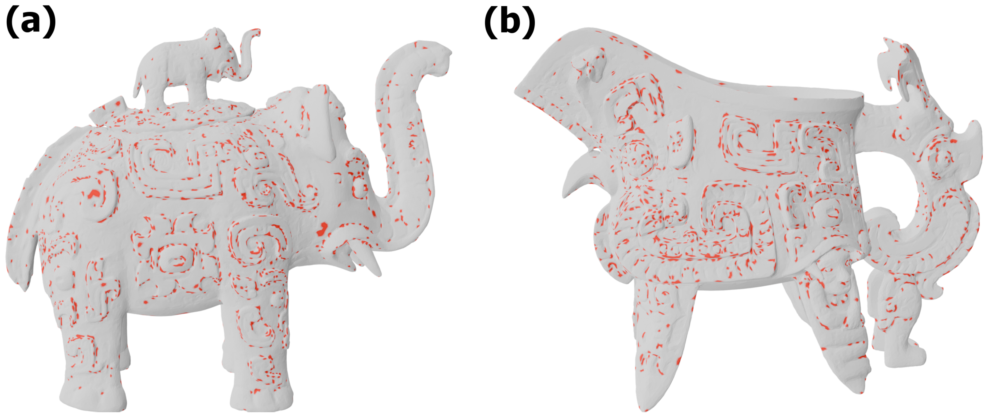
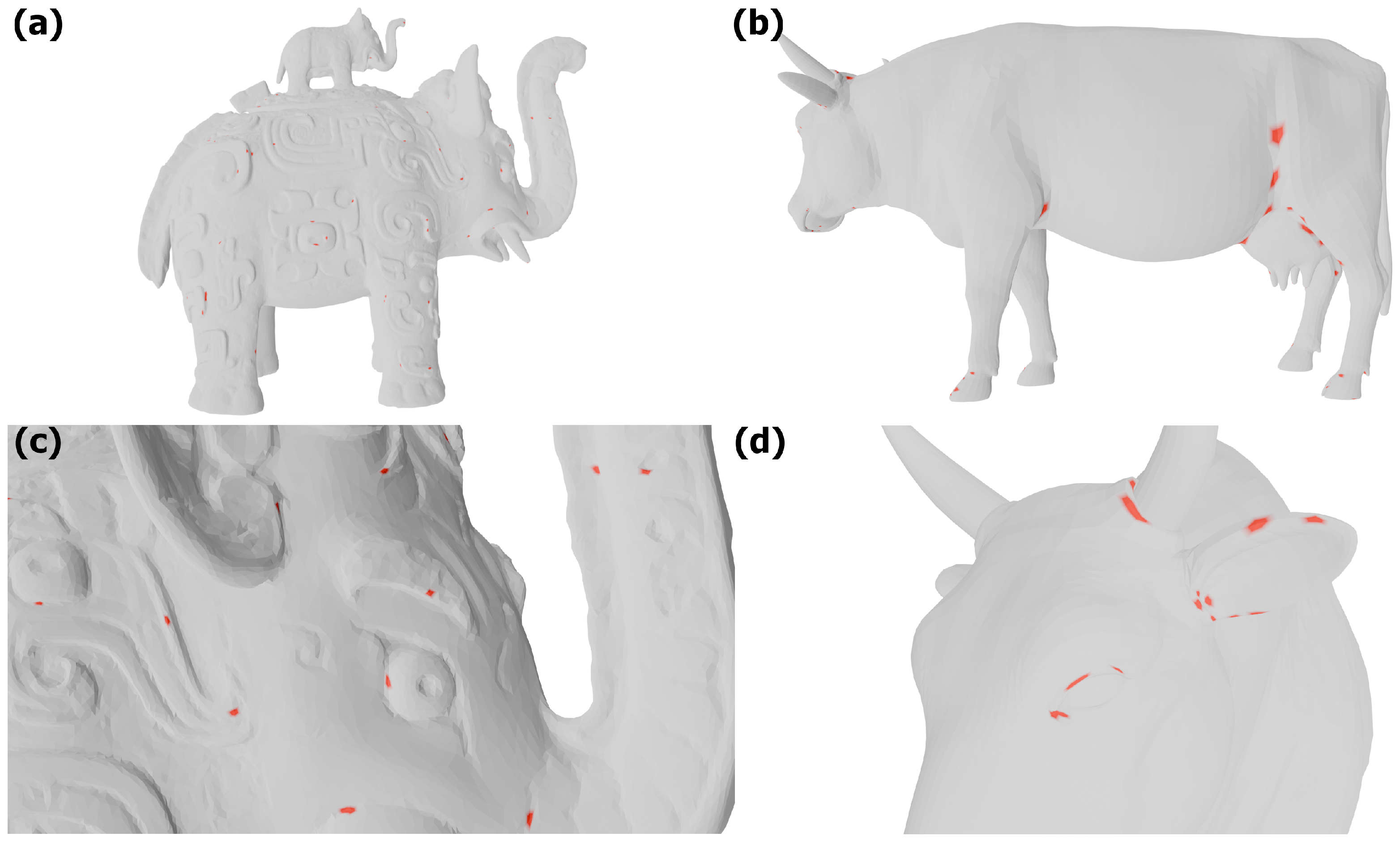
The application of the described Isolation Forest (IF) analysis to 3D models results in the detection of regions characterised by complex and dense geometry. In particular, these include soft edges, areas of curvature, and regions of pronounced mesh folding. Figure 4 and Figure 5 present the results obtained for the elephant and ewer models, which contain approximately 84,000 and 82,000 vertices, respectively. These objects are distinguished by a high number of details and convex elements, which makes the effect clearly visible. Vertices selected on the basis of the feature vector and the IF method are marked in red. To improve readability, a rendering mode was applied in which the triangular fragments adjacent to a vertex are also highlighted in red.

The results of the IF analysis are particularly noteworthy. The vast majority of vertices identified by IF occur in regions where the mesh of the model exhibits strong curvature or folding, whereas flat areas are categorised as normal values. Naturally, some imprecision is present, but the sensitivity of the detection can be adjusted using the contamination parameter, with lower values corresponding to lower sensitivity. Figure 5 presents close-up views of surface fragments with dense geometry. It is clearly visible that steep and more curved regions contain a larger number of vertices marked in red. In addition, Figure 5 also includes a wireframe visualisation of the geometry, which emphasises the complexity of the selected fragments.

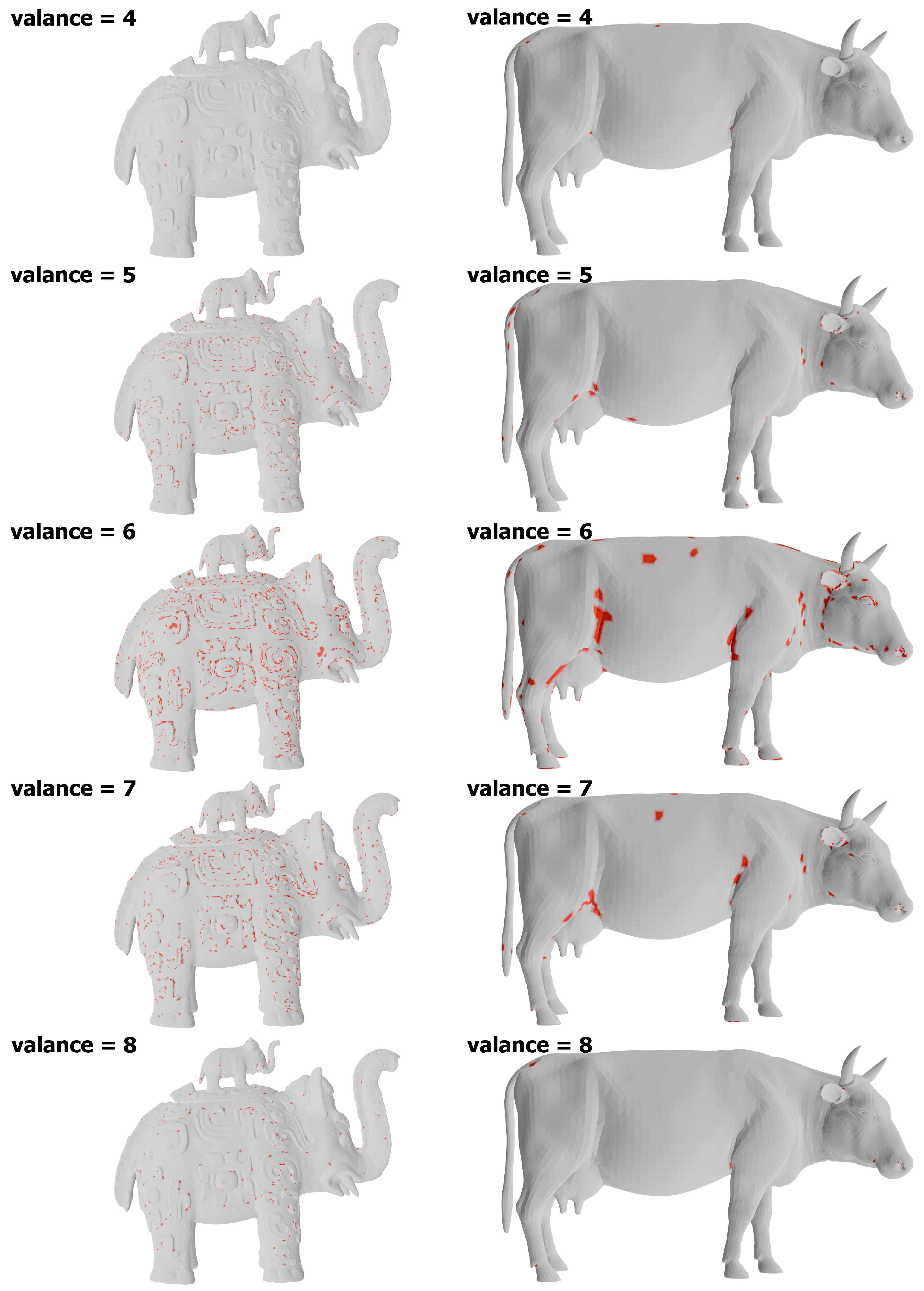
For the sake of completeness, additional experiments were conducted using different values of the valance parameter to thoroughly investigate its influence on the results of the IF analysis. The results are presented in Figure 6, while the information on the number of selected vertices is summarised in

Table 2. The number of vertices selected using Isolation Forest analysis relative to the valance parameter value.

Valance:	4	5	6	7	8
cow	36	257	1085	211	32
elephant	239	2542	4452	2241	384

. An evaluation of the obtained results clearly indicates that a valance value of 6 yields the highest sensitivity of the method and enables the detection of the largest number of vertices belonging to regions with dense and complex geometry.

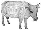
The study also included models with a smaller number of vertices and simpler geometry. Figure 7 shows the vertices selected by Isolation Forest for the pinecone, cow, and vase models. Two different views were generated for each object. The vase model consists of a large number of vertices—approximately 50,000—yet its lateral surface, including the interior and base, essentially forms a flat mesh. The obtained results are consistent with previous observations: edges as well as convex and concave regions were detected, whereas extensive smooth areas were disregarded, even though they are composed of a dense mesh of vertices.

In the case of the cow model (Figure 7), which is considerably less complex than the previous ones and contains around 15,000 vertices, the results are also promising. Among other features, the regions where the limbs are connected were marked, as well as geometric details such as eyelids and corners of the eyes. It should be noted, however, that for models with fewer vertices the detection effect is weaker. A further experiment involved low-poly models—3D graphics models characterised by construction from a small number of polygons.

For low-poly models, the method remains functional, but its usefulness is highly limited. The small number of vertices results in angular geometry with numerous sharp edges, which leads to a highly varied distribution of feature vectors and prevents the formation of clusters of similar elements. In other words, this indicates that nearly all vertices are outliers or anomalies with respect to their various feature vectors (i.e., there are no normal regions), making the IF-based selection less discriminative and, consequently, more random in low-poly models.

Figure 8 presents the results of the IF analysis for two low-poly models: mannequin (≈1500 vertices) and goat (915 vertices). It is worth noting that the marked vertices are not randomly distributed across the entire model but are mostly concentrated in regions where the mesh bends.

Three-dimensional assets can be rendered using various methods. The most common technique is to generate triangles from vertices and subsequently construct the entire geometry from these triangles. In this approach, a square is rendered as two triangles, each defined by three vertices. As a result, a square requires six vertices, two of which are duplicated. An alternative approach relies on a set of unique vertices, where each triangle is defined by an index (an unsigned integer) of a vertex belonging to it. In this case, a square requires four vertices and six indices.

Geometry analysis with the proposed IF method does not support models containing duplicated vertices. In such cases, the method often returns zero vertices or a significantly lower number than expected. Therefore, in order to ensure correct application of Isolation Forest, it is necessary to remove duplicated vertices prior to the start of the procedure. Figure 9a shows the result of the method applied to the astronaut model containing duplicated vertices, whereas Figure 9b presents the same model after the redundant vertices have been removed. The improvement is clearly noticeable.

The original astronaut model consists of 30,837 triangles and approximately 51,000 vertices. The simplified astronaut model contains 30,904 triangles and around 18,000 vertices. This means that approximately 32,000 redundant (duplicated) vertices were removed, while the number of triangles remained almost unchanged. The presence of duplicated vertices is easy to detect: a number of vertices exceeding the number of triangles clearly indicates the existence of duplicates.

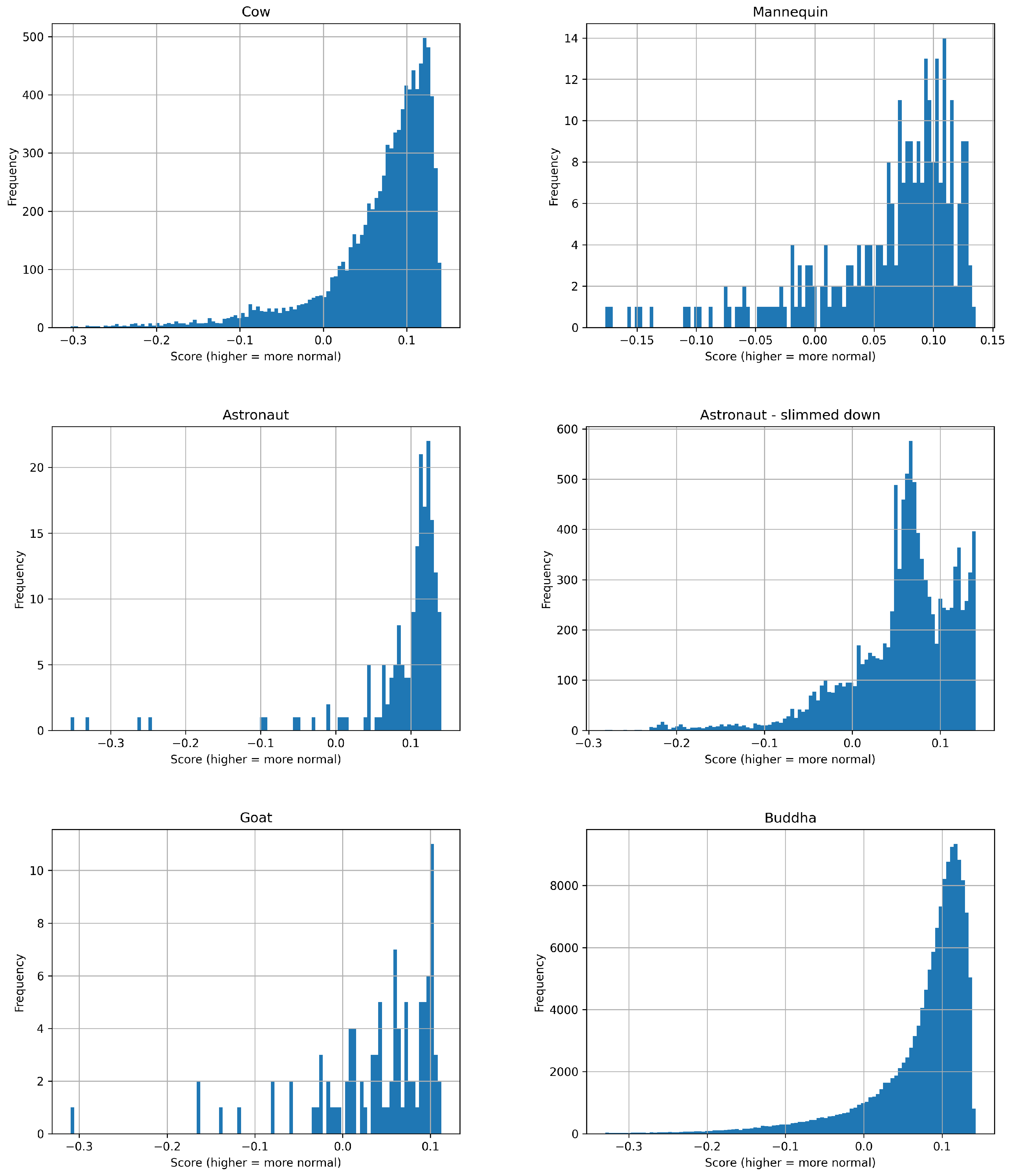
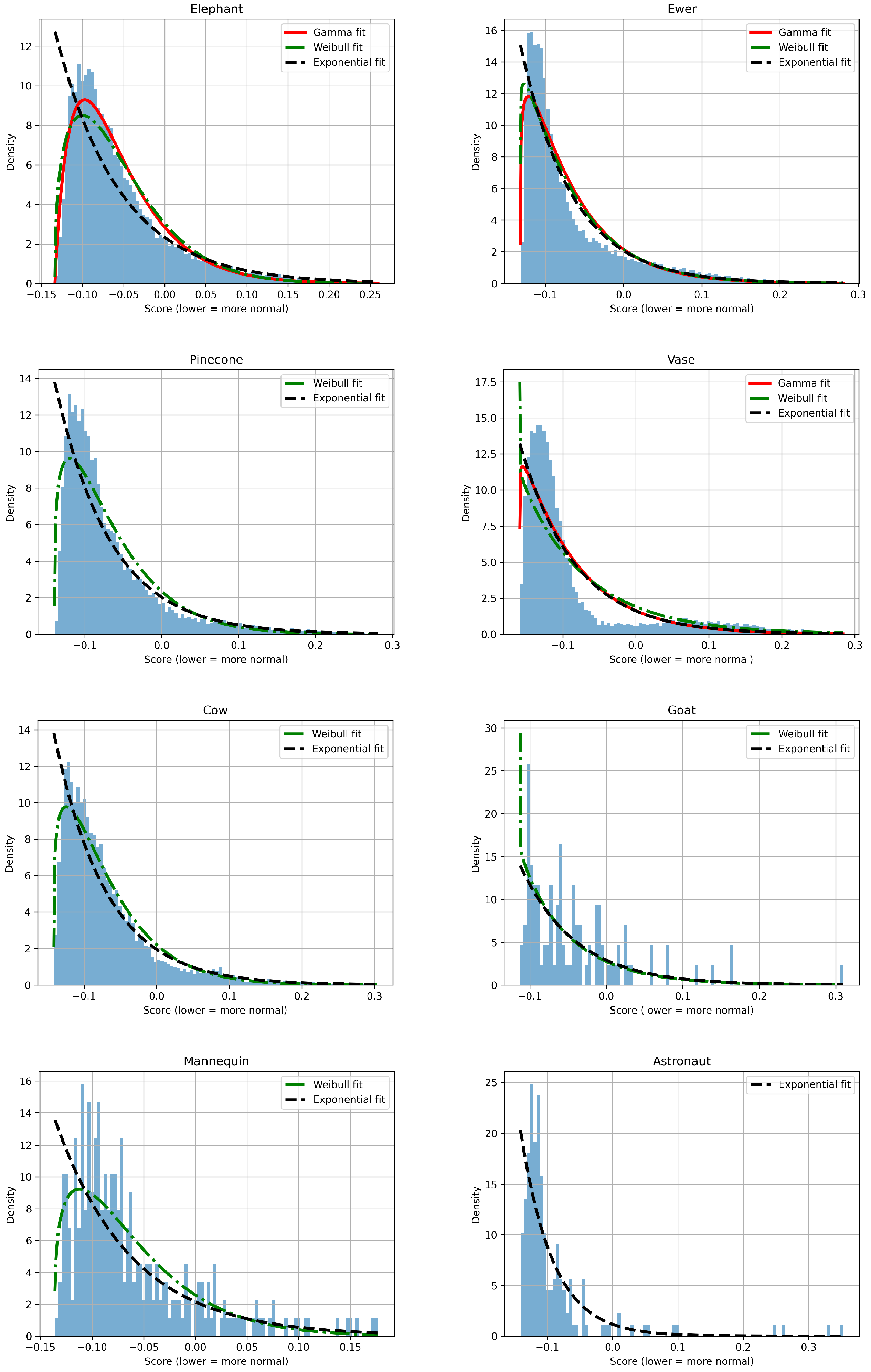
In the conducted study, in addition to vertex selection, histograms of anomaly score were generated for the test models (see Figure 10 and Figure 11). The horizontal axis represents the anomaly score, while the vertical axis shows the number of observations assigned to a given metric value. A higher value indicates a more normal element. Recall that the adopted assumption was $as\left(x\right)<0$ denotes an anomaly, i.e., the vertex is marked in red.

Histogram analysis also yields interesting results. First, for typical 3D models, it can be hypothesized that the anomaly score histogram is characterized by a rise–peak–drop shape. In other words, as the number of vertices increases, the histogram tends to take on this shape. However, an exception is the slimmed-down astronaut model, whose structure resulted from a forced vertex reduction. The number of vertices was reduced in Blender by using the Merge by Distance operation.

To further investigate the implications of vertex reduction on the anomaly score distribution, additional experiments involving models with duplicated vertices were conducted. Recall that models with duplicated vertices represent exceptional cases in the context of our method.

Among the models used in these experiments was the Happy Buddha model from the Stanford 3D Scanning Repository (version: VRipped reconstruction; file name: happy_vrip.ply). A total of 115,031 vertices were removed, resulting in a model consisting of approximately 428,000 vertices, and about 857,000 faces. Due to the massive vertex reduction, the results for the Happy Buddha model were thoroughly analysed. In this case, the histogram exhibits the expected shape (Figure 11), indicating that vertex reduction (with Blender’s Merge by Distance algorithm) does not always directly cause unusual histogram shapes.

After normalising the histograms and applying the transformation $f\left(x\right)=-as\left(x\right)$ (where a lower value indicates a more normal element), the resulting graphs can be approximated by probability and statistical distributions. Figure 12 shows the fit of the Gamma, Weibull, and Exponential distributions. It was not possible to fit all curves to all histograms. It should be emphasized that the conclusions remain valid only under identical conditions to those in the study.

As expected, the histograms (Figure 10 and Figure 11) also indicate that the vast majority of vertices belong to the normal element group. This is as expected since anomalies typically constitute only a small percentage of all observations. The results prove the validity and usefulness of the algorithm: Isolation Forest allows details such as small geometric elements, soft edges, intense mesh folds and areas of pronounced curvature to be detected. These regions constitute a small part of the entire mesh structure, in the same way that anomalies constitute a small part of the entire dataset. All of this confirms the correctness of the reasoning presented regarding the construction of the feature vector and the application of Isolation Forest.

We recommend our method for watermarking 3D scans of historical artefacts, as models obtained in this way typically consist of a large number of vertices [38,39]. Another potential application area is the watermarking of models included in motion capture datasets [40]. The models included in such collections are valuable and often require copyright/licence protection [41].

5. Comparison to Other Solutions

The imperceptibility of modifications is widely regarded as the most desirable property of methods and algorithms in the field of steganography and watermarking. In the case of audio signals or images (two-dimensional signals), the primary objective is to achieve the near-perfect masking of alterations. Signal analysis techniques such as Fast Fourier Transform [42], Discrete Wavelet Transform [43], Singular Value Decomposition [44], and Discrete Cosine Transform [45] are commonly employed to identify signal components that exert minimal influence on overall quality, into which additional information can be embedded.

In 3D model steganography and watermarking, the aforementioned methods exhibit limited applicability due to the specific nature of the data. Consequently, results obtained through Isolation Forest (IF) analysis are highly valuable, as they identify vertices with significant potential for information hiding. Vertices selected using IF are primarily located in regions with dense and complex geometry, such as folds, concavities, or pronounced mesh undulations. Modifications introduced in these areas are less perceptible than alterations to large, flat surface regions of the model [15,16].

In this section, we present the results of metrics computed according to Equations (2)–(4), and compare them with the results reported in other recent studies on 3D model watermarking.

The watermark length was set to 384 bits, which resulted in the modification of 128 vertices. Consequently, the payload size was 48 bytes. Considering the steganographic potential of the method, the payload could be significantly higher. However, it is strongly dependent on the model since a model containing a larger number of vertices allows the IF analysis to detect more of them. According to Table 2, the IF analysis with a valance value of 6 returned 4452 vertices for the elephant model. In this case, the payload could reach 4452 × 3 = 13,356 bits, or even more if additional least significant bits (LSBs) were utilised. However, for the cow model, which is significantly less complex, the method detected only 1085 vertices under the same settings. Hence, the payload limit depends on the number of vertices selected by the IF method, which is directly influenced by the total number of vertices in the model.

The proposed method is blind, meaning that the verification process does not require access to the original model. Moreover, it utilizes a fragile watermark [46]—a type of watermark that is highly sensitive to any modification of the object—in contrast to robust watermarking [47], whose main function is to be resistant to tampering by unauthorised users. In our case, any attempt at unauthorized modification of the model—even a single-bit change—breaks the watermark. This behaviour results from the nature of the HMAC function (BLAKE2), which is designed so that even a one-bit change in the input data produces a completely different output. Therefore, we did not analyse various attack scenarios such as noise addition or cropping attacks. Fragile watermarks are generally used as tools for authentication and integrity verification, rather than for copyright protection.

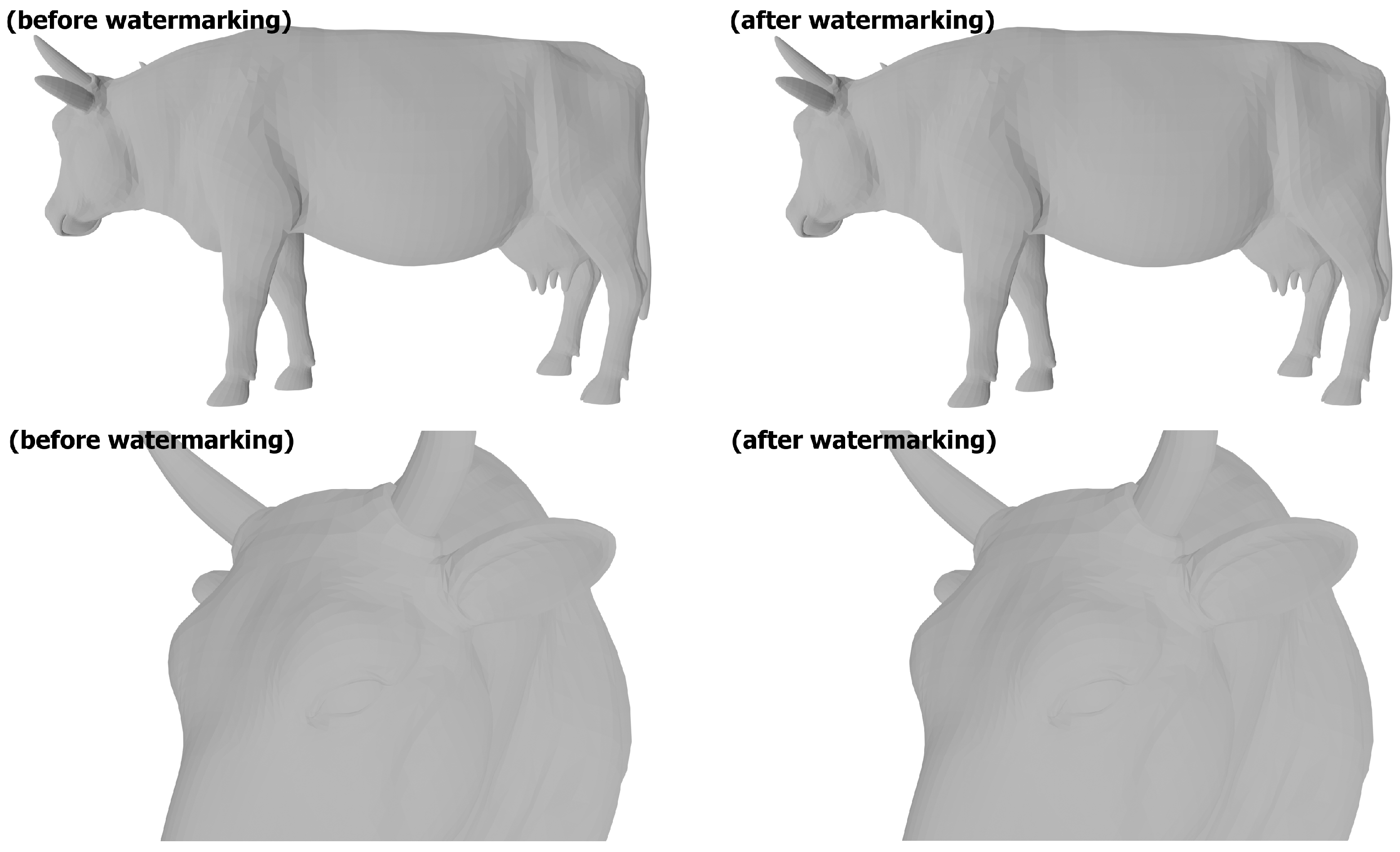
The presented watermarking method demonstrates a high level of imperceptibility of the introduced modifications, owing to the minimal alterations applied to the vertex position coordinate values. Figure 13 illustrates the locations where the watermark bits are embedded, while Figure 14 and Figure 15 compare the models before and after watermark embedding.

Table 3. Summary of the SNR metric (dB) for test models; the higher the score, the better. Values are rounded to the nearest whole number. The term Astronaut* denotes the slimmed-down version of the astronaut model.

Name:	Elephant	Ewer	Vase	Pinecone	Cow	Astronaut*
SNR	172	172	170	171	166	166

shows the Signal-to-Noise Ratio (SNR) values calculated for the watermarked models. Higher SNR values indicate lower levels of distortion introduced into the object. The best results were obtained for the elephant, ewer, vase, and pinecone models. Since these models consist of tens of thousands of vertices, the introduced noise represents a smaller proportion of the whole compared to simpler mesh models, such as cow and astronaut*.

Table 4. Evaluation of the proposed method based on RMSE $\times {10}^{-8}$ metrics; the lower the score, the better. The term Astronaut* denotes the slimmed-down version of the astronaut model.

Name:	Elephant	Ewer	Vase	Pinecone	Cow	Astronaut*
RMSE	0.029	0.034	0.057	0.023	1.110	0.638

presents the Root Mean Square Error (RMSE) values calculated for the watermarked models. Lower RMSE values indicate better performance, as this metric reflects the error between the vertex positions of the original and watermarked models. The best results were obtained for the pinecone, elephant, ewer, and vase models. Although the number of modified vertices in each model was identical (128 vertices were altered), the RMSE metric also depends on the total number of vertices in the mesh (see the denominator in Equation (3)). Consequently, models with larger numbers of vertices achieved the lowest RMSE values.

The final metric used to evaluate the proposed watermarking method is the Hausdorff Distance (HD). The values presented in

Table 5. Evaluation of the proposed method based on HD $\times {10}^{-6}$ metrics; the lower the score, the better. The term Astronaut* denotes the slimmed-down version of the astronaut model.

Name:	Elephant	Ewer	Vase	Pinecone	Cow	Astronaut*
HD	0.017	0.021	0.018	0.009	0.219	0.137

should be interpreted such that lower values indicate better performance. The HD metric measures the difference between two models in terms of dissimilarity. Introducing the same amount of noise into two different objects does not necessarily result in the same level of distortion. This is well illustrated by the pinecone model, which achieved the lowest HD value. Although the pinecone model has fewer vertices than the elephant, ewer, or vase models, its chaotic mesh structure effectively conceals the introduced modifications, thereby reducing their visibility.

In terms of SNR, the proposed method achieves higher values than the methods of Matczuk et al. [30] and Wang et al. [16]. In our study, the cow model, consisting of approximately 15,000 vertices (V) and 30,000 faces (F), achieved an SNR of 166 dB, whereas Wang et al.’s method yielded an SNR of 52 dB for the bunny model, which has around 36,000 V and 70,000 F. Matczuk et al.’s method achieved 169 dB for the pinecone model, while our method returned 171 dB for the same model.

The main difference lies in vertex selection: Matczuk et al. selected vertices randomly—choosing n vertices from the full set, where n depends on the length of the watermark (also represented as a code generated by a hash function). This randomness increases the likelihood that visually prominent vertices in flat areas may be modified. In contrast, our method selects only vertices in regions with complex, dense, and folded geometry. This targeted selection contributes to the slightly higher SNR achieved by our approach.

These results indicate that the proposed method better preserves the model’s quality after watermark embedding.

In terms of RMSE, our results are lower compared to the reference methods, indicating a smaller degree of deviation from the original mesh. Kozieł and Malomuzh [25] reported an RMSE on the order of ${10}^{-4}$ for the pinecone model. El Zein et al. [29] obtained an RMSE on the order of ${10}^{-3}$ for the rabbit model, which consists of approx. 70,000 vertices (V) and 141,000 faces (F). Botta et al. [26] achieved an RMSE of ${10}^{-6}$ for an object comprising approx. 16,000 V and 17,000 faces (F). In Sharma et al. [22], the method produced an RMSE on the order of ${10}^{-3}$ for a model containing approx. 25,000 V and 50,000 F.

The HD metric indicates that our method minimizes geometric deviations between the original and modified models, particularly for objects with irregular, complex mesh structures, such as the pinecone. The combination of Isolation Forest analysis and watermarking enabled the development of a method that achieved an HD value of $2.19\times {10}^{-7}$ for the cow model, which consists of a moderate number of vertices (approximately 15,000). In contrast, Laftah et al. [24] reported an HD on the order of ${10}^{-4}$ for the david-head model (approx. 24,000 V and 47,000 F). Mouhamed et al. [37] obtained ${10}^{-3}$ for the hand model (approx. 37,000 V and 73,000 F). Similarly, the evaluation of the method by Medimegh et al. [23] showed an HD on the order of ${10}^{-3}$ for a model with approx. 12,000 V and 25,000 F.

6. Conclusions

The present paper sets out the potential of utilising Isolation Forest (IF) for the analysis of 3D model geometry and watermarking. The results obtained represent a significant step forward in the exploration of the area of IF applications. The direction of the research is innovative and may serve as a starting point for identifying a new branch of applications for this method. The results covering edge detection, geometry details, areas with complex structures and mesh bends should be considered promising. Furthermore, the research identified interesting properties of anomaly score metric histograms, which can be successfully approximated by Gamma or Weibull distributions.

The evaluation of the proposed watermarking method presented in Section 4, titled Results and Discussion, and comparison of its results with other works included in Section 5, titled Comparison to Other Solutions, indicates its usefulness and superiority in terms of parameters such as imperceptibility and simplicity of operation compared to other solutions.

7. Future Works

The selected vertices obtained using the described method demonstrate significant steganographic potential. In the designated areas, it is possible to conceal information invisibly or to manipulate vertices in such a manner that the edges and bends of the mesh are smoothed out, with the objective of creating flat areas of the mesh. This research direction merits further consideration in the future.

Any meaningful data transformation that allows for obtaining features describing the model can be combined with Isolation Forest (IF). In light of the increasing prevalence of methodologies that amalgamate numerous machine learning models (Ensemble Transfer Learning) [48,49,50], an extension of the proposed concept could entail a more profound examination of the 3D grid through the implementation of IF analysis as a constituent element of a comprehensive process.