Article

A Gradient-Variance Weighting Physics-Informed Neural Network for Solving Integer and Fractional Partial Differential Equations

School of Mathematical Sciences, Inner Mongolia University, Hohhot 010021, China
*
Author to whom correspondence should be addressed.
Appl. Sci. 2025, 15(20), 11137; https://doi.org/10.3390/app152011137
Submission received: 29 September 2025 / Revised: 14 October 2025 / Accepted: 15 October 2025 / Published: 17 October 2025

Abstract

Physics-Informed Neural Networks (PINNs) have emerged as a promising paradigm for solving partial differential equations (PDEs) by embedding physical laws into the learning process. However, standard PINNs often suffer from training instabilities and unbalanced optimization when handling multi-term loss functions, especially in problems involving singular perturbations, fractional operators, or multi-scale behaviors. To address these limitations, we propose a novel gradient variance weighting physics-informed neural network (GVW-PINN), which adaptively adjusts the loss weights based on the variance of gradient magnitudes during training. This mechanism balances the optimization dynamics across different loss terms, thereby enhancing both convergence stability and solution accuracy. We evaluate GVW-PINN on three representative PDE models and numerical experiments demonstrate that GVW-PINN consistently outperforms the conventional PINN in terms of training efficiency, loss convergence, and predictive accuracy. In particular, GVW-PINN achieves smoother and faster loss reduction, reduces relative errors by one to two orders of magnitude, and exhibits superior generalization to unseen domains. The proposed framework provides a robust and flexible strategy for applying PINNs to a wide range of integer- and fractional-order PDEs, highlighting its potential for advancing data-driven scientific computing in complex physical systems.

1. Introduction

Partial Differential Equations (PDEs) form the mathematical basis for modeling and analyzing a wide range of physical, biological, and engineering phenomena [1]. They provide a unifying framework for describing how quantities such as temperature, concentration, pressure, or electromagnetic fields evolve under spatial and temporal variations. Classical numerical solvers, such as finite difference [2], finite element [3], and spectral methods [4], have achieved remarkable success over the past decades, enabling accurate simulation of complex processes in areas such as fluid dynamics, structural mechanics, quantum physics, and biomedical engineering. However, the rapid growth in the demand for simulating systems with high-dimensional state spaces, irregular geometries, or multiscale structures has revealed intrinsic limitations of these conventional approaches [5,6]. In particular, fractional-order operators introduce non-locality and singularity, dramatically increasing computational complexity and memory requirements [7,8]. As a result, classical solvers often exhibit prohibitively high costs, poor scalability, or degraded stability when applied to these challenging PDEs.
In recent years, machine-learning-based methods have emerged as promising alternatives for addressing these limitations. Neural networks, with their universal function approximation capabilities, offer flexible representations for high-dimensional solution spaces that are difficult to handle with grid-based methods [9]. Among these, Physics-Informed Neural Networks (PINNs) have attracted considerable Attention [10], as they incorporate governing differential equations, boundary conditions, and initial conditions directly into the optimization objective.This formulation allows the learning process to be guided by underlying physical laws rather than relying solely on data-driven fitting, thus reducing the dependence on large labeled datasets [11,12,13]. PINNs have demonstrated encouraging success across a wide range of applications, including turbulent and laminar fluid dynamics, wave propagation and scattering in acoustics and electro-magnetics, nonlinear heat conduction in complex media, and anomalous transport modeled by fractional diffusion [14,15,16]. The flexibility of PINNs lies in their ability to seamlessly incorporate complex geometrical domains and various forms of PDEs, while their efficiency stems from avoiding expensive mesh generation and numerical integration procedures. Despite these advantages, PINNs are not without significant challenges. A primary difficulty arises when applying them to stiff ODEs, highly oscillatory multiscale problems, or fractional-order models involving integral or nonlocal operators [17,18]. In such cases, training becomes unstable and convergence may stagnate or lead to inaccurate solutions. The root cause is often attributed to the imbalance among different loss components, namely the PDE residuals, boundary conditions, and initial conditions [19]. If one component dominates, the optimization process may bias the network toward satisfying only part of the problem constraints while neglecting others, ultimately reducing accuracy and generalization capacity. Furthermore, the optimization landscape of PINNs is typically highly non-convex, and gradient magnitudes across different terms may vary by orders of magnitude, aggravating the imbalance. While several strategies such as adaptive loss weighting, gradient normalization, curriculum training, and residual-based adaptive sampling have been proposed, these techniques tend to be problem-dependent, require manual tuning of hyper-parameters, and often lack robustness across different PDE families [20,21,22,23,24].
To overcome these limitations, we propose in this work a Gradient Variance Weighting (GVW) strategy that adaptively balances different loss terms in the PINN framework. The key idea is to monitor the variance of the magnitudes of the gradients during the training process and dynamically assign weights so that no single term overwhelms the optimization process. In this way, GVW provides an automatic and principled mechanism to ensure stable convergence across diverse PDE types, without requiring problem-specific tuning. We integrate GVW into the standard PINN architecture and systematically validate the approach on three representative problems: (i) the heat conduction equation, representing a prototypical parabolic PDE; (ii) the two-dimensional Helmholtz equation with acoustic scattering, which is highly oscillatory and involves complex boundary conditions; (iii) a time-fractional diffusion equation with Riemann–Liouville derivatives, capturing memory effects and anomalous transport. Numerical experiments demonstrate that GVW-PINN significantly enhances training stability, accuracy, and robustness compared to baseline PINN formulations. These findings highlight GVW-PINN as a general and effective strategy for solving both integer-order and fractional-order PDEs, providing a new pathway for reliable neural network–based scientific computing.
The structure of this paper is organized as follows. Section 2 introduces the proposed methodology, detailing the GVW-PINN framework and how it differs from the standard PINN paradigm. Section 3 presents the experimental setups and results on representative integer-order and fractional-order PDE problems. Section 4 discusses the performance, mechanism, and limitations of GVW-PINN, while Section 5 concludes the work and outlines future research directions.

2. Methodology

In this section, we will present the methodological framework of the study. We first introduce the standard PINN, including its formulation and training strategy, and then describe the proposed GVW-PINN, which adaptively balances the loss terms based on gradient variance. This methodological foundation serves as the basis for the comparative experiments conducted on the following representative PDE problems.

2.1. Methodology of the Standard Physics-Informed Neural Network

Physics-Informed Neural Networks (PINNs) are a class of deep learning models that incorporate physical laws, expressed in the form of partial differential equations (PDEs), into the training process of neural networks. We consider a general PDE defined over a spatial domain Ω R d and temporal domain [ 0 , T ] :
N [ u ( x , t ) ] = f ( x , t ) , ( x , t ) Ω × [ 0 , T ] ,
I [ u ( x , t ) ] = u ( x , 0 ) = u 0 ( x ) , x Ω ,
B [ u ( x , t ) ] = g ( x , t ) , ( x , t ) Ω × [ 0 , T ] ,
where N [ · ] denotes the differential operator defining the governing PDE, I [ · ] represents the operator enforcing the initial condition at t = 0 , and B [ · ] means the operator enforcing the boundary condition in Ω . In fact, the neural network serves as a universal approximator for the unknown solution u(x,t) to the underlying PDE. It is typically implemented as a fully connected feedforward neural network (FNN), composed of three main parts: the input layer, one or more hidden layers, and the output layer. Each of these layers plays a specific and essential role in representing the solution function. In the PINN framework, the governing PDE, along with the initial and boundary conditions, is embedded into the loss function of the neural network, and the overall loss function is defined as The overall loss function of the PINN is defined as
L ( θ ) = λ p d e L p d e ( θ ) + λ i c L i c ( θ ) + λ b c L b c ( θ ) ,
where L p d e , L i c , and L b c denote the residual losses associated with the PDE, the initial condition and the boundary condition, respectively, and λ p d e , λ i c , λ b c are the corresponding penalty weights. The parameter set θ = { W ( l ) , b ( l ) } l = 1 M represents all trainable weights and biases of the neural network. Specifically, the loss terms are formulated as
L p d e ( θ ) = 1 N p d e j = 1 N p d e | N [ u θ ( x p d e j , t p d e j ) ] f ( x p d e j , t p d e j ) | 2 ,
L i c ( θ ) = 1 N i c j = 1 N i c | I [ u θ ( x i c j , 0 ) ] u 0 ( x i c j ) | 2 ,
L b c ( θ ) = 1 N b c j = 1 N b c | B [ u θ ( x b c j , t b c j ) ] g ( x b c j , t b c j ) | 2 ,
where { ( x p d e j , t p d e j ) } j = 1 N p d e , { x i c j } j = 1 N i c , and { ( x b c j , t b c j ) } j = 1 N b c are collocation points sampled in the interior domain, on the initial surface, and on the boundary, respectively.
In summary, the key of the PINN method is to determine suitable neural network parameters θ such that the network prediction u θ ( x , t ) closely approximates the exact solution u ( x , t ) . This is achieved by minimizing a composite loss function that embeds the residuals of the PDE, initial, and boundary conditions, enforcing these constraints through unified residual minimization.

2.2. Methodology of the Gradient-Variance Weighting Physics-Informed Neural Network

In traditional Physics-Informed Neural Networks, the total objective function is typically composed of multiple sub-losses that correspond to distinct physical constraints, such as the partial differential equation residual, boundary conditions, and initial conditions. These sub-losses are often weighted equally or with manually tuned constants. Such weighting schemes frequently lead to imbalanced training, where certain sub-tasks dominate the optimization process while others are neglected, resulting in slow convergence and reduced accuracy. To mitigate this issue, we propose a Gradient-Variance Weighting (GVW) strategy. It dynamically adjusts the weight of each sub-loss based not only on its gradient magnitude but also on the temporal variability of that gradient throughout the training process.

2.2.1. Theoretical Formulation

In GVW-PINN, let the total loss function be composed of N sub-loss terms:
L total = i = 1 N ω ˜ i L i ,
where ω ˜ i is the adaptive normalized weight for the i-th loss component. The gradient of the i-th loss term L i with respect to the network parameters θ can be expressed as
θ L i ( θ ) = L i ( θ ) θ = 2 N i j = 1 N i O i [ u θ ( x j , t j ) ] y j O i [ u θ ( x j , t j ) ] θ ,
where O i [ · ] denotes the corresponding operator (e.g., N , I , or B ), y j is the target value, and u θ ( x j , t j ) is the network output. In each training epoch t { 1 , 2 , , k } , we compute the Euclidean ( 2 ) norm of the gradient of each loss term:
g i ( t ) : = θ L i ( θ ( t ) ) 2 = 2 N i j = 1 N i O i [ u θ ( t ) ( x j , t j ) ] y j O i [ u θ ( t ) ( x j , t j ) ] θ 2 ,
to assess the temporal stability of each loss term, we set a window size T = 0.05 k (i.e., 5% of total epochs) and compute the variance of gradient norms over the recent T epochs:
σ i 2 ( t ) : = Var { g i ( t T + 1 ) , , g i ( t ) } , t T ,
we then define an intermediate weight that balances both the current gradient magnitude and its variance:
w i ( t ) = g i ( t ) σ i 2 ( t ) + ε ,
where ε > 0 is a small constant introduced for numerical stability. To obtain the final adaptive weights, we normalize across all loss components:
w ˜ i ( t ) = w i ( t ) j = 1 N w j ( t ) ,
and after substituting into the overall loss function yields the final dynamically weighted formulation
L total ( t ) = i = 1 N ω i ( t ) L i ( t ) .

2.2.2. Two-Phase Weighting Strategy

To ensure statistical reliability, we adopt a two-phase strategy:
  • Warm-up phase ( t < T ):
    Equal weights are assigned to all sub-losses:
    w ˜ i ( t ) = 1 N ,
    where N is the number of loss terms.
  • GVW phase ( t T ):
    The full GVW theoretical formulation is applied as described above.
Compared with the traditional PINN framework, the proposed GVW-PINN offers several significant advantages:
1.
When the gradient of a particular loss component becomes very small (indicating near convergence) or exhibits high gradient variance (reflecting instability), its corresponding weight is automatically reduced, thereby mitigating potential negative effects on the overall training process.
2.
The method enables self-balanced optimization across different tasks (e.g., PDE residual, boundary, and initial conditions) without the need for manual tuning of loss weights.
3.
It simultaneously promotes convergence by emphasizing informative gradients and enhances training stability by suppressing variance-dominated components, leading to improved robustness and generalization across a broad spectrum of PDE problems.
Figure 1 illustrates the schematic diagram of the proposed GVW-PINN architecture.

3. Experimental Results

To evaluate the effectiveness of the proposed Gradient Variance Weighting Physics-Informed Neural Network (GVW-PINN), we conducted a series of experiments on three representative classes of partial differential equations. These include a heat conduction equation, a two-dimensional Helmholtz scattering problem with a rigid circular obstacle, and a time-fractional diffusion equation involving the Riemann–Liouville derivative. The availability of exact analytical solutions for these PDEs provides a reliable reference against which the performance of the improved algorithm can be systematically evaluated. By examining convergence behavior and prediction accuracy across these problems, we aim to demonstrate how the gradient-variance weighting strategy enhances both the stability and generalization capability of PINNs in solving challenging integer- and fractional-order PDEs.

3.1. Heat Conduction Equation

The heat conduction equation serves as a basic validation case to demonstrate the reliability of the proposed PINN framework prior to addressing more challenging PDEs. We consider the following initial-boundary value problem for the heat conduction equation:
u t = α 2 u x 2 , x ( 0 , 1 ) , t ( 0 , 1 ] , u ( x , 0 ) = sin ( π x ) , x [ 0 , 1 ] , u ( 0 , t ) = u ( 1 , t ) = 0 , t [ 0 , 1 ] ,
here, u ( x , t ) denotes the temperature distribution over a spatio-temporal domain, and the thermal diffusivity is taken as α = 0.2 . The initial condition is sinusoidal, and the boundary conditions are homogeneous Dirichlet type, representing a rod held at zero temperature at both ends. This problem admits an exact analytical solution given by [25]
u ( x , t ) = e α π 2 t sin ( π x ) ,
which decays exponentially in time. This analytical solution will be used to evaluate the accuracy of the neural network predictions during training and testing.
To approximate the solution of the heat equation, we construct a fully connected feedforward neural network (FNN) consisting of an input layer, three hidden layers with 32 neurons each, and a single-neuron output layer, resulting in a total of five layers. For both the PINN and GVW-PINN methods, the network takes the spatio-temporal coordinate pair ( x , t ) [ 0 , 1 ] × [ 0 , 1 ] as input. The activation function after each hidden layer is the hyperbolic tangent (tanh), which is known for its smoothness and suitability for representing continuous physical fields. The final output layer produces the network’s approximation of the scalar solution of the PDE. The network is implemented in PyTorch 2.4.1 using the torch.nn.Module framework, where all layers are dynamically created with nn.ModuleList, and the forward pass is performed by applying linear transformations followed by the Tanh activation function at each hidden layer.
To train the neural network, three types of points are sampled from the spatio-temporal domain ( x , t ) [ 0 , 1 ] × [ 0 , 1 ] : interior points for enforcing the PDE residual, initial points for imposing the initial condition, and boundary points for satisfying the boundary conditions. A total of 1200 interior points are generated within the domain ( 0 , 1 ) × ( 0 , 1 ) to minimize the residual of the governing partial differential equation. These points are sampled using a space-filling strategy, such as Latin Hypercube Sampling, to ensure uniform coverage of the domain and avoid clustering. For enforcing the initial condition u ( x , 0 ) = sin ( π x ) , 200 points are sampled along the initial time slice t = 0 , with spatial coordinates x [ 0 , 1 ] drawn from a uniform distribution. To impose the homogeneous Dirichlet boundary conditions u ( 0 , t ) = u ( 1 , t ) = 0 , 150 points are generated along the spatial boundaries at x = 0 and x = 1 , with temporal coordinates t [ 0 , 1 ] uniformly sampled. Together, these points provide sufficient constraints to guide the network in approximating the PDE solution throughout the entire spatio-temporal domain. All sampled points are kept fixed throughout the training process. The combination of interior, initial, and boundary samples enables the network to learn a physically consistent solution that satisfies both the differential operator and the associated initial-boundary conditions.
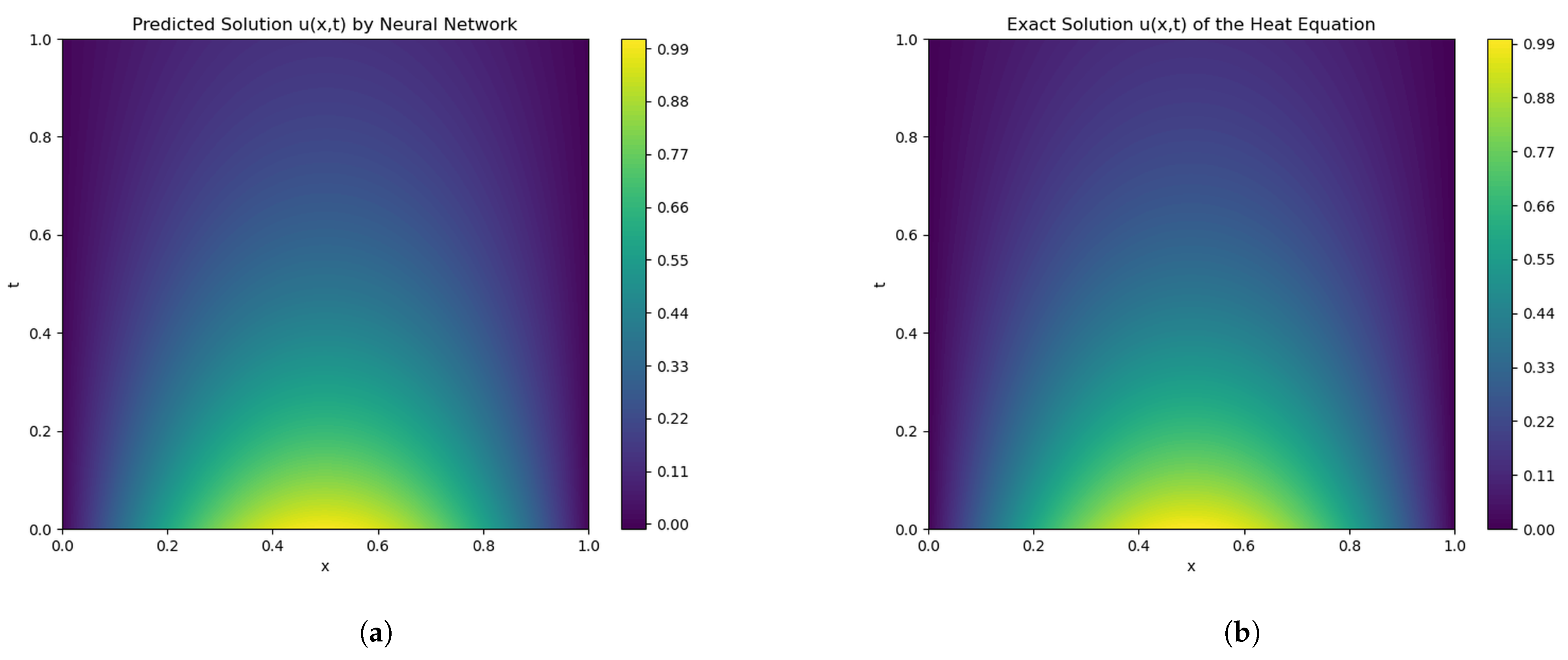
Figure 2 depicts the spatio-temporal solution u ( x , t ) over the entire domain, comparing the GVW-PINN prediction directly with the analytical solution. The visualization demonstrates that GVW-PINN accurately captures the global structure of the solution, without noticeable phase shifts or spurious oscillations.
Figure 3 presents cross-sectional views of the predicted and reference solutions at three representative time instants (t = 0.25, 0.50, and 0.75), illustrating the temporal evolution of the solution as captured by the two methods. The results indicate that while the baseline PINN shows noticeable degradation in accuracy at later times, the GVW-PINN maintains close agreement with the reference solution, highlighting its superior capability in capturing the temporal dynamics.
Figure 4 illustrates the convergence behavior of PINN and GVW-PINN during training. The GVW-PINN exhibits a smoother and faster decay of the total loss, reaching a lower and more stable value within fewer epochs. This demonstrates the enhanced stability and improved optimization dynamics afforded by the gradient-variance weighting strategy. In contrast, the standard PINN converges more slowly and shows oscillatory fluctuations, indicating less efficient loss reduction and difficulties in balancing the multiple loss components.

3.2. Two-Dimensional Acoustic Scattering Problem Governed by the Helmholtz Equation

We consider a two-dimensional acoustic scattering problem governed by the Helmholtz equation with a sound-hard circular obstacle [26]. The computational domain is defined as a square region Ω outer = [ π , π ] 2 , with a circular obstacle D = { ( x , y ) x 2 + y 2 R 2 } , where R = π / 4 . The effective computational domain is the annular region Ω = Ω outer D . The complex-valued wave field u ( x , y ) = u real ( x , y ) + i u imag ( x , y ) satisfies the Helmholtz equation:
Δ u + k 0 2 u = 0 , in Ω ,
where k 0 = 2 is the wave number and Δ is the Laplace operator. On the circular boundary D , we impose a Neumann condition that simulates a sound-hard boundary. Let the incident wave be u inc ( x , y ) = e i k 0 x , the boundary condition then becomes
u n = u inc n , on D ,
which, after separating real and imaginary parts, gives
u real n = Re u inc n , u imag n = Im u inc n ,
on the outer boundary Ω outer , a first-order absorbing boundary condition is applied:
u n + i k 0 u = 0 , on Ω outer ,
which, after separating real and imaginary parts, gives
u real n k 0 u imag = 0 , u imag n + k 0 u real = 0 .
The total acoustic field is expressed as the superposition of the incident wave and the scattered field, i.e., u ( x , y ) = u inc ( x , y ) + u sc ( x , y ) . The scattered wave u sc is constructed using a Fourier expansion in polar coordinates, where the radial dependence of each mode is represented by Bessel functions for the interior domain and Hankel functions for the exterior radiating field [27,28]. The Neumann boundary condition on the circular obstacle determines the coefficients of each mode, yielding a classical analytical solution that serves as a benchmark for validating the performance of PINNs and GVW-PINNs.
We employ a fully-connected feedforward neural network to approximate the real and imaginary components of the complex acoustic wave field. The network takes the spatial coordinates ( x , y ) as input and outputs the two solution components, Re ( u ) and Im ( u ) . It consists of an input layer with 2 neurons, four hidden layers with 120 neurons each using the hyperbolic tangent (tanh) activation, and an output layer with 2 neurons. All weights are initialized using the Glorot uniform initializer. Collocation points are generated within the computational domain and on its boundaries using Latin Hypercube Sampling, with 3200 interior points capturing the acoustic oscillations and 1400 boundary points uniformly distributed along both the circular obstacle and the outer square boundary. These points remain fixed during training to provide consistent enforcement of the PDE residuals and boundary conditions. The network is trained using a two-stage optimization procedure: first with the Adam optimizer at a learning rate of 10 3 , followed by L-BFGS for further refinement. The loss function includes contributions from the PDE residuals and all boundary conditions, with equal weighting for the standard PINN; in the case of GVW-PINN, gradient-variance weighting is applied to dynamically balance the loss components.
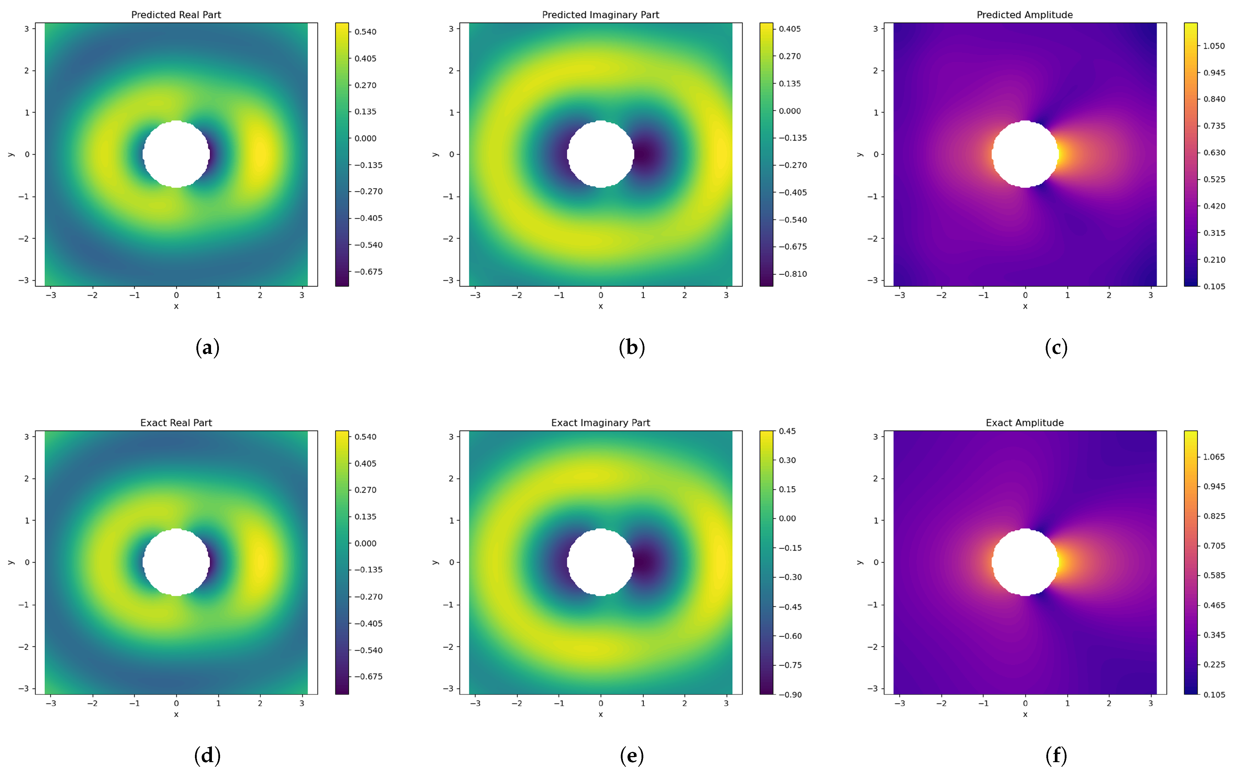
Figure 5 presents the density plot of the solution of the two-dimensional Helmholtz equation with a sound-hard circular obstacle, where both the predicted results from GVW-PINN and the exact analytical solutions are shown. GVW-PINN achieves a close match with the analytical solution, with minimal visual differences. The predictions are stable across the real, imaginary, and amplitude fields, indicating enhanced robustness. Overall, the improved algorithm ensures high fidelity in representing both the field components and amplitude of the scattered wave, making it reliable for solving Helmholtz-type wave propagation problems with complex boundary conditions.
Figure 6 shows cross-sectional comparisons at fixed x values ( 2 ,   3 ). The standard PINN fails to accurately capture the real and imaginary components, particularly near the boundaries, exhibiting noticeable deviations, minor oscillations, and phase shifts, which are common failures in high-frequency wave simulations. In contrast, the GVW-PINN predictions align almost perfectly with the analytical solution, producing smooth and stable numerical results across the entire domain. This demonstrates that the gradient-variance weighting mechanism significantly enhances accuracy and training stability.
Figure 7 presents the loss curves during training for the two methods. GVW-PINN exhibits a faster decline in loss during the early stages, indicating more efficient optimization. Its real and imaginary loss components decrease smoothly and reach low values within fewer epochs. By the end of training, GVW-PINN achieves a lower final loss compared to the standard PINN. These results demonstrate not only the faster convergence of GVW-PINN but also its superior final accuracy.

3.3. Time-Fractional Diffusion Equation with Riemann–Liouville Derivatives

u ( x , t ) t + D 0 + α + D 1 α u ( x , t ) = f ( x , t ) , ( x , t ) ( 0 , 1 ) × ( 0 , 1 ] , u ( x , 0 ) = x 3 ( 1 x ) 3 , x [ 0 , 1 ] , u ( 0 , t ) = u ( 1 , t ) = 0 , t [ 0 , 1 ] ,
here, D 0 + α and D 1 α denote the left- and right-sided Riemann–Liouville fractional derivatives of order α , and f ( x , t ) is the source term. We employ the method of manufactured solutions by prescribing a smooth analytical solution with suitable boundary behavior [16,29,30], and substituting it into the governing equation to obtain the corresponding source term. The analytical solution is given by
u ( x , t ) = e t x 3 ( 1 x ) 3 .
We adopt a fully-connected neural network with four hidden layers of 35 neurons each, whose output is transformed to exactly satisfy the boundary and initial conditions, allowing the network to learn the residual of the fractional diffusion equation. The spatio-temporal domain ( x , t ) ( 0 , 1 ) × ( 0 , 1 ) is discretized into collocation points, boundary points, initial condition points, and auxiliary points for the numerical approximation of the Riemann–Liouville fractional derivatives. Specifically, 4000 collocation points cover the interior to represent the PDE residual, 500 boundary points impose the Dirichlet conditions, and points along t = 0 enforce the initial condition. A fixed mesh of 800 auxiliary points is used to support the evaluation of the fractional derivatives. This strategy ensures adequate coverage of both the physical constraints and the nonlocal effects inherent to the fractional operators.
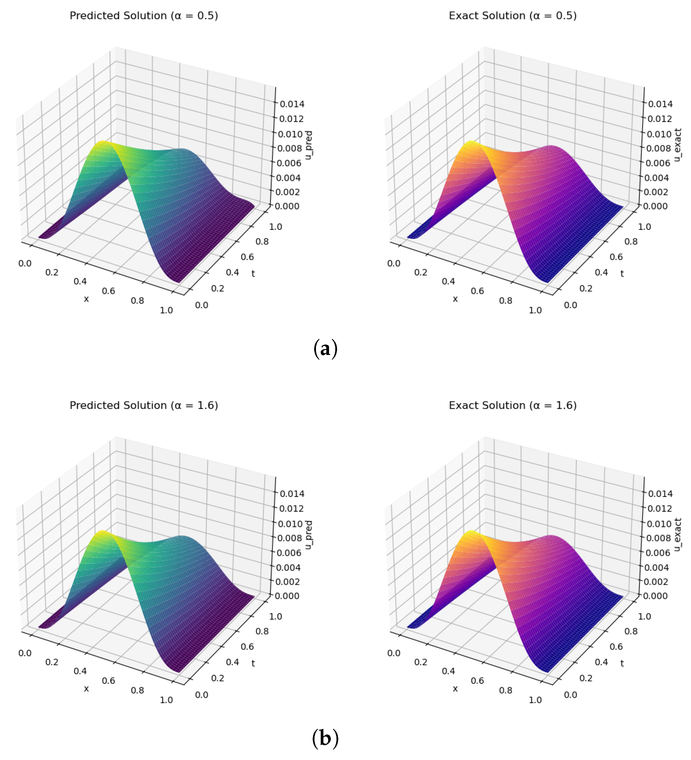
Figure 8 illustrates the performance of the proposed GVW-PINN method in solving the time-fractional diffusion equation under different fractional orders α . The predicted surfaces demonstrate a close agreement with the analytical solutions across the tested values of α . The surfaces are smooth, the peak amplitudes align accurately with the exact solutions, and the temporal decay rate is well preserved. This indicates that the gradient variance weighting strategy enhances both the accuracy and stability of the training process, particularly in challenging fractional-order regimes.
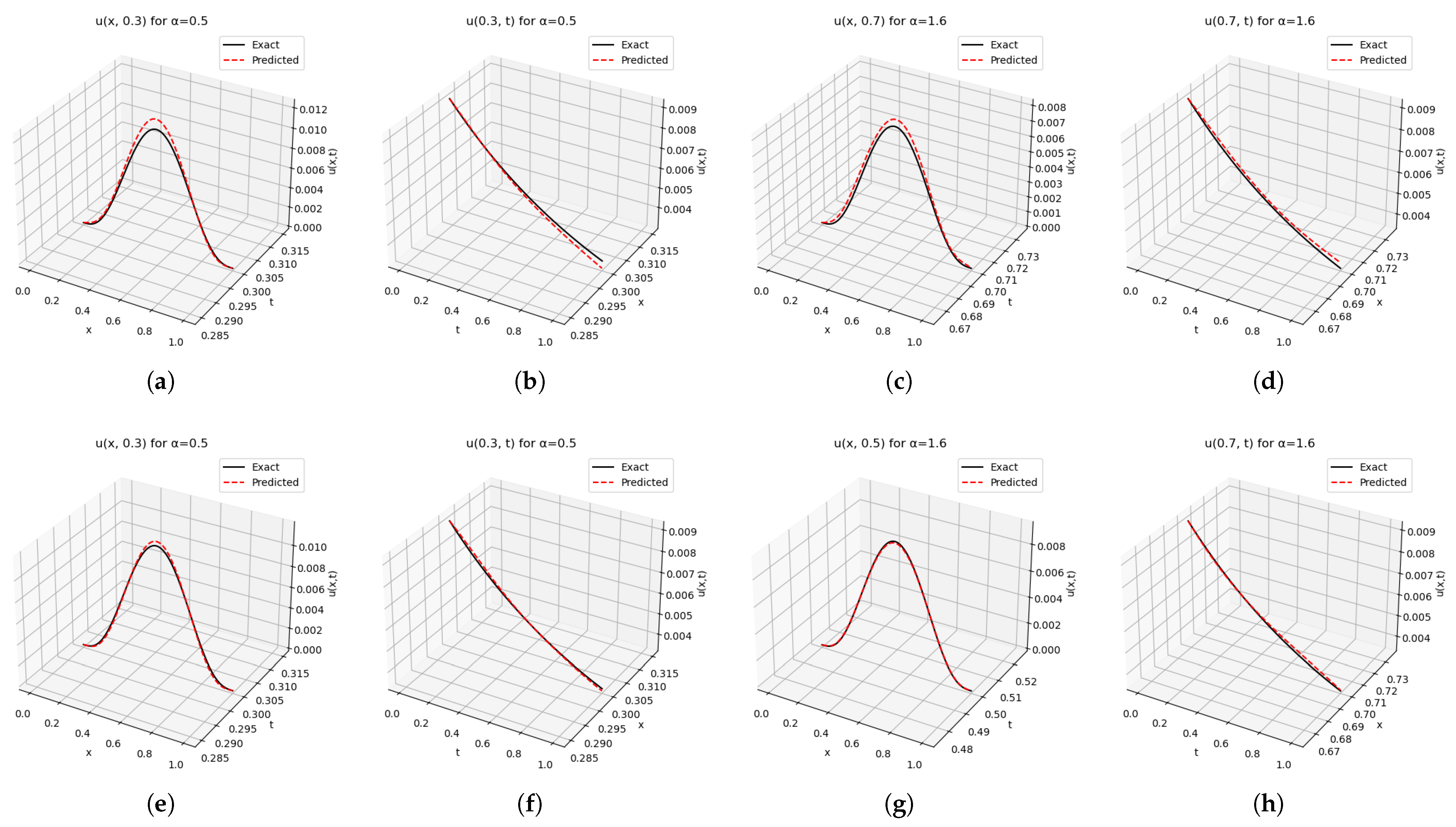
Figure 9 provides a detailed validation of the predicted solutions by comparing one-dimensional slices of the solution surface at fixed spatial and temporal positions. For the standard PINN, the predicted curves capture the overall trend but deviate from the exact solutions, particularly around the peak regions where amplitudes are overestimated. These discrepancies become more pronounced with α = 1.6 . In contrast, GVW-PINN achieves nearly perfect agreement with the analytical solutions across the tested cases. The red dashed lines almost overlap with the black solid lines, indicating that gradient variance weighting effectively balances the training dynamics and enhances the model’s generalization.
Figure 10 shows the training loss evolution for the standard PINN and the proposed GVW-PINN across different fractional orders. While the standard PINN initially reduces the loss, it soon exhibits slow convergence, and frequent stagnation at relatively high loss values, particularly for higher fractional orders ( α = 1.6 ,   1.8 ), indicating a clear inability to capture the dynamics of stronger fractional effects. In contrast, GVW-PINN demonstrates faster and smoother loss decay for all α values, achieving reductions up to two orders of magnitude compared to PINN, and reflecting more stable optimization and better generalization. Overall, GVW-PINN converges within fewer epochs, reaches consistently lower final loss magnitudes, and maintains robust performance across all tested fractional orders, significantly enhancing both accuracy and training stability for fractional diffusion problems with pronounced nonlocal effects.
In addition, to quantitatively assess the predictive accuracy, we employ the relative L 2 error defined as u pred u exact 2 u exact 2 , which measures the discrepancy between the predicted and exact solutions, and the results in Table 1 clearly demonstrate that GVW-PINN consistently enhances solution accuracy while providing more reliable and robust performance across a wide range of problem settings including integer and fractional-order systems.

4. Discussion

In this section, we critically analyze the proposed GVW-PINN framework by highlighting its performance improvements, examining the underlying mechanism of gradient variance weighting, and acknowledging its limitations. The discussion aims to position GVW-PINN within the broader context of PINN methodologies while clarifying its contributions and potential avenues for future development.

4.1. Performance Improvements and Robustness

The proposed GVW-PINN framework exhibits clear improvements over the standard PINN in terms of convergence speed, accuracy, stability, and generalization. In particular, the method proves highly effective for challenging scenarios such as oscillatory Helmholtz equations, PDEs with complex boundary conditions, and fractional-order diffusion problems, where traditional PINNs often struggle to achieve reliable accuracy. These results underscore the robustness of GVW-PINN in handling both integer-order and fractional-order systems.

4.2. Mechanism of Gradient Variance Weighting

The central advantage of GVW-PINN lies in its gradient-variance weighting mechanism, which dynamically balances multiple loss terms based on the evolving distribution of their gradients. This approach differs fundamentally from existing adaptive sampling or residual-based balancing strategies, which mainly target point selection or residual magnitudes [31]. By leveraging information embedded in gradient dynamics, GVW provides a more general and problem-independent solution to the intrinsic imbalance of loss components, thereby enabling more stable and effective training across diverse PDE classes.

4.3. Limitations and Future Work

Nevertheless, certain limitations should be acknowledged. The additional computation required for gradient statistics introduces extra training cost, which could become significant for large-scale models. Moreover, the adaptability of GVW-PINN to high-dimensional PDEs and highly irregular domains remains to be systematically evaluated. Finally, the performance of the method may depend on the choice of hyperparameters such as the statistical window size, suggesting that further research is needed to optimize these aspects.

5. Conclusions

This study introduced GVW-PINN, a physics-informed neural network enhanced with a gradient-variance weighting strategy. The framework establishes a principled way to mitigate loss imbalance, resulting in faster convergence and more reliable training across diverse PDE settings. Its demonstrated effectiveness on both integer-order and fractional-order problems highlights its versatility and potential as a broadly applicable tool for physics-informed learning. Beyond these achievements, the proposed approach not only delivers practical improvements but also contributes to strengthening the theoretical foundations of adaptive weighting strategies in neural networks for scientific computing. By explicitly leveraging gradient variance to guide the balance of multiple loss components, GVW-PINN provides a more systematic and generalizable perspective that can inspire further methodological developments in this area.
Prospectively, GVW-PINN holds the potential to be extended to higher-dimensional PDEs, large-scale multiphysics systems, and problems defined on irregular or evolving domains. Furthermore, it can be integrated with complementary advances such as adaptive sampling schemes, domain decomposition methods, and emerging neural architectures, thereby offering a flexible and powerful paradigm for addressing increasingly complex scientific and engineering challenges.

Author Contributions

Conceptualization, L.Z. and Z.D.; methodology, L.Z.; software, L.Z.; validation, L.Z. and Z.D.; formal analysis, L.Z.; investigation, L.Z.; resources, L.Z., Q.L. and Z.D.; data curation, L.Z. and L.Y.; writing—original draft preparation, L.Z.; writing—review and editing, L.Z., Q.L. and R.Z.; visualization, L.Z. and Z.D.; supervision, Q.L., R.Z. and Z.D.; project administration, Z.D.; funding acquisition, Z.D. All authors have read and agreed to the published version of the manuscript.

Funding

Authors acknowledge financial support provided by the National Natural Science Foundation of China (Nos. 11902165, 12272188, 12102205 and 12262025), the National Science Foundation for Distinguished Young Scholars of the Inner Mongolia Autonomous Region of China (No. 2023JQ16), the Program for Young Talents of Science and Technology in Universities of Inner Mongolia Autonomous Region (NJYT23098), the Scientific Startin and the Innovative Research Team in Universities of Inner Mongolia Autonomous Region of China (No. NMGIRT2208), and the Natural Science Foundation of Inner Mongolia Autonomous Region (Nos. 2025ZDLH007 and 2025QN01014). The APC was funded by the Program for Young Talents of Science and Technology in Universities of Inner Mongolia Autonomous Region (NJYT23098).

Institutional Review Board Statement

Not applicable.

Informed Consent Statement

Not applicable.

Data Availability Statement

All original contributions of this study are contained within the article; additional information is available from the corresponding author upon request.

Conflicts of Interest

The authors declare no conflicts of interest.

References

  1. Evans, L.C. Partial Differential Equations, 2nd ed.; American Mathematical Society: Providence, RI, USA, 2010. [Google Scholar]
  2. LeVeque, R.J. Finite Difference Methods for Ordinary and Partial Differential Equations: Steady-State and Time-Dependent Problems; SIAM: Philadelphia, PA, USA, 2007. [Google Scholar]
  3. Lehrenfeld, C.; Olshanskii, M.A. An Eulerian finite element method for PDEs in time-dependent domains. ESAIM Math. Model. Numer. Anal. 2019, 53, 585–614. [Google Scholar] [CrossRef]
  4. Bueno-Orovio, A.; Pérez-García, V.M.; Fenton, F.H. Spectral methods for partial differential equations in irregular domains: The spectral smoothed boundary method. SIAM J. Sci. Comput. 2006, 28, 886–900. [Google Scholar] [CrossRef]
  5. Alzahrani, H.; Turkiyyah, G.; Knio, O.; Keyes, D. Space-fractional diffusion with variable order and diffusivity: Discretization and direct solution strategies. J. Comput. Phys. 2021, 435, 110162. [Google Scholar] [CrossRef]
  6. Efendiev, Y.; Galvis, J.; Hou, T.Y. Generalized multiscale finite element methods. J. Comput. Phys. 2013, 251, 116–135. [Google Scholar] [CrossRef]
  7. Garrappa, R. Neglecting nonlocality leads to unreliable numerical methods for fractional differential equations. Commun. Nonlinear Sci. Numer. Simul. 2019, 70, 302–306. [Google Scholar] [CrossRef]
  8. Moghaddam, B.P.; Babaei, A.; Dabiri, A.; Galhano, A. Fractional stochastic partial differential equations: Numerical advances and practical applications—A state of the art review. Symmetry 2024, 16, 563. [Google Scholar] [CrossRef]
  9. Goodfellow, I.; Bengio, Y.; Courville, A. Deep Learning; MIT Press: Cambridge, MA, USA, 2016. [Google Scholar]
  10. Raissi, M.; Perdikaris, P.; Karniadakis, G.E. Physics-informed neural networks: A deep learning framework for solving forward and inverse problems involving nonlinear PDEs. J. Comput. Phys. 2019, 378, 686–707. [Google Scholar] [CrossRef]
  11. Cuomo, S.; Di Cola, V.S.; Giampaolo, F.; Rozza, G.; Raissi, M.; Piccialli, F. Scientific machine learning through physics-informed neural networks: Where we are and what’s next. J. Sci. Comput. 2022, 92, 88. [Google Scholar] [CrossRef]
  12. Lu, L.; Meng, X.; Mao, Z.; Karniadakis, G.E. DeepXDE: A deep learning library for solving differential equations. SIAM Rev. 2021, 63, 208–228. [Google Scholar] [CrossRef]
  13. Karniadakis, G.E.; Kevrekidis, I.G.; Lu, L.; Perdikaris, P.; Wang, S.; Yang, L. Physics-informed machine learning. Nat. Rev. Phys. 2021, 3, 422–440. [Google Scholar] [CrossRef]
  14. Jin, X.; Cai, S.; Li, H.; Karniadakis, G.E. NSFnets (Navier–Stokes Flow nets): Physics-informed neural networks for the incompressible Navier–Stokes equations. J. Comput. Phys. 2021, 426, 109951. [Google Scholar] [CrossRef]
  15. Song, C.; Alkhalifah, T.; Waheed, U.B. Solving the frequency-domain acoustic VTI wave equation using PINNs. Geophys. J. Int. 2021, 227, 1928–1947. [Google Scholar] [CrossRef]
  16. Pang, G.; Lu, L.; Karniadakis, G.E. fPINNs: Fractional Physics-Informed Neural Networks. SIAM J. Sci. Comput. 2019, 41, A2603–A2626. [Google Scholar] [CrossRef]
  17. Weng, Y.; Zhou, D. Multiscale Physics-Informed Neural Networks for Stiff Chemical Kinetics. J. Phys. Chem. A 2022, 126, 8534–8543. [Google Scholar] [CrossRef]
  18. Mustajab, A.H.; Lyu, H.; Rizvi, Z.; Wuttke, F. Physics-Informed Neural Networks for High-Frequency and Multi-Scale Problems Using Transfer Learning. Appl. Sci. 2024, 14, 3204. [Google Scholar] [CrossRef]
  19. Wang, J.; Xiao, X.; Feng, X.; Xu, H.; Hui, X. An improved physics-informed neural network with adaptive weighting and mixed differentiation for solving the incompressible Navier–Stokes equations. Nonlinear Dyn. 2024, 111, 2345–2365. [Google Scholar] [CrossRef]
  20. Hou, J.; Li, Y.; Ying, S. Enhancing PINNs for solving PDEs via adaptive collocation point movement and adaptive loss weighting. Nonlinear Dyn. 2023, 111, 15233–15261. [Google Scholar] [CrossRef]
  21. Mao, Z.; Meng, X. Physics-informed neural networks with residual/gradient-based adaptive sampling methods for solving partial differential equations with sharp solutions. Appl. Math. Mech. (Engl. Ed.) 2023, 44, 1069–1084. [Google Scholar] [CrossRef]
  22. Wang, S.; Teng, Y.; Perdikaris, P. Self-adaptive loss balanced physics-informed neural networks (lbPINNs). Neurocomputing 2022, 496, 11–34. [Google Scholar] [CrossRef]
  23. Gao, B.; Yao, R.; Li, Y. Physics-informed neural networks with adaptive loss weighting algorithm for solving partial differential equations (APINNs). Comput. Math. Appl. 2025, 181, 216–227. [Google Scholar]
  24. Wang, J.; Gao, H.; Sun, H. A simple remedy for failure modes in physics-informed neural networks. Neural Netw. 2025, 183, 106963. [Google Scholar] [CrossRef]
  25. Crank, J. The Mathematics of Diffusion, 2nd ed.; Oxford University Press: Oxford, UK, 1975. [Google Scholar]
  26. Bouche, D.; Hong, Y.; Jung, C.-Y. Asymptotic analysis of the scattering problem for the Helmholtz equation with high wave numbers. Discret. Contin. Dyn. Syst. 2017, 37, 2581–2602. [Google Scholar] [CrossRef]
  27. Moiola, A. Scattering of Time-Harmonic Acoustic Waves: Helmholtz Equation; MNAPDE2022; University of Pavia: Pavia, Italy, 2022. [Google Scholar]
  28. Spence, E.A. Wavenumber-explicit bounds in time-harmonic acoustic scattering. SIAM J. Math. Anal. 2014, 46, 2987–3024. [Google Scholar] [CrossRef]
  29. Saadat, M.; Mangal, D.; Jamali, S. UniFIDES: Universal fractional integro-differential equations solver. Comput. Math. Appl. 2022, 103, 23–45. [Google Scholar] [CrossRef]
  30. Wang, S.; Zhang, H.; Jiang, X. Fractional Physics-informed Neural Networks for Time-fractional Phase Field Models. Nonlinear Dyn. 2022, 110, 2715–2739. [Google Scholar] [CrossRef]
  31. Wu, C.; Zhu, M.; Tan, Q.; Kartha, Y.; Lu, L. A Comprehensive Study of Non-Adaptive and Residual-Based Adaptive Sampling for Physics-Informed Neural Networks. Comput. Methods Appl. Mech. Eng. 2022, 396, 115100. [Google Scholar] [CrossRef]
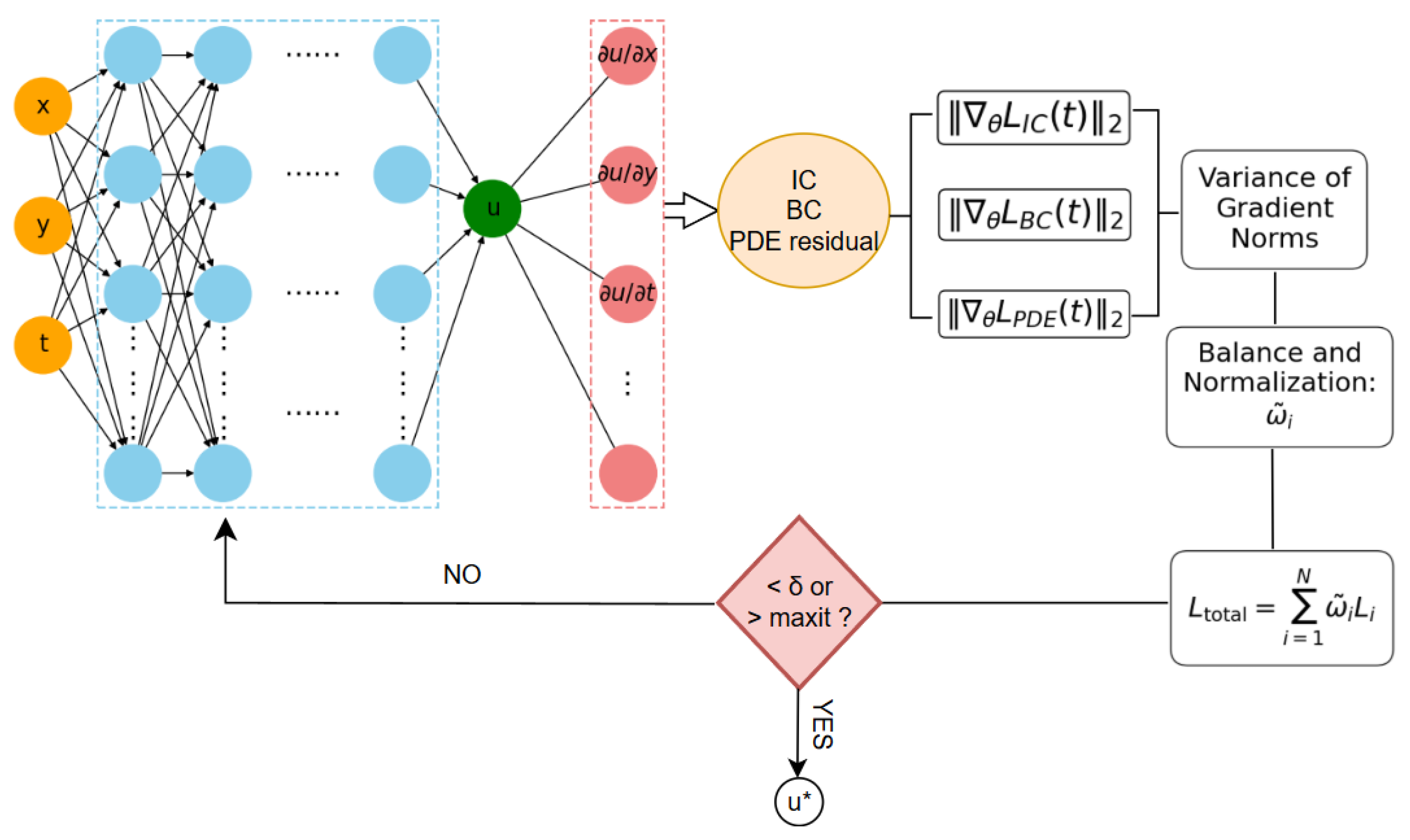
Figure 1. The schematic diagram of GVW-PINN architecture.
Applsci 15 11137 g001
Figure 2. Heat conduction equation based on the GVW-PINN algorithm. (a) Predicted solution u ( x , t ) by GVW-PINN. (b) Exact solution u ( x , t ) of the equation.
Applsci 15 11137 g002
Figure 3. Cross-sectional comparisons of the predicted solutions at three representative time instants: (ac) corresponding to the standard PINN, and (df) corresponding to the GVW-PINN. The GVW-PINN demonstrates enhanced stability and better agreement with the analytical reference across all time slices.
Applsci 15 11137 g003aApplsci 15 11137 g003b
Figure 4. Training loss curves for the heat conduction equation. (a) Loss curve of the standard PINN. (b) Loss curve of the GVW-PINN.
Applsci 15 11137 g004
Figure 5. Density plots of the acoustic field components for the two-dimensional Helmholtz equation with a sound-hard circular obstacle. (ac) show the predicted real part, imaginary part, and amplitude obtained by GVW-PINN, while (df) present the corresponding exact analytical solutions.
Applsci 15 11137 g005
Figure 6. Cross-sectional comparison of the predicted and exact solutions at fixed x values. (a,b) Results obtained by the standard PINNs. (c,d) Results obtained by the GVW-PINN.
Applsci 15 11137 g006aApplsci 15 11137 g006b
Figure 7. Training loss curves for the Helmholtz equation. (a) Loss curve of the standard PINN. (b) Loss curve of the GVW-PINN.
Applsci 15 11137 g007
Figure 8. Predicted solutions of the time-fractional diffusion equation obtained by GVW-PINN compared with the exact solutions for different fractional orders α . (a) α = 0.5 . (b) α = 1.6 .
Applsci 15 11137 g008
Figure 9. Cross-sectional comparisons of the predicted and exact solutions of the one-dimensional time-fractional diffusion equation at different spatial-temporal points for fractional order α = 0.5 , 1.6 . The solid black lines denote the exact solutions, while the red dashed lines represent the predictions. (ad) corresponding to the standard PINN. (eh) corresponding to the GVW-PINN.
Applsci 15 11137 g009
Figure 10. Training loss curves for the fractional diffusion equation. (a) Loss curve of the standard PINN. (b) Loss curve of the GVW-PINN.
Applsci 15 11137 g010
Table 1. Relative L 2 errors of PINN and GVW-PINN for different PDEs.
ProblemFractional Order α PINNGVW-PINN
Heat conduction equation 3.593 × 10 2 6.439 × 10 4
Helmholtz equation 4.375 × 10 1 7.419 × 10 2
Fractional diffusion equation 1.6 1.736 × 10 1 6.672 × 10 3
0.5 3.318 × 10 1 8.491 × 10 3
Disclaimer/Publisher’s Note: The statements, opinions and data contained in all publications are solely those of the individual author(s) and contributor(s) and not of MDPI and/or the editor(s). MDPI and/or the editor(s) disclaim responsibility for any injury to people or property resulting from any ideas, methods, instructions or products referred to in the content.