Uncovering Causal Factors Influencing Hog Prices: A Deep Granger Causality Inference Model for Multivariate Time Series Dynamics

Abstract

The swine industry is vital to economic stability and household welfare in China and worldwide but remains highly vulnerable to price volatility driven by multiple factors. Capturing the underlying mechanisms of hog price formation is particularly challenging, as conventional models often fail to represent its nonlinear structures and complex multivariate causal dependencies. This study proposes a Deep Granger Causality Inference (DGCI) model that integrates deep learning with causal inference to identify the key driving factors of hog price dynamics. The DGCI model contains a Feature Reconstruction Module (FRM) and a Granger Causality Module (GCM). The FRM integrates a Variational Autoencoder (VAE) with a Transformer to capture latent temporal representations of multivariate variables. Meanwhile, the GCM quantifies nonlinear Granger causality strength by systematically excluding features to measure their causal impact on hog price. Furthermore, this study proposes the Causal Feature Importance (CFI) metric, which jointly evaluates reconstruction fidelity and causal strength to identify key determinants. To evaluate the model performance, this study utilizes a real-world hog dataset from China. The results demonstrate considerable gains, with DGCI decreasing MSE by 17.59% to 39.22% and MSPE by 32.35% to 54.90% relative to baseline models. The DGCI model highlights pork price, piglet cost, and slaughter volume as the primary determinants of hog price, with CFI values of 1.5216, 1.4451, and 1.4266, respectively. By advancing understanding of the causal drivers of price volatility, this study contributes to informed decision-making, enhanced food security, and the sustainable development of the swine industry. Moreover, as a generalizable methodology, the proposed framework can be broadly applied to analyze the influencing factors of other agricultural and livestock products.

1. Introduction

The swine industry in China is not only a cornerstone of the national economy but also directly linked to farmers’ livelihoods and residents’ living costs. Reported by the National Bureau of Statistics of China (NBS) (http://www.stats.gov.cn/, accessed on 13 October 2025), pork is the dominant source of animal protein, accounting for 77.46% of per capita meat consumption in 2024 [1]. Meanwhile, fluctuations in pork prices exert a strong influence on the Consumer Price Index (CPI), typically contributing 2–2.5% [2], thereby affecting the purchasing power of households. According to the Ministry of Agriculture and Rural Affairs (MARA) (https://english.moa.gov.cn/, accessed on 13 October 2025), there are 19.18 million pig farms in operation in 2022, and the industry provides significant employment opportunities. For pig farmers, hog production is often the primary source of income, and profit margins are highly sensitive to feed costs and market prices. Thus, stable hog prices are essential for safeguarding both household welfare and rural livelihoods.

However, China’s swine market has been marked by substantial volatility in recent years [3]. According to the MARA, pork production declined from 54.04 million tons in 2018 to 42.55 million tons in 2019, a year-on-year decrease of 21.3% caused by the outbreak of African Swine Fever (ASF). During this period, pork prices surged to nearly 50 CNY/kg [4]. Such extreme fluctuations impose dual risks: farmers face severe operational losses when production costs exceed market returns, while consumers endure significant increases in food expenditure. The Chinese government has introduced multiple policy measures, such as pork reserve releases, subsidies for breeding sows, and adjustments to grain and feed import tariffs, aiming to smooth price cycles and stabilize market expectations. Nevertheless, persistent volatility in hog prices continues to disrupt production stability, reduce farmers’ income, undermine rural welfare, and affect macroeconomic stability.

Fluctuations in the hog market stem from a complex interplay of multiple factors [5,6]. Several key elements contribute to pig price volatility [7], including substitute supply and demand dynamics, production efficiency improvements, and technological advancements. Existing research categorizes the factors influencing pig price fluctuations into endogenous and exogenous variables [8]. Endogenous factors are intrinsic to the production system and pig supply chain, encompassing feed costs [9], the number of breeding sows [10], piglet price [11], total pig inventory [12], and pig-to-grain price ratios [13]. In contrast, exogenous factors represent external shocks that impact agricultural prices, such as shifts in consumer demand [14], disease outbreaks [15], and policy interventions [16]. Identifying these determinants is crucial because it enables governments to improve early warning systems, optimize reserve management, and design more effective policy interventions. For farmers, knowledge of the driving factors provides a scientific basis for production planning and investment decisions, which helps to reduce losses and improve resilience.

Existing research investigating the factors influencing hog prices primarily employs three main methodological approaches: econometric models, causality studies, and machine learning (ML) models. Econometric models, such as Vector Autoregression (VAR) [17] and Error Correction Models (ECMs) [18], are widely applied in this domain. These models typically analyze the direct intensity and direction of specific factors’ impacts on hog prices and characterize dynamic transmission pathways using techniques such as impulse response analysis and variance decomposition. For causality and time-lag analysis, numerous studies [19] utilize the Granger causality test [20] to establish statistical causal relationships between breeding sow populations and hog prices, determining the time lag for production capacity transmission to prices through lag order analysis within VAR frameworks. More recently, ML-based algorithms such as Support Vector Regression (SVR) [21] and Extreme Gradient Boosting (XGBoost) [22] have been introduced for hog price forecasting. These studies leverage the built-in feature importance metrics, such as Gini impurity reduction or permutation-based importance, to identify key influencing factors. However, existing methodologies exhibit significant limitations. Traditional econometric models (e.g., VAR) are often predicated on linear assumptions, thereby limiting their ability to capture complex interactions and nonlinear dependencies between variables.

The causal inference [23] aims to uncover structural cause–effect relationships, often requiring controlled experiments, instrumental variables, or causal graphical models to establish mechanism-based explanations [24]. While Granger causality [20] has been widely adopted in the analysis of agricultural and economic systems, it is essential to recognize its conceptual distinction from traditional causal inference. Granger causality is fundamentally a statistical notion of causality based on predictive relationships: if the inclusion of past values of one variable significantly improves the forecast accuracy of another variable, the former is said to Granger-cause the latter. However, this notion of causality does not necessarily imply the existence of an underlying causal mechanism. Despite its usefulness, traditional Granger causality methods are primarily linear and pairwise, thereby lacking the ability to capture nonlinear dependencies, multivariate interactions, and indirect causal chains. Moreover, Granger causality often assumes stationarity and model adequacy, conditions that are rarely satisfied in agricultural contexts characterized by high-dimensional, noisy, and non-stationary data. These limitations hinder its ability to fully characterize the intricate causal structure of hog price dynamics.

To address the limitations of existing research, this study proposes an innovative Deep Granger Causality Inference (DGCI) model specifically designed to uncover nonlinear causal relationships among multivariate variables. The DGCI architecture comprises two core modules: a Feature Reconstruction Module (FRM) and a Granger Causality Module (GCM). The Feature Reconstruction Module leverages a hybrid architecture combining Variational Autoencoders (VAE) [25] and Transformers [26] to construct powerful nonlinear mappings between multivariate time-series features. The VAE component learns low-dimensional latent representations of high-dimensional hog market data, effectively capturing complex interdependencies and underlying generative mechanisms among features. Meanwhile, Transformers, with their self-attention mechanism, provide superior capability for modeling dynamic interactions and temporal dependencies across variables. The Granger Causality Module quantifies whether a feature Granger-causes the target variable (hog price) and estimates the strength of its causal influence. We exclude specific features and investigate the resultant changes in prediction error for the target variable. Furthermore, we define a novel Causal Feature Importance (CFI) metric that integrates feature reconstruction quality with Granger-causal strength, thereby providing a measure more closely aligned with the causal notion of driving force in the Granger sense.

The DGCI model thus provides a robust theoretical foundation and comprehensive technical framework for analyzing intricate causal relationships within hog market dynamics. Beyond the specific context of the Chinese hog market, the DGCI framework is designed as a generalizable methodology, allowing direct adaptation to other agricultural commodities and even non-agricultural markets. The contribution of this study is as follows:

• We propose the Deep Granger Causality Inference (DGCI) framework, a deep learning model designed to systematically discover the core factors influencing hog prices.
• We develop a feature reconstruction module integrating VAE and Transformer architectures to extract spatiotemporal representations from multivariate inputs. A Granger Causality Module is proposed to quantify multivariate nonlinear Granger causal effects.
• We propose the CFI metric that jointly quantifies representation fidelity and causal impact, providing causally grounded interpretability for multivariate time series drivers.
• Through extensive experiments, the results demonstrate that the proposed DGCI model, benchmarked against Granger causality and correlation-based feature selection, outperforms state-of-the-art baselines. The pork price, piglet cost, and slaughter volume are identified as the key determinants of hog prices.

The rest of this paper is organized as follows: Section 2 provides a brief review on the hog price prediction problem and Granger Causality Inference methods. Section 3 introduces the proposed DGCI method in detail. Section 4 analyzes the experimental results. Finally, the conclusion is drawn in Section 5.

2. Related Works

2.1. Hog Price Prediction

Research pertaining to hog price forecasting methodologies can be broadly categorized into two paradigms: traditional statistical models and machine learning (ML)-based approaches.

Initial investigations predominantly utilized statistical techniques, including AutoRegressive Integrated Moving Average (ARIMA) [27], Vector AutoRegression (VAR) [28], and Exponential Smoothing (ETS) [29]. However, hog price volatility is subject to multifaceted influences, encompassing epidemic outbreaks, policy interventions, market dynamics, and breeding costs [30,31]. The complex interplay among these determinants induces pronounced volatility, manifesting intricate multivariate variation patterns [1]. These traditional approaches, however, remain constrained by linearity assumptions and static correlation analyses, limiting their capacity to capture complex feature interactions. Consequently, the limitations of traditional approaches necessitate more sophisticated methodologies capable of effectively modeling the underlying dynamics of price fluctuations.

Concurrent advancement of Artificial Intelligence (AI) technologies and a substantial increase in relevant data within the hog industry have stimulated extensive research employing machine learning (ML) and deep learning (DL) for price forecasting [32]. To address underlying feature dynamics, ML-based hog price prediction models have gained traction, utilizing methods like Support Vector Regression (SVR) [21], Extreme Gradient Boosting (XGBoost) [22], and Classification and Regression Trees (CART) [33]. To further address complex multivariate dependencies, various DL architectures have been implemented. These include Long Short-Term Memory networks (LSTM) [34] and Transformer architectures [35,36]. Complementary studies [14,37] have systematically identified key determinants spanning supply, demand, macroeconomic conditions, and international market linkages.

Nevertheless, significant challenges remain. Data from the hog industry are characterized by high dimensionality, nonlinear dynamics, and pronounced lag effects, which are poorly handled by traditional statistical methods. Most existing models emphasize predictive accuracy at the expense of causal interpretability, limiting the ability to identify the root drivers of price fluctuations. Moreover, the inherent lag structure of agricultural markets means that drivers influence outcomes with delays, necessitating explicit modeling of temporal dependencies for reliable inference.

2.2. Granger Causality Inference

Traditional causal inference, in contrast, seeks to uncover the true causal mechanisms that govern the relationships between variables [24]. Traditional causal inference aims to distinguish correlation from causation by explicitly addressing issues such as confounding, selection bias, and counterfactual reasoning. Establishing true causality often requires controlled experiments (e.g., randomized controlled trials) or quasi-experimental designs (e.g., instrumental variables, regression discontinuity, or difference-in-differences methods). The goal is to determine not merely whether one variable predicts another, but whether intervening on one variable will reliably produce changes in another.

Granger causality, originally proposed by [20], is a statistical concept of causality based on the principle of temporal precedence and predictive ability. Formally, a time series ($X_t$) is said to Granger-cause another time series ($Y_t$) if the inclusion of the lagged values of ($X_t$) improves the prediction accuracy of ($Y_t$) beyond what can be achieved by using only the past values of ($Y_t$). This definition implies that Granger causality is not concerned with the actual physical or structural mechanism linking the variables, but rather with whether one variable contains incremental predictive information about another. Thus, Granger causality is fundamentally a predictive causality test and is widely used in economics, finance, and agriculture for analyzing time-lagged dependencies among variables.

Building on these distinctions, feature selection methods in predictive modeling face similar challenges. Traditional correlation-based feature selection methods often fail to capture underlying causal relationships between features and target variables, as they prioritize statistical associations over mechanistic dependencies. Yu et al. [38] compared causal and non-causal feature selection methods, showing that while they pursue the same objective, their error ranges differ. However, in practice, Winkler et al. [39] demonstrated that relying solely on correlation-based features for melanoma identification can reinforce biases in machine learning. Recent research suggests that causal features may enhance feature selection in classification by improving interpretability and robustness [40]. Unlike correlation, which only captures co-occurrence between features and class variables [41], causal features provide more compelling explanations for predictions and reflect underlying mechanisms, making them more generalizable across settings and environments.

In causal discovery, conventional Granger causality relies on linear VAR models [20], which are ill-suited for nonlinear dynamics and high-dimensional interactions. To overcome these limitations, Lin et al. [42] proposed a two-layer VAE-based framework to estimate Granger causality in correlated dynamic systems. Tsamardinos and Aliferis [43] first linked local causal discovery to feature selection by identifying the Markov blanket of target variables. Gao and Ji [44] introduced a Markov boundary-based method that exploits the co-occurrence properties of spouse and child nodes to eliminate common symmetry constraints. Aliferis et al. [45] further proposed a generalized local learning framework to capture the local causal structure around target variables, including direct causes, direct effects, and the Markov blanket, thereby supporting both causal discovery and feature selection. Dong and Gao [46] developed an ELBD-based algorithm for selecting latent variables in VAE and its variants, while Gunduz [47] combined VAE with traditional filter-based methods to extract voice features of Parkinson’s disease patients, improving screening efficiency while preserving feature space attributes.

Despite these advances, most studies remain confined to simple static scenarios. In practice, the influence of features on target variables is often long-term, time-delayed, and complex, underscoring the need for multivariate causal feature selection methods capable of incorporating time-series data.

3. Methodology

3.1. Overall Framework

The proposed Deep Granger Causality Inference (DGCI) model addresses the critical challenge of uncovering nonlinear causal relationships in complex multivariate time series data. This framework integrates two modules: a Feature Reconstruction Module (FRM) that learns compact representations and a Granger Causality Module (GCM) that quantifies causal strength through counterfactual predictability analysis. Causality strength is evaluated jointly through a unified objective function comprising reconstruction loss and Granger causality loss. The architecture of DGCI is represented in Figure 1.

The DGCI model is formulated as a time series forecasting problem, which entails predicting future values of multiple interrelated time series over an extended time frame based on historical data. Formally, at a given timestamp t, the input is represented by a multivariate example, $X_t=\left\{x_{t-T+1},\dots ,x_t\right\}$, where $X_t\in {\mathbb{R}}^{T\times d_x}$, and $d_x$ denotes the number of variables and T represents the look-back window size. The input sequence for the i-th variable is represented as $X_t^{\left(i\right)}=\left\{x_{t-T+1}^{\left(i\right)},\dots ,x_t^{\left(i\right)}\right\}$. The primary objective is to predict dependent variables, the hog price sequence, over a future horizon of H time steps, denoted as $Y_t=\left\{y_{t+1},\dots ,y_{t+H}\mid y_t\in {\mathbb{R}}^{d_y}\right\}$, where $Y_t\in {\mathbb{R}}^{H\times d_y}$ and $d_y$ indicates the number of variables to forecast. In this study, we predict future hog prices, and thus $d_y=1$. The model employs a fixed-window rolling forecasting strategy.

Ultimately, the dataset is structured to include both the input and output components, which together form the essential framework for the model’s training and evaluation. Let $\mathcal{D}$ be a dataset consisting of N input–output pairs, denoted as $\mathcal{D}=\left\{\left(X_1,Y_1\right),\dots ,\left(X_N,Y_N\right)\right\}$. A regularized empirical risk minimization procedure [48] with regularization on the parameters $\mathsf{\theta }$ of a neural network $f(·;\mathsf{\theta })$ is formulated as

$$\begin{array}{c}\mathcal{R}\left(\mathsf{\theta }\right)={\displaystyle \frac{1}{N}}\left({\displaystyle \sum _{i=1}^N}\mathcal{L}\left(f\left(X_i;\mathsf{\theta }\right),Y_i\right)\right)+\lambda {\mathcal{L}}_{\mathcal{C}}\left(\mathsf{\theta }\right),\\ {\mathsf{\theta }}^{*}=\underset{\mathsf{\theta }}{argmin}\left\{\mathcal{R}\left(\mathsf{\theta }\right)\right\}\end{array},$$

(1)

where $\lambda$ is a weighting factor for the regularization, $\mathcal{L}(·)$ corresponds to a loss function, e.g., mean-squared error for regression, and ${\mathcal{L}}_{\mathcal{C}}$ refers to the regularization function.

3.2. Feature Reconstruction Module

The Feature Reconstruction Module (FRM) integrates the strengths of Variational Autoencoders (VAEs) and Transformer architectures. VAEs are well known for their ability to compress high-dimensional data into a compact latent space, thereby filtering out noise and irrelevant information. However, traditional VAEs typically employ simple feedforward or recurrent structures, which are insufficient to capture long-range temporal dependencies and intricate cross-variable interactions in time series. Transformers, on the other hand, excel at modeling global dependencies through multi-head self-attention but often lack an explicit mechanism to enforce smooth, disentangled, and generative latent representations. The feature reconstruction module is thus built upon a VAE framework enhanced with multi-head self-attention mechanisms. The VAE framework can map complex high-dimensional features into a low-dimensional latent space. When estimating causal effects, this dimensionality reduction facilitates the removal of irrelevant or redundant information from the data, extracting more representative and essential characteristics. Consequently, VAEs more effectively reveal the intrinsic causal structure underlying the data. Meanwhile, the incorporation of Transformer components equips the FRM with the capacity to capture long-term dependencies and cross-variable interactions, which are particularly crucial in multivariate time series settings.

This generative process of the VAE framework decomposes into two stages: first, a latent variable Z is sampled from a prior distribution via the encoder module, typically an isotropic standard normal distribution to ensure homogeneity in the latent space; subsequently, observed data are generated via the decoder module. We then introduce the two modules explicitly.

3.2.1. VAE Encoder Layer

The encoder, denoted $q_{\varphi }\left(Z\right|X)$, approximates the posterior distribution of the latent variables given the input data. It processes the input time series $X_t\in {\mathbb{R}}^{T\times d_x}$ through a multi-head self-attention mechanism to model nonlinear dependencies and cross-variable interactions.

To initially capture local temporal patterns, the input is projected into a higher-dimensional space using a 1D convolutional layer,

$$X_{em}=\mathrm{Conv}1\mathrm{D}(X_t;W_{conv}).$$

(2)

here, $W_{conv}:{\mathbb{R}}^{d_x}\to {\mathbb{R}}^{d_{model}}$, denotes the convolutional kernel, and $d_{model}$ is the dimension of the projected space. This step enhances the model’s ability to capture short-term dependencies.

Formally, the convolved embedding $X_{em}$ is linearly transformed into query vector Q, key vector K, and value vector V. The computational formula is expressed as follows:

$$Q=F_e^q\left(X_{em}\right),K=F_e^k\left(X_{em}\right),V=F_e^v\left(X_{em}\right),$$

(3)

where $F_e^q,F_e^k,F_e^v$ are linear projection layers in the encoder module. Each attention head computes a weighted sum of values, where the weights are determined by the compatibility between queries and keys,

$$Hea{d}_i=\mathrm{Softmax}\left({\displaystyle \frac{Q{K}^T}{\sqrt{d_{model}}}}\right)V.$$

(4)

the scaling factor $\sqrt{d_{model}}$ prevents the dot products from growing too large. The outputs of the h attention heads are concatenated and linearly projected to form the encoder’s output,

$$\begin{array}{cc}\hfill H_E& =\mathrm{MultiHeadAttention}(Q,K,V)\hfill \\ \hfill & =\mathrm{Concat}(Hea{d}_1,\dots ,Hea{d}_h)W_O\hfill \end{array},$$

(5)

where $W_O\in {\mathbb{R}}^{h{d}_v\times d_{model}}$ is a learnable weight matrix, and $d_v$ is the dimension per head.

The output of the encoder $H_E$ parameterizes the distribution of the latent variables,

$$\mu =W_u{H}_E+b_{\mu },\log \sigma =W_{\sigma }{H}_E+b_{\sigma },$$

(6)

where $\mu \in {\mathbb{R}}^{T\times d_k}$ and $\sigma \in {\mathbb{R}}^{T\times d_k}$ are the mean and standard deviation vectors of the approximate posterior distribution $q_{\varphi }\left(Z\right|X)$, $d_k$ is the dimension of latent representation, and $W_{\mu },W_{\sigma },b_{\mu },b_{\sigma }$ are learnable parameters.

3.2.2. VAE Decoder Layer

The decoder, $p_{\theta }\left(X\right|Z)$, reconstructs the input data from the latent variables. Its structure mirrors that of the encoder. To enable backpropagation, we sample $Z\in {\mathbb{R}}^{T\times d_k}$ using the reparameterization trick

$$Z=\mu +\sigma \odot ϵ,ϵ\sim \mathcal{N}(\mathbf{0},{\mathbf{I}}_k),$$

(7)

where ⊙ denotes element-wise multiplication. This ensures that the sampling process is differentiable.

The latent variables Z are processed by multi-head attention block in decoder layer to capture dependencies in the latent space

$$H_D=\mathrm{MultiHeadAttention}(F_d^q\left(Z\right),F_d^q\left(Z\right),F_d^q\left(Z\right)),$$

(8)

where $F_d^q,F_d^q,F_d^q$ are learnable projection functions for the decoder’s attention mechanism.

The attention output $H_D$ is passed through a FeedForward Network (FFN) to reconstruct the original input $\widehat{X}$. The FFN consists of two linear layers with a nonlinear activation (e.g., ReLU) in between. This is formulated as follows:

$$\widehat{X}=\mathrm{FFN}\left(H_D\right).$$

(9)

The feature reconstruction module is trained by minimizing a loss function that balances reconstruction accuracy and latent space regularization,

$$Los{s}_{rec}={\parallel X-\widehat{X}\parallel }_F^2+\beta ·{\displaystyle \frac{1}{2k}}\sum _{j=1}^k\left({\sigma }_j^2+{\mu }_j^2-1-log{\sigma }_j^2\right),$$

(10)

where $\beta$ balances reconstruction fidelity and latent space compactness (typically $\beta \in [0.1, 0.5]$). The Frobenius norm ${\parallel ·\parallel }_F$ in the first term measures element-wise reconstruction error. The second KL term is a closed-form solution for Gaussian distributions.

3.3. Granger Causality Module

The Granger Causality Module quantifies the concept of Granger causality by leveraging the low-dimensional representations Z from the feature reconstruction module. Specifically, we measure the degradation in prediction performance when a feature is excluded, thereby inferring its causal influence. The final time series causality strength is jointly assessed by reconstruction loss and Granger causality loss. This section first presents the prediction module, prior to detailing the designed CFI metric.

3.3.1. Prediction Network

To improve temporal feature extraction, we propose a dual-path attention mechanism integrated with residual learning. The use of multi-head attention allows the model to capture diverse feature patterns, with each attention head focusing on distinct aspects of the input simultaneously. Additionally, residual connections are incorporated to alleviate the issue of vanishing gradients, ensuring stable and effective learning.

The module begins processing with the latent representation $Z\in {\mathbb{R}}^{T\times k}$, which is directly derived from the preceding feature reconstruction module. To ensure a stable and standardized input for subsequent computations, temporal normalization is first applied. This essential preprocessing step addresses potential numerical instability and guarantees consistent feature scaling across the entire temporal dimension T. Specifically, for each time step t, the mean ${\mu }_t$ and standard deviation ${\sigma }_t$ of all feature values at that step are computed. Subsequently, each element $z_{t,i}$ within Z is normalized as follows:

$${\overline{z}}_{t,i}={\displaystyle \frac{z_{t,i}-{\mu }_t}{{\sigma }_t+ϵ}},$$

(11)

where $ϵ>0$ denotes a small constant introduced to prevent division by zero during computation.

After normalization, the standardized features $\overline{Z}$ are processed through two distinct, parallel computational pathways. The first pathway focuses on capturing localized patterns by utilizing a sequence-wise 1D convolution, which is designed to identify local structures within the temporal sequence

$$H_{conv}=\mathrm{Conv}1\mathrm{D}(\overline{Z};W_c),$$

(12)

where $W_c\in {\mathbb{R}}^{3\times k}$ represents the learnable convolution kernel weights. Subsequently, to enhance the representational capacity and introduce nonlinearity, a Swish activation function is applied,

$$H_{act}=\mathrm{Swish}\left(H_{conv}\right)=H_{conv}\odot \sigma \left(H_{conv}\right),$$

(13)

where $\sigma (·)$ denotes the sigmoid function. Notably, the Swish activation function is chosen for its smooth gating properties, which promote superior gradient flow compared to ReLU. This advantage is particularly beneficial when training deeper architectures. The output from this convolutional processing branch is subsequently passed through a self-attention layer, which operates on the activated features

$$Hea{d}_{conv}=\mathrm{Attention}(Q=H_{act},K=H_{act},V=H_{act}).$$

(14)

Concurrently, the second pathway, referred to as global dependency modeling, directly processes the normalized features $\overline{Z}$ using self-attention

$$Hea{d}_{direct}=\mathrm{Attention}(Q=\overline{Z},K=\overline{Z},V=\overline{Z}).$$

(15)

This direct pathway plays a crucial complementary role by preserving the original temporal resolution while effectively capturing long-range global dependencies across the entire temporal sequence, without being influenced by prior convolutional filtering.

After processing the input through these complementary pathways, the resulting attention heads, $Hea{d}_{conv}$ (capturing localized patterns) and $Hea{d}_{direct}$ (capturing global context), are integrated. This integration is achieved through concatenation, followed by a linear projection,

$$H_{attn}=\mathrm{Concat}(Hea{d}_{conv},Hea{d}_{direct})·W_{con},$$

(16)

where $W_{con}$ is a learnable weight matrix.

To ensure stable gradient propagation and preserve critical information from the original input, a residual connection is incorporated. Specifically, the latent representation Z is combined with the integrated attention output $H_{attn}$ through element-wise addition, $R=Z+H_{attn}$.

Finally, the residual embedding R undergoes further nonlinear transformation through a position-wise Feed-Forward Network (FFN). This network, applied independently to each temporal position, comprises a linear projection, followed by a GeLU activation function, and a subsequent linear projection,

$$\widehat{Y}=\mathrm{FFN}\left(R\right)=\mathrm{GeLU}(R·W_1+b_1)·W_2+b_2,$$

(17)

where $W_1$, $W_2$, $b_1$, and $b_2$ are learnable parameters, producing the final output representation $\widehat{Y}$.

3.3.2. CFI Metric

Granger causality [20] provides an operationalizable statistical framework for causal discovery in time series data. Its core principle is that if incorporating the past observations of a variable $X^{\left(i\right)}$ significantly reduces the prediction error of a target variable Y, then $X^{\left(i\right)}$ is said to be a Granger-cause of Y. Building on this principle, we define the Causal Feature Importance (CFI) metric to quantify the causal utility strength between variables.

Formally, the complete multivariate input data X is processed by the FRM and then generates a compressed latent representation Z. To evaluate the causal contribution of a specific feature $X^{\left(i\right)}$, a dataset $X^{(-i)}\in {\mathbb{R}}^{T\times (d_x-1)}$ is constructed by excluding the feature $X^{\left(i\right)}$. The ablated dataset is then processed by the same FRM, producing the latent representation $Z^{(-i)}\in {\mathbb{R}}^{T\times d_k}$.

These latent representations are then processed in parallel: Both Z (full data) and $Z^{(-i)}$ (ablated data) serve as inputs to the prediction module. Each representation undergoes a forward pass through the prediction network, producing two distinct multi-step forecasts: $\widehat{Y}\in {\mathbb{R}}^{H\times 1}$ (the prediction based on the full input data X) and $\overline{Y}\in {\mathbb{R}}^{H\times 1}$ (the counterfactual prediction based on the data excluding $X^{\left(i\right)}$).

The predictive accuracy for both forecasts is evaluated using the MSE loss, computed across all N samples and H prediction steps,

$$\begin{array}{cc}\hfill Los{s}_{all}& ={\displaystyle \frac{1}{N·H}}\sum _{n=1}^N\sum _{t=1}^H{\left(y_{t,n}-{\widehat{y}}_{t,n}\right)}^2\hfill \\ \hfill Los{s}_{ex}^{\left(i\right)}& ={\displaystyle \frac{1}{N·H}}\sum _{n=1}^N\sum _{t=1}^H{\left(y_{t,n}-{\overline{y}}_{t,n}\right)}^2\hfill \end{array}.$$

(18)

here, $y_{t,n}$ is the true value of the target variable Y at prediction step t for sample n, ${\widehat{y}}_{t,n}$ is its prediction using the full data, and ${\overline{y}}_{t,n}$ is its prediction when feature $X^{\left(i\right)}$ is excluded.

The Granger causality loss $Los{s}_{cau}^{\left(i\right)}$ for feature $X^{\left(i\right)}$ is then defined as a logarithmic ratio of these losses. In defining Losscau, we adopt a logarithmic ratio rather than a direct ratio because direct ratios can be severely biased when the denominator is small, leading to instability in evaluation. Logarithmic ratios transform multiplicative relationships into additive ones, yielding more stable statistical properties and symmetric interpretability. This transformation also mitigates the effect of extreme values, ensuring that the evaluation metric remains robust across different scales. Thence, the $Los{s}_{cau}^{\left(i\right)}$ is formulated as

$$Los{s}_{cau}^{\left(i\right)}=log\left({\displaystyle \frac{Los{s}_{all}+\delta }{Los{s}_{ex}^{\left(i\right)}+\delta }}\right).$$

(19)

here, $\delta$ is a small positive constant introduced for numerical stability, set as $\delta ={10}^{-6}$ in this study. Its main role is to avoid undefined operations when either y or $\widehat{y}$ approaches zero, ensuring that the logarithmic ratio remains computable under all circumstances. The value of $\delta$ is sufficiently small such that it does not affect the scale of the metric, while guaranteeing robustness against extreme values. Higher $Los{s}_{cau}^{\left(i\right)}$ indicates stronger causation.

The final CFI score for feature $X^{\left(i\right)}$ integrates the Granger causality loss $Los{s}_{cau}^{\left(i\right)}$ with the feature reconstruction loss $Los{s}_{rec}$ incurred by the FRM when excluding $X^{\left(i\right)}$,

$$CF{I}^{\left(i\right)}={\lambda }_{1}Los{s}_{rec}^{\left(i\right)}+{\lambda }_{2}Los{s}_{cau}^{\left(i\right)}.$$

(20)

the first term is representation impact, which measures the intrinsic information loss within the latent space Z when $X^{\left(i\right)}$ is removed. The second term is causal strength, which directly measures the predictive degradation caused by removing $X^{\left(i\right)}$, quantifying its causal influence on Y. Hyperparameters ${\lambda }_1$ and ${\lambda }_2$ control the relative contribution of representation fidelity and predictive causality to the final CFI score. Their values are determined via cross-validation to balance these objectives according to the specific application requirements.

4. Experiments

4.1. Data Description and Preprocessing

4.1.1. Data Description

The real-world hog dataset used in this study is sourced from the National Hog Big Data (NHBD) (https://www.hogdata.cn/, accessed on 13 October 2025), a national-level data service platform approved by the Ministry of Agriculture and Rural Affairs of China. The center is dedicated to digital research and applications in the swine industry and integrates comprehensive data resources covering the entire domestic swine supply chain. Its datasets are highly authoritative and representative, providing a reliable foundation for empirical analysis. The dataset spans 1 July 2016 to 1 November 2024, comprising 2690 daily observations across 16 variables. The variables selected encompass critical aspects of the hog industry, ensuring a holistic understanding of the factors influencing hog price. By including indicators from supply, cost, and external dimensions, the study integrates both microeconomic and macroeconomic perspectives, capturing the interplay between production, input costs, and broader market forces. The inherent causal relationships in the dataset, such as feed costs influencing production expenses and production numbers affecting market prices, align with established theories in agricultural economics. The external dimension incorporates macroeconomic and trade-related variables, reflecting international trade dynamics, domestic purchasing power, and the broader macroeconomic environment. This alignment provides a solid theoretical basis for the causal analysis, ensuring the reliability and interpretability of the results. The data description of data variables is summarized in Table 1. The hog price serves as the dependent variable. The aforementioned dimensions are as follows:

• Supply dimension: The supply dimension focuses on indicators related to hog production capacity and market supply, such as breeding sows, pork supply, and slaughter volume. These variables directly reflect the availability of hogs in the market, which is a primary driver of price formation. By isolating supply-side factors, the study can effectively analyze how production levels and market supply influence price dynamics.
• Cost dimension: Pig farming costs, including piglet price, feed prices, and the pig-feed ratio, are critical determinants of production expenses and profitability. These variables reflect the input costs faced by farmers, which directly impact supply decisions and, consequently, market prices. The cost dimension allows the study to quantify the economic pressures on producers and their causal impact on hog prices.
• External dimension: Macro-level indicators, such as imported pork quantity and value and the Consumer Price Index (CPI), represent external factors that influence the hog market. These variables capture the broader economic environment, including trade dynamics and consumer purchasing power, providing insights into external shocks and their impact on hog prices.

Table 1. Descriptive statistics of the hog dataset variables. For short, Mhd denotes million head and Mt denotes million ton.

Categories	Name	Variables	Unit	Mean	Std	Max	Min	Source	Frequency
Target	Hog price	Y	RMB/kg	18.4	6.8	40.4	10.2	NHBD	Daily
Supply	Hog inventory	$X_{hog}$	head	37,929	6919	45,256	18,615	NHBD	Monthly
	Breeding sows	$X_{sow}$	head	3804.8	607.5	4564.0	1898.0	NHBD	Monthly
	Pork price	$X_{pork}$	RMB/kg	24.3	7.6	52.4	15.6	NHBD	Daily
	Pork supply	$X_{supply}$	Mt	31.6	13.5	55.4	10.4	NHBD	Quarterly
	PPI	$X_{ppi}$	value	102.3	10.3	130.4	85.6	NHBD	Daily
	Pig slaughter volume	$X_{slau}$	Mhd	22.3	6.5	41.6	8.3	NHBD	Monthly
Cost	Piglet price	$X_{piglet}$	RMB/kg	68.6	45.3	200	10	NHBD	Weekly
	Corn price	$X_{corn}$	RMB/ton	2415.2	420.2	3255	1780	NHBD	Weekly
	Bean price	$X_{bean}$	RMB/ton	3722.5	683.2	6300	2650.0	NHBD	Weekly
	Pig feed price	$X_{feed}$	RMB/kg	2.9	0.5	3.9	2.3	NHBD	Weekly
	Fattening feed price	$X_{fatten}$	RMB/kg	3.4	0.4	4.1	3.0	NHBD	Weekly
	Pig feed ratio	$X_{pfr}$	value	8.6	4.2	19.4	3.7	NHBD	Weekly
	National pig feed ratio	$X_{ratio}$	value	8.8	3.7	20.1	4.5	NHBD	Weekly
External	Import pork quantity	$X_{ipq}$	ton	189,253	105,066	460,000	71,712	NHBD	Monthly
	Import pork amount	$X_{ipa}$	RMB	457,822	332,962	1,288,880	132,576	NHBD	Monthly
	CPI	$X_{cpi}$	value	102.3	1.0	105.4	101.4	NBS	Monthly

Table 1. Descriptive statistics of the hog dataset variables. For short, Mhd denotes million head and Mt denotes million ton.

Categories	Name	Variables	Unit	Mean	Std	Max	Min	Source	Frequency
Target	Hog price	Y	RMB/kg	18.4	6.8	40.4	10.2	NHBD	Daily
Supply	Hog inventory	$X_{hog}$	head	37,929	6919	45,256	18,615	NHBD	Monthly
	Breeding sows	$X_{sow}$	head	3804.8	607.5	4564.0	1898.0	NHBD	Monthly
	Pork price	$X_{pork}$	RMB/kg	24.3	7.6	52.4	15.6	NHBD	Daily
	Pork supply	$X_{supply}$	Mt	31.6	13.5	55.4	10.4	NHBD	Quarterly
	PPI	$X_{ppi}$	value	102.3	10.3	130.4	85.6	NHBD	Daily
	Pig slaughter volume	$X_{slau}$	Mhd	22.3	6.5	41.6	8.3	NHBD	Monthly
Cost	Piglet price	$X_{piglet}$	RMB/kg	68.6	45.3	200	10	NHBD	Weekly
	Corn price	$X_{corn}$	RMB/ton	2415.2	420.2	3255	1780	NHBD	Weekly
	Bean price	$X_{bean}$	RMB/ton	3722.5	683.2	6300	2650.0	NHBD	Weekly
	Pig feed price	$X_{feed}$	RMB/kg	2.9	0.5	3.9	2.3	NHBD	Weekly
	Fattening feed price	$X_{fatten}$	RMB/kg	3.4	0.4	4.1	3.0	NHBD	Weekly
	Pig feed ratio	$X_{pfr}$	value	8.6	4.2	19.4	3.7	NHBD	Weekly
	National pig feed ratio	$X_{ratio}$	value	8.8	3.7	20.1	4.5	NHBD	Weekly
External	Import pork quantity	$X_{ipq}$	ton	189,253	105,066	460,000	71,712	NHBD	Monthly
	Import pork amount	$X_{ipa}$	RMB	457,822	332,962	1,288,880	132,576	NHBD	Monthly
	CPI	$X_{cpi}$	value	102.3	1.0	105.4	101.4	NBS	Monthly

By categorizing variables into supply, cost, and external dimensions, the study ensures a systematic and structured analysis of hog price determinants. This multidimensional approach allows for a clear differentiation between internal industry factors and external macroeconomic influences, enabling a deeper understanding of the complex interactions driving hog price fluctuations. Furthermore, this framework supports the DGCI model in identifying nonlinear causal relationships and key determinants, offering actionable insights for policymakers and market participants.

4.1.2. Data Preprocessing

To ensure the quality and consistency of the hog price time series data and prepare it for causal analysis, a rigorous preprocessing pipeline was implemented. This pipeline addresses frequency alignment, missing value imputation, outlier correction, and feature scaling, which are crucial for accurate modeling and robust results.

Frequency Alignment

The original dataset consists of variables recorded at varying frequencies, including daily, weekly, and monthly observations. To ensure temporal consistency across all features, the dataset is processed to align all variables to a uniform daily frequency. This choice of daily granularity is motivated by two key considerations: (1) daily alignment eliminates asynchronous mismatches between variables, ensuring comparability across features for time series forecasting and causal modeling; and (2) daily frequency provides sufficient resolution to capture short-term dynamics while avoiding the sparsity issues that may arise from lower-frequency data.

For variables originally recorded on a weekly or monthly basis, linear interpolation is applied to estimate their values for missing daily observations. Linear interpolation is adopted because it is a standard and defensible approach in time series forecasting when no auxiliary information is available [49]. It balances methodological simplicity, computational efficiency, and the ability to preserve smooth temporal transitions between observed data points. Features already recorded at a daily frequency remain unchanged, ensuring their granularity is retained. By converting all variables to a consistent daily frequency, the dataset achieves temporal uniformity, which is essential for accurate cross-variable comparisons, causal analysis, and robust model training.

Missing Value Imputation

Missing data are a common issue in real-world time series datasets, often caused by sensor malfunctions, transmission errors, or incomplete data collection. If not properly handled, missing values can compromise the integrity of the analysis, distort the statistical distribution of the data, and lead to biased or unreliable results in downstream predictive tasks. Therefore, appropriate imputation strategies are essential to ensure data completeness and maintain the validity of model training and evaluation. To address this problem, the following several commonly used interpolation and imputation methods are considered in this study:

• Forward Fill (FFill): Forward filling assumes that the variable remains constant during the missing period, which is formatted as $x_t=x_{t-1}$. This method is simple but may introduce bias when the underlying data exhibits strong temporal dynamics.
• Linear interpolation (Linear): Linear interpolation assumes that missing values lie on a straight line between two known observations. If $x_{t_1}$ and $x_{t_2}$ are observed at time steps $t_1$ and $t_2$ with $t_1<t<t_2$, then the missing value $x_t$ is estimated as

  $$x_t=x_{t_1}+{\displaystyle \frac{t-t_1}{t_2-t_1}}(x_{t_2}-x_{t_1}).$$

  (21)
  Here, the formula linearly interpolates the value between $x_{t_1}$ and $x_{t_2}$.
• Polynomial Interpolation (Poly): Polynomial interpolation fits a global polynomial of degree n to approximate the time series. Given a set of known points ${\left\{(t_i,x_{t_i})\right\}}_{i=0}^n$, where $t_i$ denotes the time index and $x_{t_i}$ is the observed value, the Lagrange form of the interpolating polynomial is

  $$x_t=P_n\left(t\right)=\sum _{i=0}^n{x}_{t_i}\prod _{\begin{array}{c}j=0\\ j\ne i\end{array}}^n{\displaystyle \frac{t-t_j}{t_i-t_j}}.$$

  (22)
  Although polynomial interpolation can capture global trends, it is often unstable for large n due to oscillations.
• Spline interpolation (Spline): Spline interpolation uses piecewise low-degree polynomials, most commonly cubic splines. For consecutive time indices $t_i$ and $t_{i+1}$ with observed values $x_{t_i}$ and $x_{t_{i+1}}$, the cubic spline on the interval $[t_i,t_{i+1}]$ is defined as

  $$x_t=S_i\left(t\right)=a_i+b_i(t-t_i)+c_i{(t-t_i)}^2+d_i{(t-t_i)}^3,$$

  (23)

  where the coefficients $a_i,b_i,c_i,d_i$ are determined such that $S_i\left(t_i\right)=x_{t_i}$, $S_i\left(t_{i+1}\right)=x_{t_{i+1}}$, and both the first and second derivatives are continuous across all knots $\left\{t_i\right\}$.

To systematically evaluate the performance of different imputation strategies, we conducted a comparative study on the original dataset with missing values. Four imputation methods (FFill, Linear, Polynomial, and Spline) are applied, and the reconstructed datasets are used as input to the downstream forecasting task with the iTransformer model. The predictive performance is assessed in terms of Mean Squared Error (MSE) and Mean Squared Percentage Error (MSPE), which is introduced in the next section.

From the results presented in Figure 2, linear interpolation achieved the lowest error (MSE = 1.16, MSPE = 0.38%), indicating that it provides the most reliable balance between simplicity and accuracy. While spline interpolation also performed competitively, its advantage was marginal compared to linear interpolation, and its higher computational complexity may not justify its use in large-scale datasets. Forward filling, although computationally efficient, tends to oversimplify temporal dynamics and results in inferior performance. Polynomial interpolation performed the worst, likely due to instability and overfitting to local fluctuations. Therefore, considering both predictive accuracy and methodological robustness, this study adopts linear interpolation as the imputation strategy for handling missing values in the dataset.

Outlier Detection and Correction

Outliers may arise due to measurement errors or abnormal events and can distort statistical analysis and model performance. To identify and correct outliers, the Z-score method is employed, where values exceeding a threshold (e.g., $\left|Z\right|>3$) are flagged as outliers. These values are replaced using linear interpolation or adjusted to the nearest valid data point within the acceptable range. Removing or correcting outliers ensures that the dataset reflects typical market conditions, reducing noise and improving the reliability of causal inference.

Feature Standardization

The variables in the dataset have different units and scales, which can cause numerical instability and affect the performance of machine learning models. To address scale discrepancies, each feature is standardized to have a mean of zero and a standard deviation of one. The transformation formula is $x^{\prime }={\displaystyle \frac{x-\mu }{\sigma }}$, where $\mu$ is the mean and $\sigma$ is the standard deviation of the feature. Standardization ensures that all features are on the same scale, mitigating biases caused by differing magnitudes and enhancing numerical stability for subsequent modeling.

This preprocessing pipeline ensures the dataset is clean, consistent, and ready for advanced causal analysis. By addressing temporal inconsistencies, missing values, outliers, and feature scaling, the pipeline enhances the quality of the data and lays a solid foundation for identifying key determinants of hog price dynamics. Additionally, these preprocessing steps improve the robustness and accuracy of the DGCI model, facilitating reliable insights into the causal relationships within the dataset.

4.2. Experimental Design

4.2.1. Baselines

To rigorously evaluate the performance of the proposed DGCI model, we compare it against seven established baseline methods, which cover both traditional statistical approaches and recent deep learning-based temporal causal discovery models.

First, we include the following classical feature selection and statistical causality methods:

• RreliefF [50]: A correlation-based feature selection algorithm that estimates feature importance by measuring how well feature values distinguish between instances that are near each other.
• Conditional Mutual Information (CMI) [51]: Evaluates the conditional dependency between variables, ranking features based on their information contribution to the target.
• Random Forests (RFs) [52]: An ensemble-based feature selection method.
• Least Absolute Shrinkage and Selection Operator (LASSO) [53]: An L1-regularized regression-based feature selection approach.
• Granger Causality Inference (Granger) [20]: A classical linear test for temporal causality, serving as a direct conceptual predecessor to our nonlinear deep causal inference framework.

Second, to enrich the baselines with recent advances in temporal causal discovery, we further incorporate the following:

• TCDF (Temporal Causal Discovery Framework) [54]: An attention-based Convolutional Neural Network (CNN) model designed for causal graph discovery from multivariate time series.
• NGC (Neural Granger Causality) [55]: A neural extension of Granger causality that captures nonlinear causal dependencies.

These baselines span from correlation-based feature ranking to modern deep learning approaches for causal discovery, providing a challenging and comprehensive benchmark to evaluate DGCI.

Direct evaluation of inferred Granger causal relationships is constrained by the lack of ground-truth causal graphs for real-world time series. To address this limitation, we adopt a task-oriented downstream forecasting paradigm. Specifically, each baseline method and our proposed model are used to identify feature subsets deemed most relevant or causal for the target time series. These subsets are then employed as inputs to train standard downstream prediction models, with accuracy on a hold-out test set serving as the primary performance metric. To further assess robustness and ensure that the proposed model’s effectiveness is not tied to a particular architecture, we evaluate the selected features using six benchmark multivariate time-series forecasting models. To assess the downstream utility of selected features, all methods are tested under a unified forecasting setting. Specifically, the selected top-5 features are used as inputs to train 6 standard multivariate, The time-series predictors can be categorized into RNN-based models, CNN-based models, and Transformer-based models, including the following models:

• LSTM [56]: A representative recurrent model that captures long-term temporal dependencies via gated mechanisms.
• TCN [57]: A CNN-based model designed to efficiently capture local and hierarchical temporal patterns.
• Autoformer [58]: A Transformer-based model that incorporates time-series decomposition to enhance trend and seasonality modeling.
• ETSformer [59]: A Transformer variant that integrates exponential smoothing and decomposition for improved temporal representation.
• iTransformer [60]: A Transformer-based model reformulated for efficient long-sequence forecasting through input embedding inversion.
• CARD [61]: A compact and efficient Transformer framework optimized for robust representation learning in long-horizon forecasting tasks.

This design ensures that DGCI’s effectiveness is evaluated not only in causal discovery but also in terms of generalization across diverse forecasting architectures.

4.2.2. Metrics

In the predictive modeling framework, this study employs Mean Squared Error (MSE) and Mean Squared Percentage Error (MSPE) [62] as primary loss functions to quantify absolute and relative prediction errors between observed values $y_i$ and predicted values ${\widehat{y}}_i$. The MSE metric evaluates absolute error magnitude by computing the average squared deviation,

$$\mathrm{MSE}={\displaystyle \frac{1}{N}}\sum _{i=1}^N{(y_i-{\widehat{y}}_i)}^2,$$

(24)

where N represents the number of samples. A smaller MSE value indicates higher predictive accuracy and lower overall deviation.

To mitigate sensitivity to price volatility and enhance robustness against outliers, MSPE measures relative error through normalized squared deviations,

$$\mathrm{MSPE}={\displaystyle \frac{1}{N}}\sum _{i=1}^N{\left({\displaystyle \frac{y_i-{\widehat{y}}_i}{y_i}}\right)}^2\times 100\%,$$

(25)

where the multiplication by 100 converts the result to percentage terms for improved interpretability. MSPE is particularly valuable in time series forecasting as it provides scale-invariant performance assessment, allowing for meaningful comparisons across different price levels and time periods. The percentage-based nature of MSPE enables direct interpretation of model performance regardless of the underlying price magnitude, making it an essential complement to MSE for comprehensive model evaluation. Together, MSE captures absolute accuracy while MSPE assesses relative performance, providing a balanced evaluation framework that addresses both the precision and proportional accuracy of our forecasting model.

To provide a comprehensive comparison, we report the Average Improvement Rate (AVG IR) of DGCI over each baseline method. AVG IR is introduced to provide a quantitative assessment of the relative advantage of the proposed DGCI method over each baseline feature selection approach. Specifically, IR measures the percentage reduction in error achieved by DGCI with respect to a given baseline, thereby indicating the degree of performance enhancement. For a given performance metric (e.g., MSE or MSPE), let $M_{\mathrm{base}}^{\left(k\right)}$ and $M_{\mathrm{DGCI}}^{\left(k\right)}$ denote the metric values obtained by the baseline and DGCI, respectively, on forecasting model (k) $(k=1,\dots ,K)$. We first compute the mean performance of each method across the (K) forecasting architectures

$${\overline{M}}_{\mathrm{base}}={\displaystyle \frac{1}{K}}\sum _{k=1}^K{M}_{\mathrm{base}}^{\left(k\right)},{\overline{M}}_{\mathrm{DGCI}}={\displaystyle \frac{1}{K}}\sum _{k=1}^K{M}_{\mathrm{DGCI}}^{\left(k\right)}.$$

(26)

The average IR (AVG IR) for that metric is then defined as the percentage reduction in the metric achieved by DGCI relative to the baseline

$$\mathrm{AVG}\mathrm{IR}={\displaystyle \frac{{\overline{M}}_{\mathrm{base}}-{\overline{M}}_{\mathrm{DGCI}}}{{\overline{M}}_{\mathrm{DGCI}}}}\times 100$$

(27)

4.2.3. Parameters Setting

To ensure fair comparisons, we choose a fixed data split ratio for each dataset chronologically, i.e., 7:1:2, for training, validation and testing. Model training utilizes the Adam optimizer with a learning rate of 0.001, conducted over a maximum of 20 epochs. An early stopping mechanism halts training if validation loss fails to improve for 10 consecutive epochs. A fixed look-back window length of $T=60$ time steps is adopted across all models to balance historical context sufficiency with pattern capture efficiency. The prediction horizon is initially set to one step. During testing, model outputs are rescaled to the original data distribution prior to metric computation. To ensure statistical reliability, all experiments are executed for 10 independent runs, with reported results representing the average metric values.

The architectural hyperparameters for our Transformer-based models were systematically determined through random search optimization within theoretically justified ranges. Specifically, the embedding dimension $d_{model}$ was selected from the range [32, 64, 128, 256, 512] through random search, with 128 ultimately chosen based on optimal validation performance. This range encompasses the commonly used embedding dimensions in time series forecasting literature, balancing model expressiveness with computational efficiency. The number of attention heads was constrained to values [4, 8, 12, 16] that ensure $d_{model}$ is divisible by the number of heads (a requirement for multi-head attention), with eight heads selected through random search optimization. The feed-forward network hidden dimension was searched within the range [128, 256, 512, 1024], with 512 ultimately selected for optimal performance. This systematic hyperparameter optimization approach ensures that our architectural choices are data-driven rather than arbitrary, providing a robust foundation for model comparison and evaluation. To rigorously assess robustness across varying forecast horizons, comparative evaluations between the DGCI model and baseline models iTransformer are extended to prediction horizons of $\{7,14,21,28\}$ steps, while maintaining the $T=60$ look-back window.

4.3. Experimental Results and Analysis

To comprehensively evaluate the robustness and generalization ability of the proposed DGCI model, we conduct experiments comparing DGCI with seven baseline feature selection and causal discovery methods (RreliefF, CMI, RFs, LASSO, Granger, TCDF, and NGC) across six representative time-series predictors: LSTM, TCN, Autoformer, iTransformer, CARD, and ETSformer. Each feature selection method identifies the top five predictive features, which are then used as inputs for all forecasting models under a one-step prediction horizon. The quantitative results for MSE and MSPE are summarized in

Table 2. MSE performance of feature selection models across various time series predictors.

Method	LSTM	TCN	Autoformer	iTransformer	CARD	ETSformer	AVG IR
RrelifeF	1.1213	0.6932	0.6245	0.2738	0.5355	0.9544	17.59%
CMI	1.2213	0.7441	0.7867	0.2949	0.6534	0.7452	24.02%
RFs	1.6533	0.6942	0.7318	0.2840	0.6127	0.8125	37.19%
LASSO	1.7380	0.7548	0.7952	0.2703	0.5777	0.7738	39.22%
Granger	1.3532	0.7125	0.7528	0.2783	0.5561	0.7624	24.07%
TCDF	1.0125	0.6403	0.6712	0.2699	0.5215	0.7321	11.28%
NGC	0.9342	0.5830	0.6121	0.2657	0.5153	0.7214	5.03%
DGCI	0.8673	0.6001	0.6332	0.2623	0.5075	0.7142	-

and

Table 3. MSPE (%) performance of feature selection models across various time series predictors.

Method	LSTM	TCN	Autoformer	iTransformer	CARD	ETSformer	AVG IR
RrelifeF	0.47	0.26	0.22	0.18	0.18	0.37	39.22%
CMI	0.51	0.25	0.26	0.20	0.21	0.24	39.22%
RFs	0.45	0.27	0.28	0.19	0.19	0.24	32.35%
LASSO	0.49	0.25	0.26	0.18	0.19	0.24	38.63%
Granger	0.64	0.26	0.27	0.19	0.22	0.26	54.90%
TCDF	0.36	0.20	0.21	0.17	0.18	0.23	19.51%
NGC	0.32	0.17	0.20	0.16	0.17	0.22	9.82%
DGCI	0.30	0.18	0.19	0.15	0.17	0.21	-

, respectively, with the best results in bold. The choice of five features is based on a sensitivity analysis conducted with the best-performing predictor, iTransformer. We compared different feature set sizes ($F=\{3,5,7,9\}$) and found that using five features yields the lowest prediction errors (Table 4). This configuration provides the best trade-off between model complexity and accuracy, avoiding overfitting or noise introduced by excessive features.

The results in Table 2 and Table 3 lead to the following conclusions:

• The DGCI model consistently achieved the lowest MSE and MSPE values across nearly all predictors, which demonstrates both its strong absolute accuracy and stable relative performance. DGCI recorded the best overall MSE of 0.8673 (LSTM), 0.6001 (TCN), 0.6332 (Autoformer), 0.2623 (iTransformer), 0.5075 (CARD), and 0.7142 (ETSformer). The corresponding MSPE values, 0.30, 0.18, 0.19, 0.15, 0.17, and 0.21, further confirm its superior predictive accuracy and proportional consistency.
• The recently developed neural causal discovery baselines, TCDF and NGC, demonstrate considerable improvement over traditional correlation-based and linear causality approaches. For instance, NGC achieves competitive MSE values under TCN (0.5830) and Autoformer (0.6121), which outperform all classical baselines and closely approach the DGCI performance. Similarly, TCDF produces competitive results with MSEs of 0.6403 under TCN and 0.6712 under Autoformer, reflecting the benefit of attention-based temporal causality modeling. Nevertheless, DGCI consistently surpasses both TCDF and NGC across all forecasting architectures, which validates its enhanced capacity to capture nonlinear and dynamic causal dependencies in multivariate temporal data.
• The AVG IR quantifies DGCI’s relative performance gain over the baselines. For MSE, DGCI achieves an average reduction ranging from 17.59% (compared with RreliefF) to 39.22% (compared with LASSO). When compared with the neural causal baselines, DGCI still achieves an additional 5.03% improvement over NGC and 11.28% over TCDF. These results indicate that the causal structure learning component of DGCI complements rather than overlaps with neural Granger-type frameworks. For MSPE, DGCI attains relative improvements from 19.51% (over TCDF) to 54.90% (over Granger). Even when compared with NGC, which already exhibits strong performance, DGCI achieves a further 9.82% gain. This consistent improvement confirms that DGCI maintains high proportional accuracy even under varying scales of temporal fluctuations.
• DGCI also exhibits strong generalization ability across different forecasting architectures, including RNN (LSTM), CNN (TCN), and Transformer-based models (Autoformer, iTransformer, CARD, and ETSformer). For LSTM and TCN, DGCI achieves the lowest MSE (0.8673 and 0.6001) and MSPE (0.30 and 0.18), confirming its adaptability to models that focus on local temporal dependencies. For Transformer-based predictors, DGCI maintains robust and stable performance, with best-in-class results under iTransformer (MSE 0.2623, MSPE 0.15), CARD (MSE 0.5075, MSPE 0.17), and ETSformer (MSE 0.7142, MSPE 0.21). These findings indicate that the causal representations learned by DGCI are model-agnostic and generalize effectively across diverse forecasting architectures. In addition, DGCI achieves balanced performance between MSE and MSPE, while several baselines, such as LASSO and RFs, exhibit asymmetric behavior across metrics. This observation implies that DGCI not only improves predictive accuracy but also enhances proportional consistency by extracting causal features that remain robust across varying magnitudes of temporal variation.
• Further comparison across baseline categories provides additional insights. Correlation-based methods such as RreliefF and CMI exhibit moderate yet stable performance, although they are limited in modeling higher-order temporal dependencies. Regularization-based feature selection methods such as LASSO provide strong sparsity control but lack adaptability to nonlinear and dynamic data patterns. Ensemble-based approaches, exemplified by RFs, offer acceptable accuracy but remain restricted by static feature interaction modeling. Statistical causality methods such as Granger provide interpretable linear causality insights but are inadequate for nonlinear temporal systems. Neural causal discovery models, including TCDF and NGC, represent a significant improvement by learning nonlinear temporal dependencies; however, DGCI further extends this capability by introducing dynamic graph-based causal structure refinement and adaptive information propagation mechanisms, resulting in consistently superior predictive performance.

In summary, the experimental results establish DGCI as a robust and generalizable causal feature selection framework. It consistently achieves the best MSE and MSPE performance across all predictors and outperforms both classical statistical and advanced deep learning baselines. The consistent improvement over TCDF and NGC highlights the effectiveness of integrating graph-based causal structure modeling with spatiotemporal representation learning. The superior AVG IR values confirm that DGCI achieves not only absolute error minimization but also proportional stability across diverse forecasting models, demonstrating its theoretical soundness and practical applicability for real-world time series forecasting tasks.

4.4. Multi-Horizon Forecasting Stability

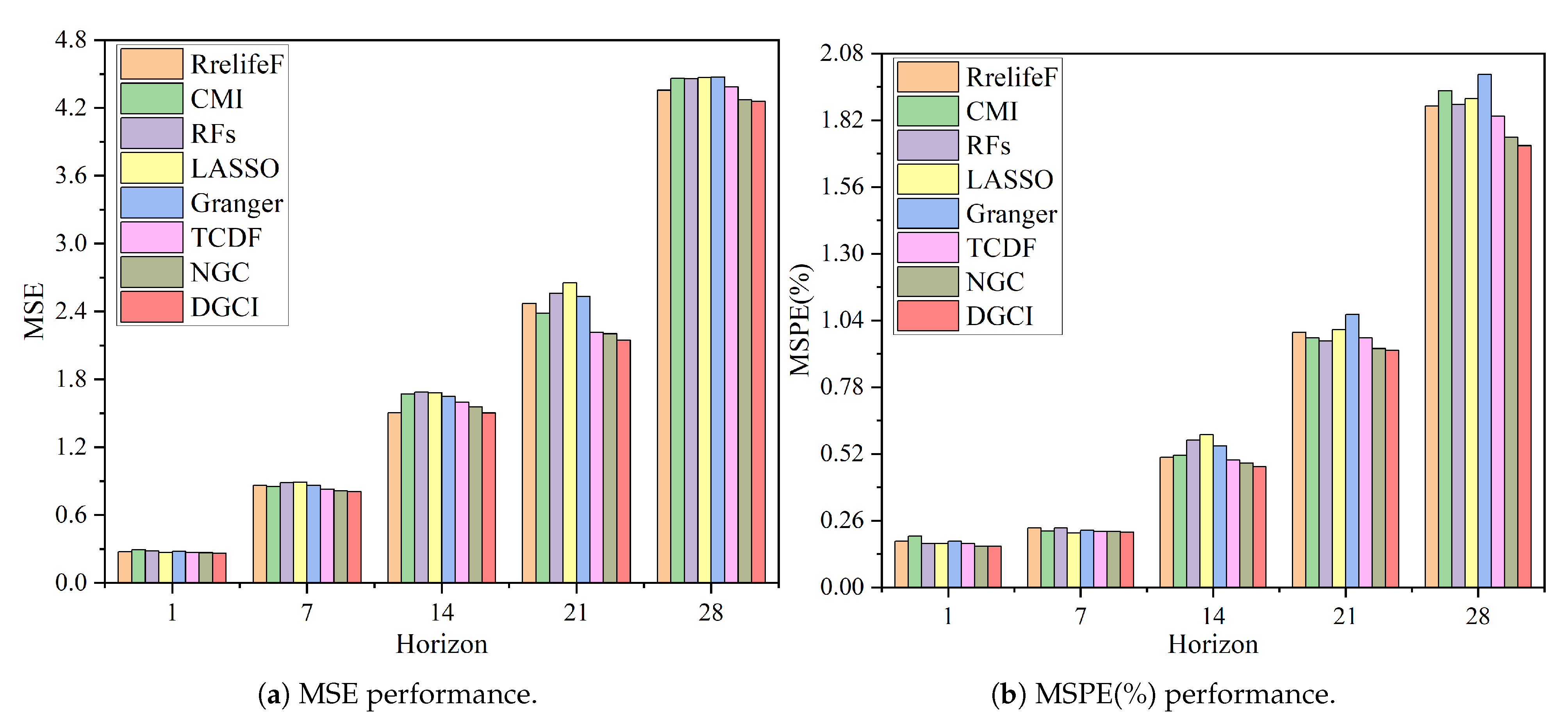
Figure 3 illustrates the performance comparison of all models under varying forecasting horizons, evaluated by MSE and MSPE. Overall, the proposed DGCI model consistently achieves the lowest prediction errors across nearly all horizons, confirming its robustness and adaptability in multi-horizon forecasting. The error growth of DGCI with increasing horizon length is significantly slower than that of the baseline methods, demonstrating its enhanced capacity to capture both short-term and long-term dependencies through dynamic causal interaction learning.

In short-term forecasting (one- and seven-step horizons), DGCI exhibits highly competitive accuracy, performing comparably to or better than other causal discovery models such as NGC and TCDF. The differences among models are relatively minor in this range, as short-term predictions mainly rely on recent temporal information where traditional and deep causal models still retain comparable expressiveness. Nevertheless, DGCI maintains the lowest overall loss, indicating that even in simple temporal regimes, its graph-based causal feature selection contributes to more stable predictions.

As the forecasting horizon extends to medium- and long-term ranges (14-, 21-, and 28-step), the advantages of DGCI become more pronounced. Competing methods show a clear degradation trend due to accumulated temporal uncertainty and weakened feature relevance, whereas DGCI exhibits smoother performance deterioration and retains superior forecasting accuracy. This sustained stability highlights DGCI’s ability to capture persistent causal structures and adaptively refine feature dependencies across time.

Overall, these observations confirm that DGCI not only enhances predictive accuracy but also ensures long-horizon stability through causal inference, demonstrating clear advantages over both conventional feature selection methods and recent deep temporal causality models such as TCDF and NGC.

4.5. Sensitivity Analysis and Ablation Study

4.5.1. Sensitivity Analysis of Feature Size

To assess the stability of DGCI across varying feature scales, this section compares all benchmarks using different feature sizes $F=\{3,5,7,9\}$. The iTransformer predictor, previously shown to perform exceptionally well, is used. The 1-step and 28-step horizons are chosen to represent short- and long-term forecasting, respectively. Table 4 and

Table 5. MSE and MSPE performance under varying feature sizes for 28-step forecasting. The best results are bolded in each column.

Method	F = 3		F = 5		F = 7		F = 9
	MSE	MSPE (%)	MSE	MSPE (%)	MSE	MSPE (%)	MSE	MSPE (%)
RreliefF	4.1644	1.65	4.3564	1.77	4.1153	1.63	4.2051	1.67
CMI	4.4799	1.80	4.4611	1.94	4.1207	1.64	4.2064	1.68
RFs	4.1684	1.66	4.4580	1.81	4.1892	1.69	4.1562	1.65
LASSO	4.2521	1.70	4.4657	1.91	4.2403	1.72	4.1543	1.66
Granger	4.2745	1.71	4.4726	1.98	4.1732	1.65	4.2148	1.69
TCDF	4.1834	1.67	4.3854	1.84	4.0614	1.62	4.1468	1.65
NGC	4.1536	1.62	4.2725	1.75	3.9768	1.60	4.1073	1.65
DGCI	4.1988	1.67	4.2572	1.72	3.9135	1.58	4.0902	1.61

present the MSE results for these horizons, where F represents the number of features. The results demonstrate consistent superiority across both forecasting horizons and feature dimensions.

Table 4. MSE and MSPE (%) loss under varying feature sizes for 1-step forecasting. The best results are bolded in each column.

Method	F = 3		F = 5		F = 7		F = 9
	MSE	MSPE (%)	MSE	MSPE (%)	MSE	MSPE (%)	MSE	MSPE (%)
RreliefF	0.3214	0.20	0.2738	0.18	0.2732	0.17	0.2751	0.18
CMI	0.3660	0.24	0.2949	0.20	0.3155	0.21	0.2967	0.20
RFs	0.3162	0.21	0.2840	0.19	0.2826	0.18	0.2717	0.17
LASSO	0.3302	0.22	0.2703	0.18	0.2750	0.18	0.2722	0.17
Granger	0.3445	0.23	0.2783	0.19	0.2847	0.19	0.2736	0.18
TCDF	0.3284	0.19	0.2699	0.17	0.2722	0.17	0.2681	0.16
NGC	0.3124	0.18	0.2657	0.16	0.2693	0.16	0.2657	0.15
DGCI	0.3323	0.22	0.2623	0.15	0.2710	0.16	0.2631	0.16

Table 4. MSE and MSPE (%) loss under varying feature sizes for 1-step forecasting. The best results are bolded in each column.

Method	F = 3		F = 5		F = 7		F = 9
	MSE	MSPE (%)	MSE	MSPE (%)	MSE	MSPE (%)	MSE	MSPE (%)
RreliefF	0.3214	0.20	0.2738	0.18	0.2732	0.17	0.2751	0.18
CMI	0.3660	0.24	0.2949	0.20	0.3155	0.21	0.2967	0.20
RFs	0.3162	0.21	0.2840	0.19	0.2826	0.18	0.2717	0.17
LASSO	0.3302	0.22	0.2703	0.18	0.2750	0.18	0.2722	0.17
Granger	0.3445	0.23	0.2783	0.19	0.2847	0.19	0.2736	0.18
TCDF	0.3284	0.19	0.2699	0.17	0.2722	0.17	0.2681	0.16
NGC	0.3124	0.18	0.2657	0.16	0.2693	0.16	0.2657	0.15
DGCI	0.3323	0.22	0.2623	0.15	0.2710	0.16	0.2631	0.16

In short-term forecasting (one-step), the proposed DGCI model consistently achieves superior predictive accuracy across all feature sizes, as reported in Table 4. The model attains its best performance at $F=5$, reaching an MSE of 0.2623 and an MSPE of 0.15%, which outperforms all other benchmark methods. Notably, DGCI continues to deliver stable and competitive performance as the feature dimension increases, maintaining an MSE of 0.2631 and an MSPE of 0.16% at $F=9$. With the introduction of the recent deep causal models, TCDF and NGC, the comparative landscape becomes more competitive. Among them, NGC emerges as the next-best causal baseline, achieving an MSE of 0.2657 and MSPE of 0.16% at $F=5$, closely approaching DGCI’s performance. This narrow margin highlights DGCI’s robustness in enhancing predictive precision beyond established causal discovery methods. Meanwhile, DGCI demonstrates moderate yet stable performance improvements compared to classical approaches such as Granger causality and LASSO. Empirical evidence reveals a non-monotonic relationship between feature quantity and predictive efficacy in short-term forecasting.

In long-term forecasting (28-step), the MSE and MSPE losses of all methods are generally higher than in short-term forecasting due to the increased complexity of long-horizon dependencies, as shown in Table 5. Among the compared models, DGCI consistently demonstrates the lowest MSE and MSPE values at $F=\{5,7,9\}$, reaffirming its stability in feature selection across varying prediction horizons and its superiority in handling long-term dependencies. Notably, at $F=7$, DGCI achieves the best performance (MSE = 3.9135 and MSPE = 1.58%), indicating its enhanced ability to identify critical features and capture complex spatiotemporal interactions. Compared with TCDF and NGC, both of which explicitly model temporal causality, DGCI yields lower errors across all feature sizes. While NGC exhibits competitive results at smaller feature sets (e.g., achieving MSE = 4.1536 and MSPE = 1.62% at $F=3$), its performance improvement saturates as the feature dimension increases. In contrast, DGCI continues to achieve progressive gains, maintaining sustained leadership at $F=9$ (MSE = 4.0902 and MSPE = 1.61%).

From both tables, DGCI shows excellent performance in both short- and long-term predictions, with its MSE and MSPE values remaining at almost the lowest level for different feature numbers, indicating its high stability. In contrast, other baseline methods exhibit greater performance fluctuations across different feature counts and generally have higher MSE and MSPE values than DGCI. This implies that these methods are relatively less stable and effective in feature selection, possibly due to their limitations in handling complex feature relationships and uncertainties arising from different prediction time spans.

4.5.2. Sensitivity Analysis of Hyperparameters

In the proposed framework, the CFI score is defined as a weighted combination of the feature reconstruction loss and the causality loss. Since the relative magnitudes of these two terms may vary across datasets, a sensitivity analysis on the hyperparameters ${\lambda }_1$ and ${\lambda }_2$ is necessary to ensure the robustness of the metric. To reduce the complexity of hyperparameter search, we first fixed ${\lambda }_1=1$ and varied ${\lambda }_2$ in the range of $[10,20]$. This setup allows us to examine how different relative weightings between $Los{s}_{rec}$ and $Los{s}_{cau}$ affect the model’s performance. The predictive performance of different ${\lambda }_2$ is presented in Figure 4.

The performance shows a non-monotonic pattern, suggesting a trade-off between representation fidelity and predictive causality. Among the tested values, ${\lambda }_2=15$ achieves the best performance, with MSE = 0.2623 and MSPE = 0.15%. This confirms that balancing the two objectives at the ratio ${\lambda }_1$:${\lambda }_2$ = 1:15 yields the most stable and accurate results. The results indicate that smaller or larger values of ${\lambda }_2$ degrade performance. When ${\lambda }_2$ is too small, the causality contribution is underweighted, leading to incomplete characterization of feature importance. Conversely, overly large values of ${\lambda }_2$ cause the causality term to dominate excessively, which results in instability and degraded accuracy.

Although the optimal ratio is identified as ${\lambda }_1$:${\lambda }_2$ = 1:15, the absolute magnitudes of $\lambda$ also influence the scale of the final CFI values. To avoid inflated CFI scores and improve interpretability, we performed a proportional rescaling, reducing both hyperparameters while preserving their ratio. The final choice ${\lambda }_1=0.1$ and ${\lambda }_2=1.5$ maintains the optimal balance but ensures that the resulting CFI values remain within a more interpretable numerical range. This adjustment does not affect relative rankings of feature importance but improves consistency and comparability across datasets.

4.5.3. Ablation Study

To further evaluate the contribution of individual components within the proposed DGCI model, we conducted a set of ablation experiments. Specifically, three model variants are compared as follows:

• DGCI-Direct: The FRM is completely removed. The raw input sequence $X_t$ is directly fed into the Granger Causality Module without any dimensionality reduction. This variant serves as a baseline to evaluate the necessity of feature reconstruction.
• DGCI-VAE: The FRM was simplified to contain only a VAE, without Transformer-based temporal attention. This configuration allows us to isolate the effectiveness of incorporating Transformer structures within the FRM.
• DGCI-Full: The complete model proposed in this work, integrating both VAE and Transformer within the FRM. This version fully leverages the strengths of compact representation learning and global temporal dependency modeling.

The results of the ablation study are shown in

Table 6. Results of ablation study on different model variants. The symbols ✓ and × denote whether the corresponding module is included or not included, respectively. The best results are bolded in each column.

Method	FRM	VAE	MSE	MSPE (%)
DGCI-Direct	×	×	0.3264	0.1835
DGCI-VAE	×	✓	0.2817	0.1634
DGCI-Full	✓	✓	0.2623	0.1500

, which reveals three key observations: First, DGCI-Direct performs the worst, confirming that feeding raw high-dimensional inputs directly into the causality module leads to poor generalization. This highlights the necessity of a reconstruction-based representation learning step. Second, DGCI-VAE achieves clear improvements over DGCI-Direct, indicating that even a pure VAE-based dimensionality reduction contributes to filtering out noise and extracting more informative latent features. Third, DGCI-Full achieves the best performance, with the lowest MSE and MSPE. The inclusion of Transformer mechanisms within FRM further enhances the representation by capturing long-range temporal dependencies and cross-variable interactions, which a vanilla VAE cannot fully exploit.

This ablation analysis demonstrates that both the VAE-based dimensionality reduction and the Transformer-enhanced representation learning are indispensable for achieving optimal performance. The stepwise improvement confirms that the proposed FRM design is effective and that its synergy with the causality module significantly boosts the robustness and accuracy of causal feature inference.

4.6. Key Feature Interpretation Analysis

The proposed DGCI model calculates the CFI values for 16 features, ranking them to identify core features.

Table 7. Quantitative ranking of CFI via DGCI model.

Loss Type	Variables
	$X_{\mathit{pork}}$	$X_{\mathit{piglet}}$	$X_{\mathit{slau}}$	$X_{\mathit{feed}}$	$X_{\mathit{ratio}}$	$X_{\mathit{fatten}}$	$X_{\mathit{cpi}}$	$X_{\mathit{corn}}$
$Los{s}_{rec}$	5.2622	6.1225	6.7769	8.2986	5.6523	3.2108	3.4542	2.4940
$Los{s}_{cau}$	0.6636	0.5552	0.4993	0.3801	0.3466	0.4568	0.3580	0.3754
$CFI$	1.5216	1.4451	1.4266	1.4000	1.0851	1.0063	0.8824	0.8125
Loss type	Variables
	$X_{pfr}$	$X_{hog}$	$X_{ppi}$	$X_{bean}$	$X_{ipq}$	$X_{sow}$	$X_{supply}$	$X_{ipa}$
$Los{s}_{rec}$	4.2992	6.9089	5.1957	1.4098	1.3947	6.0056	4.6971	1.5647
$Los{s}_{cau}$	0.2173	0.0354	−0.0389	0.1962	0.0601	−0.2776	−0.2756	−0.2612
$CFI$	0.7559	0.7440	0.4612	0.4353	0.2296	0.1842	0.0563	−0.2353

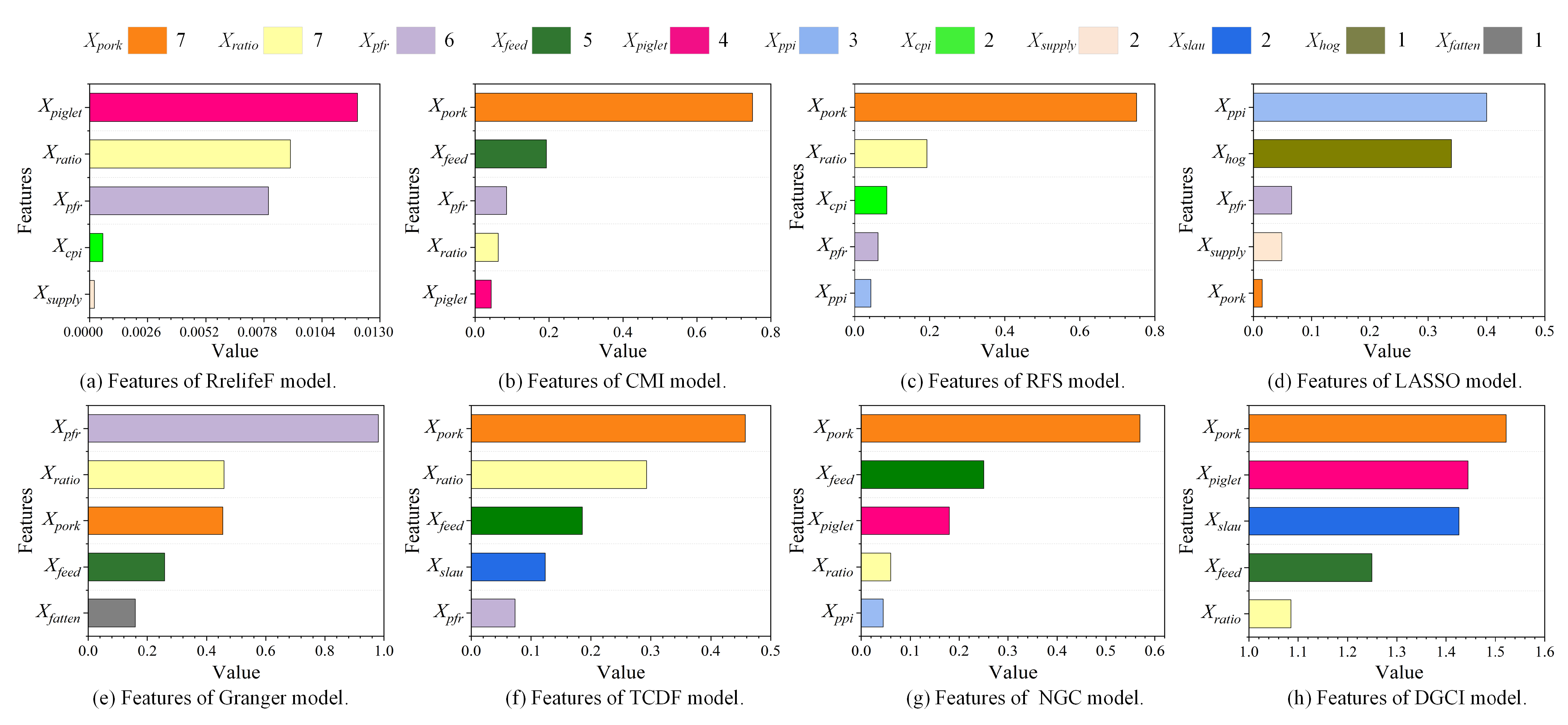
presents the CFI values to validate each feature’s information complexity and causal effects. Figure 5 visually compares the top five features selected by the proposed DGCI model and the other five baseline models, intuitively revealing the feature selection reliability of DGCI model.

In Table 7, the DGCI computes CFI values, along with reconstruction loss ($Los{s}_{rec}$) and Granger loss ($Los{s}_{cau}$), which are presented for all 16 features. CFI is a weighted sum of $Los{s}_{rec}$ and $Los{s}_{cau}$, with weights ${\lambda }_1=0.1$ and ${\lambda }_2=1.5$ from prior sensitivity analysis. High $Los{s}_{rec}$ features (e.g., feed price $X_{feed}$ of 8.2986, hog inventory $X_{hog}$ of 6.9089) show significant information loss in compressed representation, implying complex nonlinear patterns between multivariate. High $Los{s}_{cau}$ features (e.g., pork price $X_{pork}$ of 0.6636 and piglet price $X_{piglet}$ of 0.5552) have a strong causal impact on hog price forecasting, working through supply-demand, cost transmission, and market linkages. The CFI metric synthetically integrates these informational and causal dimensions, with the highest values identifying pork price ($X_{pork}$), piglet price ($X_{piglet}$), slaughter volume ($X_{slau}$), feed price ($X_{feed}$), and national pig-feed ratio ($X_{ratio}$) as paramount features. $X_{pork}$ functions as a terminal price signal directly driving hog pricing, $X_{piglet}$ serves as a leading cost indicator presaging price trends, $X_{slau}$ dictates immediate supply-demand balance, $X_{feed}$ underpins cost structure fundamentals, while $X_{ratio}$ reflects breeder profitability thresholds that govern production cycles.

Figure 5 illustrates the top five features selected by all models, providing an overall view of the feature importance distribution. As shown, several features are consistently selected across different models, indicating their strong relevance to hog price dynamics. Specifically, $X_{pork}$ (pork price) and $X_{ratio}$(national pig-feed ratio) are the most frequently chosen features, each identified by seven models. Other highly ranked features include $X_{pfr}$ (pork-feed ratio, selected by six models), $X_{feed}$ (feed price, selected by five models), and $X_{piglet}$ (piglet price, selected by four models). Notably, the DGCI model identifies $X_{pork}$, $X_{piglet}$, $X_{slau}$ (hog slaughter volume), $X_{feed}$, and $X_{ratio}$ as its top five features (Figure 5h). These features largely overlap with those frequently selected by other models, suggesting that the DGCI framework captures both domain-consistent and model-robust predictors. This consistency further validates the effectiveness and interpretability of the proposed feature selection mechanism.

The DGCI model identifies pork price as the most critical determinant, with the highest CFI value (1.5216), underscoring its central role as a causal signal in price transmission. Although hog price and pork price are highly correlated, they capture different positions in the supply chain. Hog price reflects the upstream production market, while pork price represents the terminal consumer market. Pork price directly responds to shifts in consumer demand and retail dynamics, which in turn feed back to influence slaughter decisions and production adjustments in the hog sector. The fluctuations in pork price not only guide consumer purchasing behavior but also shape the production side by affecting slaughter plans and farming scale. The pork price can serve as a key monitoring indicator for government interventions, including the release of pork reserves and the implementation of price stabilization measures. Fluctuations in pork prices convey essential signals throughout the distribution and retail chains, facilitating coordinated adjustments across the entire industry value chain.

Piglet cost is a critical input in the farming process, directly affecting production costs and profit margins. When piglet costs rise, farming expenses increase, potentially leading to reduced hog supply and higher hog prices. The relatively high CFI value highlights the significant influence of piglet cost on the supply side and its importance in shaping market price formation. Piglet costs directly determine the input-output relationship in the breeding process and are closely related to feed utilization efficiency and farming profitability, which affects the sustainable use of agricultural resources. The piglet cost can indirectly influence supply elasticity through targeted policy instruments such as production subsidies for hog farming, feed price adjustments, and financial support for breeding expenditures.

Slaughter volume reflects the actual scale of market supply and serves as a key indicator of supply-demand balance in the hog market. Changes in slaughter volume are driven by factors such as farming output, market demand, and policy interventions. A reduction in slaughter volume may lead to insufficient supply and higher hog prices, while an increase in slaughter volume could suppress prices. Its CFI value underscores the sensitivity and importance of slaughter volume in hog price fluctuations. Slaughter volume is crucial for preventing overproduction or supply shortages through rational regulation, thereby maintaining market sustainability. The slaughter volume functions as an important metric for evaluating supply–demand imbalances and guiding the timing of slaughtering operations and market releases.

These three factors collectively form the core driving mechanism of hog price dynamics, encompassing demand-side (pork price), cost-side (piglet cost), and supply-side (slaughter volume) influences. From a practical perspective, uncovering these determinants provides actionable implications for both policymakers and farmers. For the government, real-time monitoring of pork prices, piglet costs, and slaughter volume can serve as early warning indicators for market volatility. By tracking these factors, authorities can better time the release of pork reserves, adjust subsidies, and guide breeding and slaughtering cycles, thereby smoothing sharp price fluctuations and protecting consumer welfare. For pig farmers, the identified features offer a scientific basis for production and investment decisions. Stabilizing piglet procurement costs and optimizing slaughter timing according to market signals can reduce operational risks and improve profitability. In this way, the DGCI model not only advances the understanding of causal price drivers but also supports the design of more effective policy tools and adaptive farming strategies to enhance the resilience and sustainability of the swine industry.

While the DGCI model identifies these factors as the most influential determinants of market dynamics, it is noteworthy that several external factors also exert significant yet more indirect effects. The comparatively low CFI values of these external variables indicate that, during the observation period, their causal influences on live pig prices were largely mediated or overshadowed by more immediate production- and cost-related mechanisms. For instance, while the volume and value of pork imports can theoretically alter the domestic supply-demand equilibrium, China’s pork import volume constitutes only a minor fraction of total national consumption under normal conditions, thereby exerting a limited effect on domestic price formation. Similarly, domestic pork consumption has remained relatively stable in relation to production levels, and the country’s modest macroeconomic fluctuations have had negligible influence on household pork demand. Consequently, the external economic environment, as proxied by the CPI, demonstrates only a marginal contribution to short-term pork price volatility. Moreover, China’s industrial policies are primarily designed to regulate the prospective production capacity of the pig industry, ensuring output stability over future months. As such, their regulatory effects tend to exhibit a substantial temporal lag—often six months or longer—rendering their short-run impact on pork prices considerably weaker than that of more immediate market indicators.

5. Conclusions

China’s swine sector plays a pivotal role in maintaining national economic equilibrium and influencing global agricultural dynamics. Nevertheless, intricate multifactorial elements contribute to volatility within hog trading markets. This study proposes the Deep Granger Causality Inference (DGCI) framework to uncover nonlinear causal relationships underlying China’s swine market dynamics. The DGCI framework innovatively combines deep learning with causal inference, achieving both interpretability and predictive performance while effectively identifying key drivers of hog price fluctuations.

Empirical assessment employs a comprehensive national swine dataset encompassing 16 variables across supply-side, cost-related, and external factors. DGCI undergoes rigorous evaluation against established feature selection methodologies using five prediction models and various horizons (1–28 days). Performance enhancement metrics demonstrate considerable gains, with DGCI decreasing MSE by 17.59% to 39.22% and MSPE by 32.35% to 54.90% relative to comparison methods. The model identifies pork price, piglet cost, and slaughter volume as critical causal determinants of hog price, with CFI values of 1.5216, 1.4451, and 1.4266, respectively. By revealing dynamic causal relationships across supply, demand, and cost dimensions, DGCI provides actionable insights for production planning and market stabilization interventions. The interdisciplinary integration of machine learning with agricultural economics demonstrates how computational methodologies can enhance traditional livestock research paradigms, expanding the analytical framework for swine industry studies.

Importantly, although the empirical analysis of this study is confined to the Chinese hog market, the DGCI framework itself is not limited to this context. Its ability to capture nonlinear, multivariate Granger-causal relationships makes it broadly applicable to other livestock markets, where complex temporal dependencies and causal dynamics are prevalent. This generalizability underscores the potential of DGCI to serve as a versatile analytical tool, enabling researchers and practitioners across disciplines to investigate causal drivers and enhance forecasting under diverse market conditions. Future research should explore DGCI’s adaptability to broader commodity markets and integrate dynamic risk assessment capabilities to enhance resilience under volatile conditions. Additionally, incorporating biological and environmental variables (feed quality, disease outbreaks, climate conditions) could strengthen the model’s explanatory power, while developing real-time monitoring systems would support policymakers in market stabilization efforts.