Unsupervised Convolutional Transformer Autoencoder for Robust Health Indicator Construction and RUL Prediction in Rotating Machinery

Abstract

Prognostics for rotating machinery, particularly bearings, encounter significant challenges in constructing reliable health indicators (HIs) that accurately reflect degradation trajectories, thereby enabling precise remaining useful life (RUL) predictions. This article proposes a novel integrated approach for predicting the RUL of bearings without manual feature engineering. Specifically, a sequential autoencoder integrating a convolutional neural network (CNN) and vision Transformer (Vi-T) is employed to capture the local spatial patterns and global temporal correlations of time-domain vibration signals. The Wasserstein distance is introduced to quantify the divergence between healthy and degraded signal embeddings, resulting in a robust HI metric. Subsequently, the derived HI is fed into a CNN-bidirectional long short-term memory-regressor with Monte Carlo dropout to provide RUL predictions and Bayesian uncertainty estimates. Experimental results from the Xi’an Jiao-Tong University bearing dataset demonstrate that the proposed method surpasses conventional techniques in HI construction and RUL prediction accuracy, demonstrating its efficacy for complex industrial systems with minimal data preprocessing.

1. Introduction

In parallel with the burgeoning advancements in industrial Internet of Things, artificial intelligence algorithms, and computational capabilities, DL-based data-driven methodologies have emerged as predominant paradigms in PHM for rotating machinery [1,2,3]. Bearings, as critical components in sectors such as power generation, aerospace, and manufacturing, directly affect system reliability and performance, so accurate RUL estimation is essential for facilitating predictive maintenance, reducing unplanned downtimes, and ultimately extending the operational lifespan of machinery [4,5,6,7,8]. RUL prediction approaches are dichotomized into physics-based models [9,10], which demand intricate mechanical insights and precise simulations, and data-driven models [11,12,13], which harness operational data to discern degradation patterns, offering adaptability to multifaceted systems sans profound physical domain knowledge. Consequently, data-driven techniques are increasingly favored for handling the large and high-dimensional datasets common in modern predictive maintenance.

Constructing efficacious data-driven RUL models entails four pivotal stages: sensor data acquisition and preprocessing (e.g., denoising, normalization, dimensionality reduction); degradation feature extraction and health indicator (HI) formulation, which combines signal processing with domain expertise; FPT detection; and RUL regression using machine learning [14]. The HI construction is critical because it determines how faithfully degradation is represented and thus influences prediction accuracy. In this regard, Dong et al. [15] applied principal component analysis to combine the features, which were then input into a weighted complex support vector machine model to predict the RUL of bearings. Similarly, Guo et al. [16] introduced a degradation indicator for predicting the RUL of bearings, utilizing EMD. Zhang et al. [17] proposed a method that combines multi-scale entropy features as a health indicator for accurate RUL prediction of rolling bearings. Zhao et al. [18] employed a method for RUL prediction of rolling bearings that focuses on modeling degraded features using the derivative method of the fitting curve for maximum power spectral density. Long et al. [19] introduced a method for RUL prediction of rolling bearings that emphasizes the creation of HI based on EMD, refined composite multi-scale attention entropy, and dispersion entropy. These studies primarily relied on signal processing techniques to extract features from raw signals in order to develop degradation indicators. These methods are advantageous due to their clear physical interpretation and ease of validation. However, signal processing-based feature extraction has its limitations. The techniques often depend on expert knowledge and experience, may lack generalizability across equipment types, and can miss implicit nonlinear features present in complex data.

Conversely, DL paradigms automate HI extraction from raw vibrations. For instance, [20] was a pioneer in applying recurrent neural networks to autonomously extract HIs from selected features, creating an early data-driven framework to characterize the deterioration of rolling bearings. Similarly, Ref. [21] utilized a hybrid model combining CNN and bidirectional gated recurrent units to derive HIs from raw vibrational signals for roller bearings. Li et al. [22] used a multi-channel fusion hierarchical vision Transformer with wavelet packet decomposition representations to model degraded features for RUL prediction. Guo et al. [23] proposed a hybrid approach that initially constructs a nonlinear HI using complete ensemble empirical mode decomposition with adaptive noise and kernel principal component analysis. They then extracted multi-domain features from vibration signals and applied a dual-channel Transformer network with convolutional attention modules to generate HIs for other bearings. Ping et al. [24] proposed a multi-scale efficient channel attention convolutional neural network and bidirectional gated recurrent unit model for RUL prediction of rolling bearings, extracting multi-scale temporal features from Gram’s angle difference field images. Notwithstanding advancements, these predominantly supervised techniques necessitate abundant labeled data, impeding applicability in prevalent, unlabeled real-world industrial scenarios.

To facilitate data-driven automatic construction of HIs, this study investigates unsupervised learning paradigms. Autoencoders provide a viable framework, enabling label-agnostic HI development through feature extraction and degradation trend modeling. Guo et al. [25] proposed an unsupervised HI construction method using a multi-scale convolutional autoencoder optimized by a genetic algorithm, effectively identifying machine degradation through feature learning and data similarity. Ma et al. [26] developed a self-attention convolutional autoencoder, demonstrating enhanced trendability and scale similarity on bearing and milling cutter datasets. Xu et al. [27] proposed an enhanced stacked autoencoder with an exponential weighted moving average for health indicator construction using unlabeled vibration signals, improving noise reduction and eliminating the need for manual feature selection. De et al. [28] developed an LSTM autoencoder with attention for health indicator construction in aircraft systems. Xu et al. [29] developed a multi-scale-multi-head attention mechanism with an automatic encoder–decoder model, extracted multi-scale features from raw vibration signals, and measured the Wasserstein distance between healthy and unhealthy features, which demonstrated superiority over other similarity-based methods and provided a more reliable HI. Qu et al. [30] proposed an unsupervised method for bearing health indicator construction using multi-scale convolution and long short-term memory combined with an autoencoder for feature extraction and support vector regression to build health indicators, improving degradation trend detection. Wang et al. [31] developed a denoising Transformer autoencoder for tool condition monitoring, enhancing feature extraction and resistance to noise.

Although autoencoders are extensively employed in existing studies for unsupervised feature learning, they exhibit shortcomings in processing time-series signals, particularly in capturing the temporal dependencies of encoded features. Additionally, conventional HI construction techniques frequently necessitate manual selection and design of dominant features, rendering them inefficient and error-prone, especially with high-dimensional or nonlinear datasets. This reliance on manual feature engineering can lead to inaccurate similarity measurements and diminished HI fidelity. To address these challenges, this paper proposes an HCVT-WD for bearing HI construction and RUL prediction. The proposed method encompasses four key stages: (1) an unsupervised HCVT-WD autoencoder framework is developed to extract features from FFT-transformed raw vibration signals without manual feature engineering or labeling; (2) CNN and Vi-T are integrated to captures local spatial patterns and global temporal correlations; (3) Wasserstein distance is used to quantify divergences between healthy for robust HI formulation; and (4) an HI driven RUL prediction pipeline provides accurate forecasts with uncertainty quantification.

The structure of the paper is as follows: Section 2 focuses on the proposed framework, specifically highlighting the development of HIs using the proposed HCVT-WD model. Section 3 details the experimental setup, results, and analysis. Section 4 provides a summary of the key results and proposes possible directions for future studies.

2. Proposed Framework

The overall workflow of the proposed method is illustrated in Figure 1, with a detailed clarification of the HI construction process provided in Algorithm 1. In the initial phase, the HCVT-WD model is trained using a subset of the dataset ${\left\{{\mathrm{x}}_{\mathrm{i}}^{\mathrm{t}\mathrm{r}\mathrm{a}\mathrm{i}\mathrm{n}}\right\}}_{\mathrm{i}=1}^{{\mathrm{N}}_{\mathrm{t}\mathrm{r}\mathrm{a}\mathrm{i}\mathrm{n}}}$ composed of non-overlapping windows extracted from vibration signals recorded during healthy operation. ${\mathrm{N}}_{\mathrm{t}\mathrm{r}\mathrm{a}\mathrm{i}\mathrm{n}}$ refers to the number of time instances, with each instance corresponding to a specific time window from the healthy state data. The training process minimizes the reconstruction error of the network. Once trained, the encoded features from the HCVT-WD are extracted. In the next phase, the model is implemented on the whole dataset ${\left\{{\mathrm{x}}_{\mathrm{i}}^{\mathrm{t}\mathrm{e}\mathrm{s}\mathrm{t}}\right\}}_{\mathrm{i}=1}^{{\mathrm{N}}_{\mathrm{t}\mathrm{e}\mathrm{s}\mathrm{t}}}$, which consists of both healthy and unhealthy state data samples, similarly done for the training dataset. The WD between the combined encoded features of the healthy state and the encoded features of all other states is computed and used as the HI. Finally, the HI is modeled using a CNN-BiLSTM network with MC simulations to predict the RUL and quantify uncertainty.

Algorithm 1 Train the HCVT-WD model and construct HI

Input: Frequency domain raw vibrational signals (healthy and unhealthy states): ${\mathrm{x}}_{\mathrm{i}}^{\mathrm{r}\mathrm{a}\mathrm{w}}\in {ℝ}^{\mathrm{L}\times \mathrm{C}}$ and initial parameters $\mathrm{\theta }$. Build and Initialize: HCVT-WD model. Consider training data ${\left\{{\mathrm{x}}_{\mathrm{i}}^{\mathrm{t}\mathrm{r}\mathrm{a}\mathrm{i}\mathrm{n}}\right\}}_{\mathrm{i}=1}^{{\mathrm{N}}_{\mathrm{t}\mathrm{r}\mathrm{a}\mathrm{i}\mathrm{n}}}$ as healthy data and ${\left\{{\mathrm{x}}_{\mathrm{i}}^{\mathrm{t}\mathrm{e}\mathrm{s}\mathrm{t}}\right\}}_{\mathrm{i}=1}^{{\mathrm{N}}_{\mathrm{t}\mathrm{e}\mathrm{s}\mathrm{t}}}$ as whole data. While $\mathrm{i}\le \mathrm{E}\mathrm{p}\mathrm{o}\mathrm{c}\mathrm{h}\mathrm{s}$ do    Decoded output ${\widehat{\mathrm{x}}}_{\mathrm{i}}^{\mathrm{t}\mathrm{r}\mathrm{a}\mathrm{i}\mathrm{n}}$ from model.    Minimize loss between ${\mathrm{x}}_{\mathrm{i}}^{\mathrm{t}\mathrm{r}\mathrm{a}\mathrm{i}\mathrm{n}}$ and ${\widehat{\mathrm{x}}}_{\mathrm{i}}^{\mathrm{t}\mathrm{r}\mathrm{a}\mathrm{i}\mathrm{n}}$.    $\mathrm{\theta }\leftarrow$ Update parameters of the model. End for Obtain encoded features ${\mathrm{Z}}_{\mathrm{t}\mathrm{r}\mathrm{a}\mathrm{i}\mathrm{n}}$ and ${\mathrm{Z}}_{\mathrm{t}\mathrm{e}\mathrm{s}\mathrm{t}}$ along with trained HCVT-WD model parameters ${\mathrm{\theta }}^{*}$. Calculate the Wassertian distance between encoded ${\mathrm{Z}}_{\mathrm{t}\mathrm{r}\mathrm{a}\mathrm{i}\mathrm{n}}$ and ${\mathrm{Z}}_{\mathrm{t}\mathrm{e}\mathrm{s}\mathrm{t}}$ as HI. $\mathrm{H}{\mathrm{I}}_{\mathrm{j}}=\mathrm{W}\mathrm{D}\left({\mathrm{Z}}_{\mathrm{t}\mathrm{e}\mathrm{s}\mathrm{t},\mathrm{j}},{\mathrm{Z}}_{\mathrm{t}\mathrm{r}\mathrm{a}\mathrm{i}\mathrm{n}}\right)={\displaystyle \frac{1}{{\mathrm{N}}_{\mathrm{t}\mathrm{r}\mathrm{a}\mathrm{i}\mathrm{n}}}}{\displaystyle \sum _{\mathrm{i}=1}^{{\mathrm{N}}_{\mathrm{t}\mathrm{r}\mathrm{a}\mathrm{i}\mathrm{n}}}\parallel {\mathrm{z}}_{\mathrm{j}}-}{\mathrm{z}}_{\mathrm{i}}{\parallel }_1$ Detect the FPT using $\mathrm{\mu }\pm 3\mathrm{\sigma }$ Output: $\mathrm{H}{\mathrm{I}}_{\mathrm{j}}$, FPT

2.1. HCVT Autoencoder Model

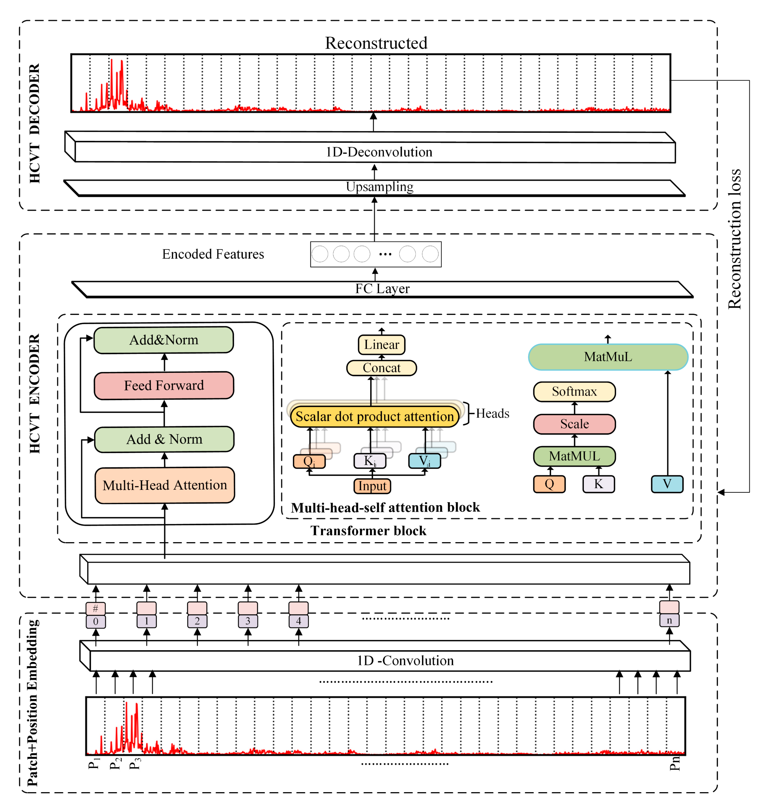
In this section, we employ a hybrid model consisting of 1D-CNN and Vi-T as the encoder. The encoder extracts deep features from the inputs using the combined strengths of CNN and Vi-T architectures, and these encoded features are then upsampled to the original image dimensions using a CNN-based decoder.

2.1.1. 1D-CNN Patch and Position Embedding

To process time series data effectively, the signal is first split into smaller segments. Patch embedding serves this purpose before applying the Vi-T to time series data, as it enables the Transformer model to process both one-dimensional and multi-dimensional time series data effectively.

The raw vibrational signals are initially segmented into non-overlapping segments. Denote each segment by ${{\mathrm{X}}_{\mathrm{i}}}^{\mathrm{r}\mathrm{a}\mathrm{w}}\in {ℝ}^{\mathrm{L}\times \mathrm{C}}$, where $\mathrm{L}$ and $\mathrm{C}$ are the length of the segments and the dimension of the input signals. Each segment is further partitioned into fixed-size patches. Each patch is represented as ${\mathrm{x}}_{\mathrm{i}}^{\mathrm{p}}\in {ℝ}^{{\mathrm{L}}_{\mathrm{p}}\times \mathrm{C}}$, where ${\mathrm{L}}_{\mathrm{p}}$ is the length of each patch. It can be deduced to $\mathrm{L}={\mathrm{L}}_{\mathrm{p}}\times \mathrm{m}$, where $\mathrm{m}$ is the number of patches. One-dimensional convolution operation is then applied to each patch as shown in Equation (1). The size of the convolution kernel is identical to that of patch $\mathrm{p}$, and the stride is ${\mathrm{L}}_{\mathrm{p}}$, to preserve the temporal dynamics in the raw signals.

$${\mathrm{d}}_{\mathrm{p}}^{\mathrm{k}}={\displaystyle {\sum }_{\mathrm{i}=0}^{{\mathrm{L}}_{\mathrm{p}}-1}{\displaystyle {\sum }_{\mathrm{j}=0}^{\mathrm{C}-1}\mathrm{p}(\mathrm{i},\mathrm{j})}\times {\mathrm{w}}^{\mathrm{k}}(\mathrm{i},\mathrm{j})+{\mathrm{b}}^{\mathrm{k}},1\le \mathrm{k}\le \mathrm{n}},$$

(1)

where ${\mathrm{w}}^{\mathrm{k}}$ and ${\mathrm{b}}^{\mathrm{k}}$ represent the weight and bias of the k-th convolutional kernel, respectively. The variable denotes the number of convolutional kernels, as well as the dimension of the time-series patch embedding. The term ${\mathrm{d}}_{\mathrm{p}}$ corresponds to the embedding outcome of the patch. The embedding results for the entire set of patches in each sample ${\mathrm{X}}^{\mathrm{r}\mathrm{a}\mathrm{w}}$ are presented in Equation (2).

$${\mathrm{d}}_{\mathrm{p}}=\left[{\mathrm{d}}_{\mathrm{p}}^1,{\mathrm{d}}_{\mathrm{p}}^2,\dots ,{\mathrm{d}}_{\mathrm{p}}^{\mathrm{n}}\right]$$

(2)

Since Vi-T does not inherently recognize the order of patches, positional encoding is incorporated into the patch embeddings to preserve spatial information. For position encoding, each embedded patch is encoded as follows:

$${\mathrm{d}}_{\mathrm{i}}^{\mathrm{P}\mathrm{e}\mathrm{n}\mathrm{c}\mathrm{o}\mathrm{d}\mathrm{e}\mathrm{d}}={\mathrm{d}}_{\mathrm{i}}^{\mathrm{n}}+{\mathrm{d}}_{\mathrm{i}}^{\mathrm{P}\mathrm{o}\mathrm{s}}$$

(3)

where the positions ${\mathrm{d}}_{\mathrm{i}}^{\mathrm{P}\mathrm{o}\mathrm{s}}$ for the i-th patch are defined as follows:

$$\begin{array}{l}{\mathrm{p}}_{\mathrm{i}}^{2\mathrm{k}}=\mathrm{s}\mathrm{i}\mathrm{n}\left(\mathrm{i}/{10000}^{2\mathrm{k}/\mathrm{d}}\right)\\ {\mathrm{p}}_{\mathrm{i}}^{2\mathrm{k}+1}=\cos \left(\mathrm{i}/{10000}^{2\mathrm{k}/\mathrm{d}}\right)\end{array}$$

(4)

where ${\mathrm{p}}_{\mathrm{i}}^{2\mathrm{k}}$ and ${\mathrm{p}}_{\mathrm{i}}^{2\mathrm{k}+1}$ represent the positional encodings for the i-th position within the sequence, and $\mathrm{d}$ is the dimensionality of the feature vectors.

2.1.2. Vision Transformer Encoder

The patch embeddings, augmented with positional encodings, are subsequently processed through an MHSA module. This module is built upon the scaled dot-product attention mechanism, which facilitates interactions between all positions in the sequence. The MHSA architecture extends this principle by employing multiple attention heads in parallel. Each head has independent parameters, and learn distinct attention patterns and captures a diverse set of semantic relationships within the data. A schematic of the MHSA mechanism is illustrated in Figure 2.

The definition of the i-th attention function is defined as follows:

$$\mathrm{h}\mathrm{e}\mathrm{a}{\mathrm{d}}_{\mathrm{i}}=\mathrm{A}\mathrm{t}\mathrm{t}\mathrm{e}\mathrm{n}\mathrm{t}\mathrm{i}\mathrm{o}\mathrm{n}\left(\mathrm{Q}{\mathrm{W}}_{\mathrm{Q}}^{\mathrm{i}},\mathrm{K}{\mathrm{W}}_{\mathrm{K}}^{\mathrm{i}},\mathrm{V}{\mathrm{W}}_{\mathrm{V}}^{\mathrm{i}}\right)$$

(5)

where ${\mathrm{W}}_{\mathrm{Q}}^{\mathrm{i}}$, ${\mathrm{W}}_{\mathrm{K}}^{\mathrm{i}}$, and ${\mathrm{W}}_{\mathrm{V}}^{\mathrm{i}}\in {ℝ}^{\mathrm{d}\times {\mathrm{d}}_{\mathrm{k}}}$ are learnable weight matrices and the vectors $\mathrm{Q}$, $\mathrm{K}$ and $\mathrm{V}$ represent query, key, and value, respectively. Scalar dot-product attention is computed as follows:

$$\mathrm{A}\mathrm{t}\mathrm{t}\mathrm{e}\mathrm{n}\mathrm{t}\mathrm{i}\mathrm{o}\mathrm{n}(\mathrm{Q},\mathrm{K},\mathrm{V})=\mathrm{s}\mathrm{o}\mathrm{f}\mathrm{t}\max \left({\displaystyle \frac{\mathrm{Q}{\mathrm{K}}^{\mathrm{T}}}{\sqrt{{\mathrm{d}}_{\mathrm{k}}}}}\right)\mathrm{V}$$

(6)

where ${\mathrm{d}}_{\mathrm{k}}$ denotes the dimensionality of the key vectors, which serves to counteract the issue of small gradients and produces a more stable attention distribution. The output of the MHSA mechanism is defined as follows:

$$\mathrm{M}\mathrm{u}\mathrm{l}\mathrm{t}\mathrm{i}\mathrm{h}\mathrm{e}\mathrm{a}\mathrm{d}\left(\mathrm{Q},\mathrm{K},\mathrm{V}\right)=\mathrm{c}\mathrm{o}\mathrm{n}\mathrm{c}\mathrm{a}\mathrm{t}\left({\mathrm{H}}_1,{\mathrm{H}}_2,{\mathrm{H}}_3,\dots ,{\mathrm{H}}_{\mathrm{h}}\right){\mathrm{W}}^0$$

(7)

where ${\mathrm{W}}^0$ represents the trainable weight.

The output of the MHSA, denoted by ${\mathrm{X}}_{\mathrm{a}\mathrm{t}\mathrm{t}\mathrm{e}\mathrm{n}\mathrm{t}\mathrm{i}\mathrm{o}\mathrm{n}}$, is then passed through an FFN with residual connections and layer normalization:

$${\mathrm{X}}_{\mathrm{o}\mathrm{u}\mathrm{t}\mathrm{p}\mathrm{u}\mathrm{t}1\mathrm{D}}=\left(\mathrm{L}\mathrm{a}\mathrm{y}\mathrm{e}\mathrm{r}\mathrm{N}\mathrm{o}\mathrm{r}\mathrm{m}({\mathrm{X}}_{\mathrm{a}\mathrm{t}\mathrm{t}\mathrm{e}\mathrm{n}\mathrm{t}\mathrm{i}\mathrm{o}\mathrm{n}}+\mathrm{F}\mathrm{F}\mathrm{N}({\mathrm{X}}_{\mathrm{a}\mathrm{t}\mathrm{t}\mathrm{e}\mathrm{n}\mathrm{t}\mathrm{i}\mathrm{o}\mathrm{n}}))\right)$$

(8)

Subsequently, an FFN transforms each element in the sequence independently. The FFN comprises two fully connected layers with a nonlinear activation between them and is mathematically expressed as follows:

$$\mathrm{F}\mathrm{F}\mathrm{N}(\mathrm{x})={\mathrm{W}}_2.\mathrm{G}\mathrm{e}\mathrm{L}\mathrm{U}({\mathrm{W}}_1\mathrm{x}+{\mathrm{b}}_1)+{\mathrm{b}}_2$$

(9)

where ${\mathrm{W}}_1$ and ${\mathrm{b}}_1$ are the weight and bias of the first linear layer, which projects the input into a higher-dimensional space. Subsequently, ${\mathrm{W}}_2$ and ${\mathrm{b}}_2$ are the weight and bias of the second linear layer, projecting the transformed features back to the original dimensionality.

The final output of the Vi-T encoder retains the feature representations ${\mathrm{X}}_{\mathrm{o}\mathrm{u}\mathrm{t}\mathrm{p}\mathrm{u}\mathrm{t}1\mathrm{D}}$ for all time patches, effectively capturing the temporal dependencies learned within the sequence. These output features are then passed through FC layers with dropout regularization, performing downsampling to obtain the latent ${\mathrm{z}}_{\mathrm{e}\mathrm{n}\mathrm{c}\mathrm{o}\mathrm{d}\mathrm{e}\mathrm{d}}$, which are also called the encoded features and are subsequently used for HI creation.

In this section, we employ a hybrid model consisting of 1D-CNN and Vi-T as the encoder. The encoder extracts deep features from the inputs using the combined strengths of CNN and Vi-T architectures, and these encoded features are then upsampled to the original image dimensions using a CNN-based decoder, as illustrated in Figure 2.

2.1.3. 1D Deconvolution

The decoding process begins by taking the final latent features and progressively reconstructing the original time series data. To achieve this, we first apply FC layers to expand the latent features, followed by a 1D deconvolution operation. The 1D deconvolution, also known as transposed convolution, allows us to upsample the latent representations to the original time series dimensions.

Mathematically, given the latent feature vector ${\mathrm{z}}_{\mathrm{e}\mathrm{n}\mathrm{c}\mathrm{o}\mathrm{d}\mathrm{e}\mathrm{d}}\in {ℝ}^{\mathrm{B}\times \mathrm{l}}$, where $\mathrm{B}$ is the batch size and $\mathrm{l}$ is the size of the latent space, we use FC layers to expand the latent vector back to a higher dimension that matches the size of the Vi-T encoder output.

$${\mathrm{z}}_{\exp \mathrm{a}\mathrm{n}\mathrm{d}\mathrm{e}\mathrm{d}}=\mathrm{F}{\mathrm{C}}_2\left(\mathrm{G}\mathrm{e}\mathrm{L}\mathrm{U}\left(\mathrm{F}{\mathrm{C}}_1\left({\mathrm{z}}_{\mathrm{e}\mathrm{n}\mathrm{c}\mathrm{o}\mathrm{d}\mathrm{e}\mathrm{d}}\right)\right)\right)$$

(10)

The expanded features are then reshaped and passed through the 1D Deconvolution layers to reconstruct the original input signal:

$${{\widehat{\mathrm{X}}}_{\mathrm{i}}}^{\mathrm{r}\mathrm{a}\mathrm{w}}=\mathrm{C}\mathrm{o}\mathrm{n}\mathrm{v}\mathrm{T}\mathrm{r}\mathrm{a}\mathrm{n}\mathrm{s}\mathrm{p}\mathrm{o}\mathrm{s}\mathrm{e}1\mathrm{D}\left({\mathrm{z}}_{\mathrm{e}\mathrm{n}\mathrm{c}\mathrm{o}\mathrm{d}\mathrm{e}\mathrm{d}}\right)$$

(11)

During this reconstruction process, the HCVT-WD model is optimized using a composite loss function $\mathcal{L}$ that combines reconstruction accuracy with regularization:

$$\mathcal{L}={\displaystyle \frac{1}{2\mathrm{N}}}{\displaystyle \sum _{\mathrm{i}=1}^{\mathrm{N}}\parallel {\mathrm{X}}_{\mathrm{i}}^{\mathrm{r}\mathrm{a}\mathrm{w}}-{\widehat{\mathrm{X}}}_{\mathrm{i}}^{\mathrm{r}\mathrm{a}\mathrm{w}}{\parallel }^2+\frac{\mathrm{\lambda }}{2}}{\displaystyle \sum _{\mathrm{j}=1}^{\mathrm{q}}\parallel {\mathrm{W}}_{\mathrm{j}}{\parallel }^2}$$

(12)

The first term calculates the mean squared error (MSE) between the original input signals ${\mathrm{X}}_{\mathrm{i}}^{\mathrm{r}\mathrm{a}\mathrm{w}}$ and their reconstructions ${\widehat{\mathrm{X}}}_{\mathrm{i}}^{\mathrm{r}\mathrm{a}\mathrm{w}}$, where $\mathrm{N}$ denotes the number of samples and $\mathrm{i}$ indexes individual samples. The second term applies regularization to the model trainable parameters ${\mathrm{W}}_{\mathrm{j}}$ (with $\mathrm{q}$ total parameter tensors) controlled by the coefficient $\mathrm{\lambda }$. This regularization prevents overfitting by penalizing large weight values while maintaining model generalizability. The complete optimization procedure, implemented using the Adam optimizer, is detailed in

Table 1. The operating conditions in XJTU-SY.

Operating Conditions	Speed	Load	Bearings	Lifetime (mins)	Type of Faults
Condition 1	2100 rpm	12 kN	B1_1	123	Outer race
			B1_2	161	Outer race
			B1_3	158	Outer race
			B1_4	122	Outer race
			B1_5	52	Outer race and inner race
Condition 2	2250 rpm	11 kN	B2_1	491	Inner race
			B2_2	161	Outer race
			B2_3	533	Cage
			B2_4	42	Outer race
			B2_5	339	Outer race
Condition 3	2400 rpm	10 kN	B3_1	2538	Outer race
			B3_2	2496	Inner race, ball, cage, and outer race
			B3_3	371	Inner race
			B3_4	1515	Inner race
			B3_5	114	Outer race

.

2.2. HI Construction

The HI is calculated using WD between the distribution of encoded test features and the empirical distribution of the healthy training encoded features. The WD measures the minimum cost required to transform one probability distribution into another, quantifying how far the test data deviates from the healthy distribution in the embedded feature space. Due to its ability to effectively quantify distributional shifts, the Wasserstein distance proved to be a more robust metric for constructing an HI compared to other distance measures [32].

The empirical distribution of healthy training encoded features is defined as follows:

$${\mathrm{Z}}_{\mathrm{t}\mathrm{r}\mathrm{a}\mathrm{i}\mathrm{n}}^{\mathrm{D}}={\displaystyle \frac{1}{{\mathrm{N}}_{\mathrm{t}\mathrm{r}\mathrm{a}\mathrm{i}\mathrm{n}}}}{\displaystyle \sum _{\mathrm{i}=1}^{{\mathrm{N}}_{\mathrm{t}\mathrm{r}\mathrm{a}\mathrm{i}\mathrm{n}}}{\mathrm{\delta }}_{{\mathrm{z}}_{\mathrm{i}}}}$$

(13)

where ${\mathrm{z}}_{\mathrm{i}}\in {ℝ}^{\mathrm{d}}$ are encoded training features having $\mathrm{d}$ dimensions, and ${\mathrm{\delta }}_{{\mathrm{z}}_{\mathrm{i}}}$ denotes a Dirac delta centered at ${\mathrm{z}}_{\mathrm{i}}$. Similarly, for each test sample ${\mathrm{z}}_{\mathrm{i}}$, its distribution is defined as ${\mathrm{Z}}_{\mathrm{t}\mathrm{e}\mathrm{s}\mathrm{t}}^{\mathrm{D}}={\mathrm{\delta }}_{{\mathrm{z}}_{\mathrm{j}}}$, and finally, the HI for j-th test sample is computed as follows:

$$\mathrm{H}{\mathrm{I}}_{\mathrm{j}}=\mathrm{W}\mathrm{D}\left({\mathrm{Z}}_{\mathrm{t}\mathrm{e}\mathrm{s}\mathrm{t},\mathrm{j}}^{\mathrm{D}},{\mathrm{Z}}_{\mathrm{t}\mathrm{r}\mathrm{a}\mathrm{i}\mathrm{n}}^{\mathrm{D}}\right)={\displaystyle \frac{1}{{\mathrm{N}}_{\mathrm{t}\mathrm{r}\mathrm{a}\mathrm{i}\mathrm{n}}}}{\displaystyle \sum _{\mathrm{i}=1}^{{\mathrm{N}}_{\mathrm{t}\mathrm{r}\mathrm{a}\mathrm{i}\mathrm{n}}}\parallel {\mathrm{z}}_{\mathrm{j}}-}{\mathrm{z}}_{\mathrm{i}}{\parallel }_1$$

(14)

where $\parallel .{\parallel }_1$ is the L1 normalization across all feature dimensions.

2.3. FPT Detection

FPT detection based on the $3\mathrm{\sigma }$ criterion involves constructing a monitoring interval for the healthy state by calculating the mean $\mathrm{\mu }$ and standard deviation $\mathrm{\sigma }$ of the initial healthy HI values [33]. A potential fault is indicated when the absolute deviation of the current HI value from the mean exceeds three standard deviations, as expressed below:

$$\left(\left|\mathrm{H}{\mathrm{I}}_{\mathrm{i}}-\mathrm{\mu }\right|>3\mathrm{\sigma }\right)$$

(15)

However, to minimize false alarms caused by random fluctuations, the FPT is not triggered immediately upon a single exceedance. Instead, it is confirmed only when three consecutive HI values exceed the threshold, ensuring a more reliable and robust detection of early fault conditions.

2.4. RUL Prediction and Uncertainty Quantification

2.4.1. RUL Prediction

The RUL prediction process for bearings begins with estimating the time interval from FPT detection to eventual failure. When the FPT is identified for a test bearing, its true RUL labels can be established based on the actual remaining operational lifespan. The prediction architecture employs a CNN-Bi-LSTM network [34] as illustrated in Figure 3 and the prediction process is detailed in Algorithm 2. This dual-stage approach enables comprehensive learning of degradation patterns by analyzing both forward and backward sequence relationships. The trained model processes post-FPT HI sequences to establish an accurate mapping between evolving degradation characteristics and remaining lifespan.

Algorithm 2 CNN-BiLSTM network training for prognosis and uncertainty quantification

Input: ${\left\{{\mathrm{X}}_{\mathrm{T}\mathrm{r}\mathrm{a}\mathrm{i}\mathrm{n}},{\mathrm{Y}}_{\mathrm{T}\mathrm{r}\mathrm{a}\mathrm{i}\mathrm{n}}\right\}}^{\mathrm{N}}$, and initial parameters $\mathrm{\eta }$, ${\mathrm{X}}_{\mathrm{T}\mathrm{r}\mathrm{a}\mathrm{i}\mathrm{n}}$ is the constructed $\mathrm{H}{\mathrm{I}}_{\mathrm{j}}$ after FPT, and ${\mathrm{Y}}_{\mathrm{T}\mathrm{r}\mathrm{a}\mathrm{i}\mathrm{n}}$ is the RUL labels assigned to each $\mathrm{H}{\mathrm{I}}_{\mathrm{j}}$. Build and Initialize: CNN-BILSTM model. While $\mathrm{i}\le \mathrm{E}\mathrm{p}\mathrm{o}\mathrm{c}\mathrm{h}\mathrm{s}$ do    Calculate loss between ${\mathrm{Y}}_{\mathrm{T}\mathrm{r}\mathrm{a}\mathrm{i}\mathrm{n}}$ and predicted ${\widehat{\mathrm{Y}}}_{\mathrm{T}\mathrm{r}\mathrm{a}\mathrm{i}\mathrm{n}}$.    ${\mathrm{\eta }}^{*}\leftarrow$ Update parameters of the model. End for Obtain RUL via trained CNN-BiLSTM model parameters ${\mathrm{\eta }}^{*}$. Perform MC-Dropout at inference: run S stochastic forward passes → compute μ as predicted RUL, and σ as model uncertainty. Output: RUL prediction with confidence intervals $\mathrm{\mu }\pm 1.96\mathrm{\sigma }$.

After the convolution operations in the CNN, the deep features are passed into the Bi-LSTM model. The LSTM network incorporates an input gate ${\mathrm{i}}_{\mathrm{t}}$, a forget gate ${\mathrm{f}}_{\mathrm{t}}$, an output gate ${\mathrm{o}}_{\mathrm{t}}$, and a memory cell ${\mathrm{C}}_{\mathrm{t}}$. The hidden layer uses the input vector ${\mathrm{x}}_{\mathrm{t}}$ and output vector ${\mathrm{h}}_{\mathrm{t}}$ to implement the activation function and weight updates. The core principle for the LSTM cell is as follows:

$${\mathrm{f}}_{\mathrm{t}}=\mathrm{\sigma }\left({\mathrm{W}}_{\mathrm{f}}\cdot \left[{\mathrm{h}}_{\mathrm{t}-1},{\mathrm{x}}_{\mathrm{t}}\right]+{\mathrm{b}}_{\mathrm{f}}\right)$$

(16)

$${\mathrm{i}}_{\mathrm{t}}=\mathrm{\sigma }\left({\mathrm{W}}_{\mathrm{i}}\cdot \left[{\mathrm{h}}_{\mathrm{t}-1},{\mathrm{x}}_{\mathrm{t}}\right]+{\mathrm{b}}_{\mathrm{i}}\right)$$

(17)

$${\mathrm{o}}_{\mathrm{t}}=\mathrm{\sigma }\left({\mathrm{W}}_{\mathrm{o}}\left[{\mathrm{h}}_{\mathrm{t}-1},{\mathrm{x}}_{\mathrm{t}}\right]+{\mathrm{b}}_{\mathrm{o}}\right)$$

(18)

$${\mathrm{C}}_{\mathrm{t}}={\mathrm{f}}_{\mathrm{t}}\cdot {\mathrm{C}}_{\mathrm{t}-1}+{\mathrm{i}}_{\mathrm{t}}\cdot {\tilde{\mathrm{C}}}_{\mathrm{t}}$$

(19)

$${\mathrm{h}}_{\mathrm{t}}={\mathrm{o}}_{\mathrm{t}}\cdot \mathrm{t}\mathrm{a}\mathrm{n}\mathrm{h}\left({\mathrm{C}}_{\mathrm{t}}\right)$$

(20)

where $\mathrm{t}\mathrm{a}\mathrm{n}\mathrm{h}\left(\cdot \right)$ is the tangent activation function, and ${\tilde{\mathrm{C}}}_{\mathrm{t}}$ is an intermediate value obtained by applying the $\mathrm{t}\mathrm{a}\mathrm{n}\mathrm{h}\left(\cdot \right)$ function to both the input and previous information. The function $\mathrm{\sigma }$ refers to the sigmoid function, and the terms $\mathrm{W}$ and $\mathrm{b}$ represent the weight matrices and bias, respectively.

The hidden states from both forward and backward directions are then concatenated and fed into FC layers to predict the RUL.

2.4.2. Uncertainty Quantification with MC Dropout and KDE

Given an input sequence $\mathrm{x}$, our network produces a point prediction $\widehat{\mathrm{y}}$. Point estimates, however, ignore epistemic and aleatoric sources of uncertainty that arise during equipment operation. To characterize predictive uncertainty without incurring the computational cost of full Bayesian neural networks, we adopt MC dropout as a tractable approximation to Bayesian inference and then recover a full predictive probability density via KDE.

Let $\mathrm{\omega }$ denote all stochastic weights of the model and D the training data. The Bayesian predictive distribution is expressed as follows:

$$\mathrm{p}(\mathrm{y}\mid \mathrm{x},\mathrm{D})=\int \mathrm{p}(\mathrm{y}\mid \mathrm{x},\mathrm{\omega })\mathrm{p}(\mathrm{\omega }\mid \mathrm{D})\mathrm{d}\mathrm{\omega }$$

(21)

Following the dropout-as-Bayesian-approximation view, we replace the posterior with a variational distribution induced by dropout masks applied at inference time. Concretely, for each dropout layer $\mathrm{i}$, the effective weights are as follows:

$${\mathrm{W}}_{\mathrm{i}}={\mathrm{V}}_{\mathrm{i}}\cdot \mathrm{d}\mathrm{i}\mathrm{a}\mathrm{g}\left({\left[{\mathrm{z}}_{\mathrm{i},\mathrm{j}}\right]}_{\mathrm{j}=1}^{{\mathrm{K}}_{\mathrm{i}}}\right),{\mathrm{z}}_{\mathrm{i},\mathrm{j}}\sim \mathrm{B}\mathrm{e}\mathrm{r}\mathrm{n}\mathrm{o}\mathrm{u}\mathrm{l}\mathrm{l}\mathrm{i}({\mathrm{p}}_{\mathrm{i}})$$

(22)

where ${\mathrm{V}}_{\mathrm{i}}$ are the learned parameters, ${\mathrm{p}}_{\mathrm{i}}$ is the retain probability, and ${\mathrm{K}}_{\mathrm{i}}$ is the incoming dimensionality. During testing, dropout is kept active, and $\mathrm{S}$ stochastic forward passes are performed to generate samples:

$${\mathrm{y}}^{(\mathrm{s})}\sim \mathrm{p}(\mathrm{y}\mid \mathrm{x},{\mathrm{\omega }}^{(\mathrm{s})}),\mathrm{s}=1,\dots ,\mathrm{S}$$

(23)

where ${\mathrm{\omega }}^{(\mathrm{s})}\sim \mathrm{q}(\mathrm{\omega })$ is defined by the sampled dropout masks. From these samples, the predictive mean and variance are estimated as follows:

$$\widehat{\mathrm{\mu }}(\mathrm{x})={\displaystyle \frac{1}{\mathrm{S}}}{\displaystyle \sum _{\mathrm{s}=1}^{\mathrm{S}}{\mathrm{y}}^{(\mathrm{s})}},{\widehat{\mathrm{\sigma }}}^2(\mathrm{x})={\displaystyle \frac{1}{\mathrm{S}}}{\displaystyle \sum _{\mathrm{s}=1}^{\mathrm{S}}{\left({\mathrm{y}}^{(\mathrm{s})}-\widehat{\mathrm{\mu }}(\mathrm{x})\right)}^2}$$

(24)

These summarize uncertainty for the interval prediction as follows:

$$\widehat{\mathrm{\mu }}(\mathrm{x})\pm {\mathrm{z}}_{1-\mathrm{\alpha }/2}\widehat{\mathrm{\sigma }}(\mathrm{x})$$

(25)

where ${\mathrm{z}}_{1-\mathrm{\alpha }/2}$ is the critical value from the standard normal distribution corresponding to the desired confidence level. To capture the full shape of uncertainty, the MC samples are converted into a continuous density with KDE. Let ${\left\{{\mathrm{y}}^{(\mathrm{s})}\right\}}_{\mathrm{s}=1}^{\mathrm{S}}$ be the MC predictions for input $\mathrm{x}$. The conditional probability density $\widehat{\mathrm{f}}(\mathrm{y}\mid \mathrm{x})$ is estimated as follows:

$$\widehat{\mathrm{f}}(\mathrm{y}\mid \mathrm{x})={\displaystyle \frac{1}{\mathrm{S}\mathrm{h}}}{\displaystyle \sum _{\mathrm{s}=1}^{\mathrm{S}}\mathrm{K}\left(\frac{\mathrm{y}-{\mathrm{y}}^{(\mathrm{s})}}{\mathrm{h}}\right)}$$

(26)

where $\mathrm{K}(.)$ is a Gaussian kernel and $\mathrm{h}$ is the bandwidth. Selecting the appropriate bandwidth is crucial, as it greatly impacts the smoothness and accuracy of the estimation. A grid search and cross-validation are used to identify the optimal bandwidth, choosing the one that minimizes the mean integrated squared error.

3. Experimental Validation and Analysis

3.1. Dataset Preparation

The proposed HI construction and RUL prediction method is validated on the XJTU-SY bearing dataset [35]. As shown in Figure 4, the test rig is designed to collect vibration signals under varying operating conditions. The experiment involved testing 15 LDK UER204 bearings until failure under controlled operating conditions, as shown in Table 1. Vibration data were recorded by two accelerometers operating at a frequency of 25.6 kHz, capturing both vertical and horizontal vibrations. The LDK UER204 bearings were chosen for their stable structural design and consistent performance, making them well-suited for repeatable accelerated degradation experiments and clear observation of the full degradation process. A 1.28 s sample was then recorded every 60 s during the testing.

Table 2. Description of the experimental details of the XJTU-SY dataset.

Bearings Specifications	Bearings Size	Measurement Details	Measurement Plan
Number of rolling elements	8 mm	Location of the sensor	Positioned at 90° to each other
Rolling elements diameter	7.92 mm	Type of the sensor	PCB 352C33
Inner race diameter	29.3 mm	Sampling interval	1 min
Outer race diameter	39.8 mm	Sampling frequency	25,600 Hz
Mean diameter	34.5 mm	Sampling duration	1.28 s

further provides the description of the experimental details of the XJTU-SY dataset. In the XJTU-SY bearing dataset, defects on individual bearing components were generated through accelerated degradation tests. During these tests, bearings were continuously operated under heightened load and speed conditions to expedite the wear process and induce failure in a reduced timeframe. The degradation occurred naturally on the inner and outer raceways as well as the rolling elements due to prolonged mechanical stress and friction. The test was concluded when the vibration amplitude surpassed a specified failure threshold (20 g), at which point various types of defects—such as inner race wear, outer race wear, and outer race fracture—were identified.

For this study, only the horizontal vibration signals were considered, as they exhibited clearer trends in the degradation process.

In order to create the healthy dataset containing data for network training and validation, the Pauta criterion was employed, as used in [36]. The initial healthy dataset was constructed from the first 1 min of operation, which was defined as the baseline normal stage under the assumption that the bearing was in a healthy state at the beginning of its life. The Pauta criterion $\mu \pm 3\mathrm{\sigma }$ was then calculated from this set. For each new data point, if it falls within this range, it is added to the healthy dataset, and the criterion is updated. If a point falls outside, it is considered abnormal. The healthy dataset was finalized and locked once a predefined number of consecutive data points (e.g., 500) were classified as abnormal, marking the failure threshold. 80% of the healthy data from the normal state were randomly split for training, while 20% were randomly set aside for validation. For example, for Bearing1-1, the total number of samples was 3936, with 1580 samples identified as healthy. Of these healthy samples, 1264 were randomly selected for training, and 316 were used as the validation set. The test set consisted of the run-to-failure samples, which were used to extract the encoded features from the proposed model.

Following the determination of the normal dataset, the vibration data were segmented into samples of 1024 data points without overlapping. The FFT was then applied to each sample, and the shape of the data was changed to 512 by retaining only the first half of the FFT spectrum. For the CNN patch embedding, the input for the model was shaped into (128, 1, 512), where 128 represents the batch size, 1 represents the channel dimension, and 512 corresponds to the number of frequency components after FFT.

3.2. Structural Parameters and Hyperparameters

The hyperparameters and structural parameters of the proposed model are summarized in

Table 3. Parameter settings of the HCVT-WD.

Parameters	Batch Size	Heads	Vi-T Encoder Layers	Dmodel	MLP Ratio	Learning Rate	Optimizer
Setttings	128	8	8	256	4	0.0003	AdamW

and

Table 4. Structure of the HCVT-WD.

Section	Layer	Parameters/Configuration	Output Shape
Encoder	Input	dim = 512	(B, 512)
	Patch Embedding (Conv1d)	Patch_size = 16, embed_dimension = 256, k = 16, s = 16	(B, 32, 256)
	Positional Embedding	Fixed sinusoidal	(B, 32, 256)
	Transformer × 8	Number of heads = 8, drop = 0.1	(B, 64, 256)
	Global averaging pooling	-	(B, 256)
	FC1 + Drop	256 → 128, drop = 0.5	(B, 128)
	FC2 + Drop	128 → 32, drop = 0.1 (latent)	(B, 32)
Decoder	FC1 → FC2	32 → 128 → 256 (ReLU)	(B, 256)
	Expand & Repeat	Match 32 patches	(B, 256, 32)
	Skip Fusion + Conv1d	Concat (512 → 256, k = 3, p = 1)	(B, 256, 32)
	ConvTranspose1d	256 → 256, k = 16, s = 16	(B, 256, 512)
	Conv1d (head)	256 → 1, k = 1	(B, 256, 64)
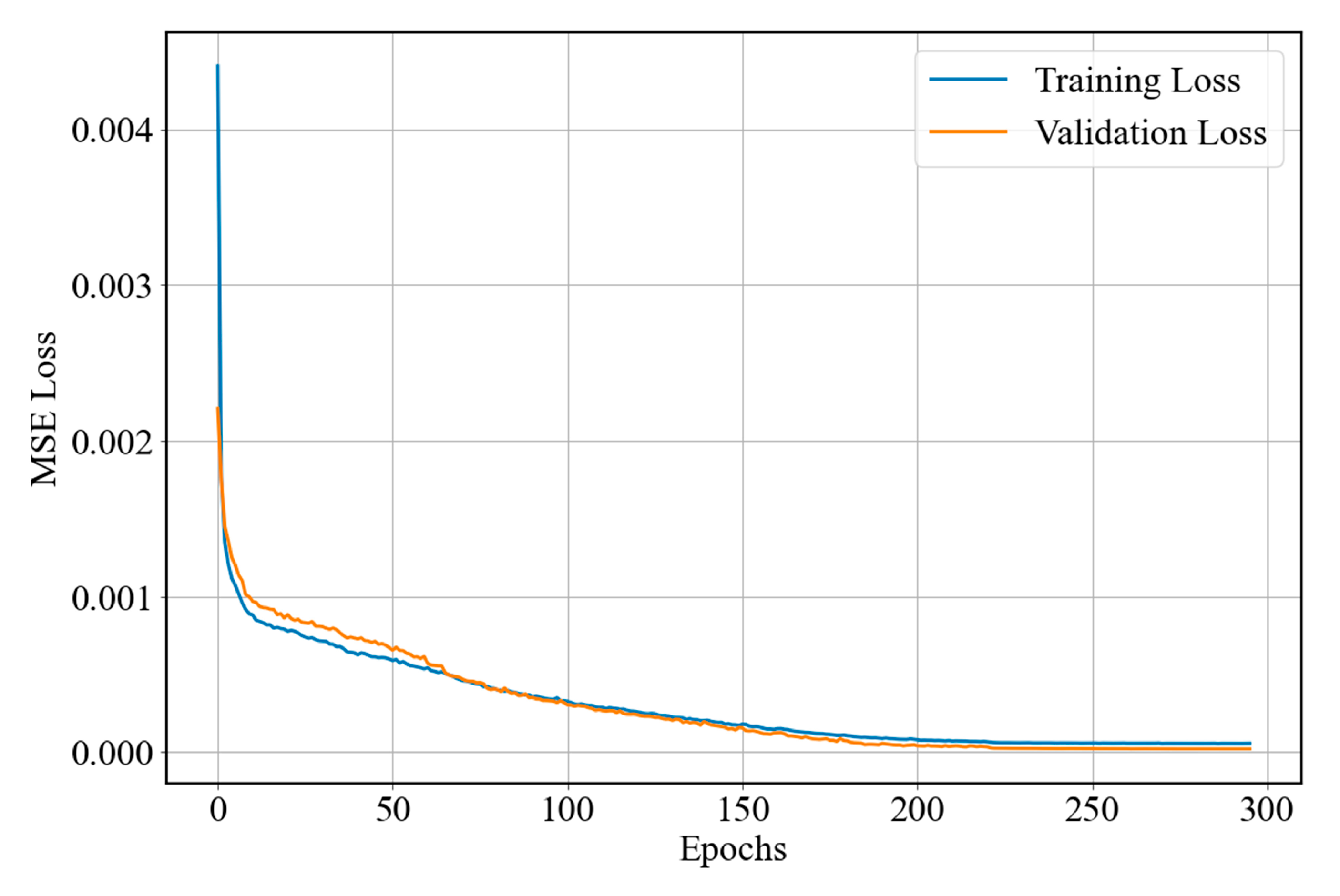
	Output	Squeeze	(B, 512)

, respectively. The optimal hyperparameters are determined based on the reconstruction loss during validation through the use of the grid search algorithm. The model was trained using AdamW as the optimizer for up to 400 epochs, with early stopping employed to avoid overfitting by halting training when the validation loss ceased to improve. The training and validation losses with the optimized parameters are shown in Figure 5. The computational work was done on a computer in PyTorch with an i5 12400F CPU, an NVIDIA RTX3060 GPU, and 16GB of RAM.

3.3. HI Construction and FPT Detection

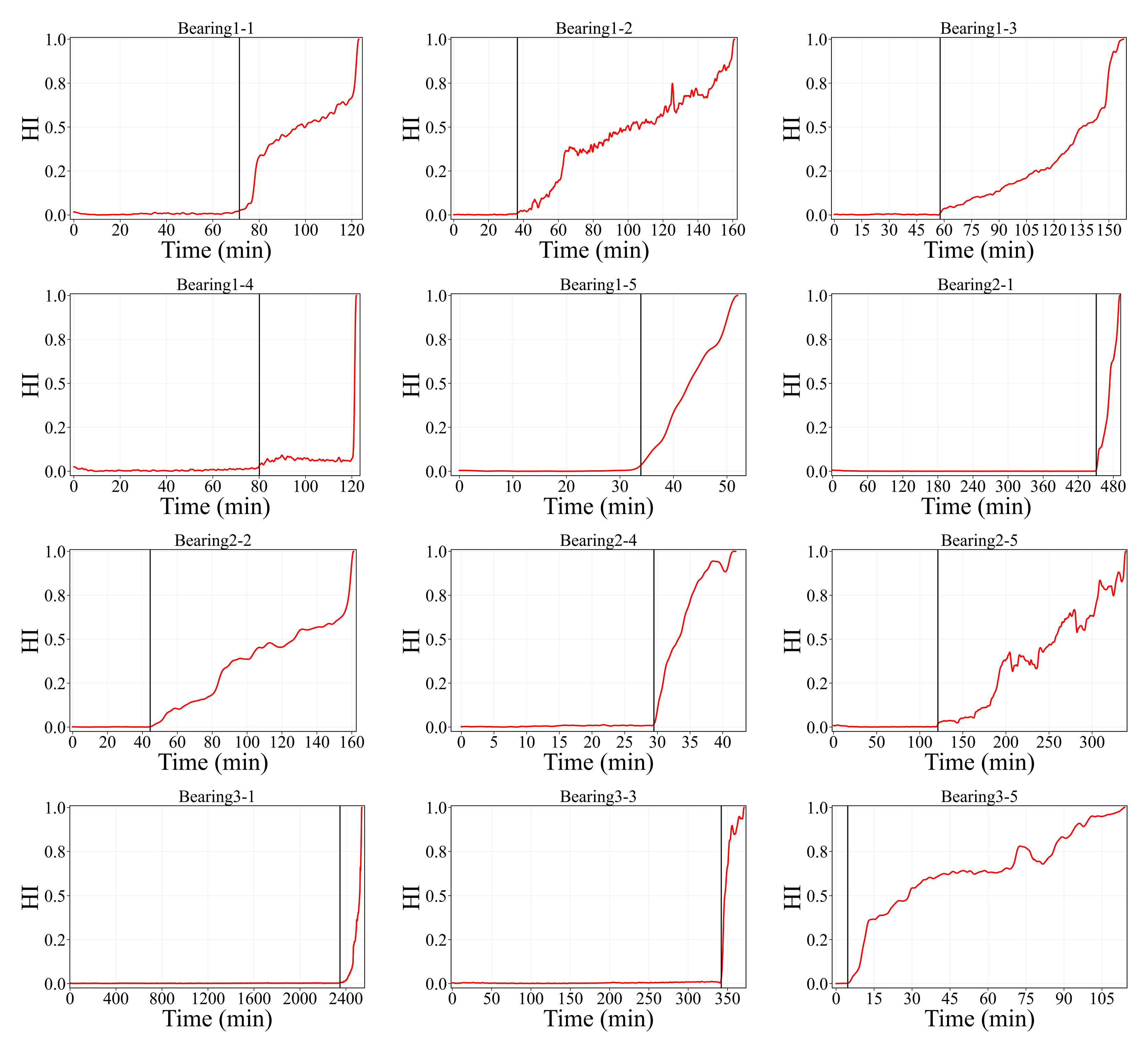
The HCVT-WD model was used to construct the HI for all bearings under various operating conditions. These indicators display a clear trend over time, which is crucial for FPT detection and RUL prediction. To further enhance the clarity of these indicators, Gaussian smoothing was applied to the raw HI as shown in Figure 6, effectively filtering out noise while preserving the overall degradation trend. The smoothed curves provide a more stable and interpretable representation of bearing degradation, facilitating reliable FPT detection and RUL estimation. The FPT and corresponding HIs for the bearings are illustrated in Figure 7.

3.4. Evaluation Metrics of HIs

This study presents three quantitative metrics: monotonicity (Mo), trendability (Tr), and prognosability (Pr) to evaluate the effectiveness of HI construction, as defined in Equations (1)–(3):

$$\mathrm{M}\mathrm{o}=\left|1-{{\displaystyle \frac{6{\displaystyle {\sum }_{\mathrm{j}=1}^{\mathrm{N}}({\mathrm{P}}_{\mathrm{j}}-\mathrm{j})}}{\mathrm{N}({\mathrm{N}}^2-1)}}}^2\right|$$

(27)

$$\mathrm{T}\mathrm{r}\mathrm{e}={\displaystyle \frac{\left|\mathrm{N}{\displaystyle {\sum }_{\mathrm{j}=1}^{\mathrm{N}}\left(\mathrm{H}{\mathrm{I}}_{\mathrm{j}}{\mathrm{t}}_{\mathrm{j}}\right)-\left({\displaystyle {\sum }_{\mathrm{j}=1}^{\mathrm{N}}\mathrm{H}{\mathrm{I}}_{\mathrm{j}}}\right)\left({\displaystyle {\sum }_{\mathrm{j}=1}^{\mathrm{N}}{\mathrm{t}}_{\mathrm{j}}}\right)}\right|}{\sqrt{\left[\mathrm{N}{\displaystyle {\sum }_{\mathrm{j}=1}^{\mathrm{N}}\mathrm{H}{\mathrm{I}}_{\mathrm{j}}^2}-{\left({\displaystyle {\sum }_{\mathrm{j}=1}^{\mathrm{N}}\mathrm{H}{\mathrm{I}}_{\mathrm{j}}}\right)}^2\right]\left[\mathrm{N}{\displaystyle {\sum }_{\mathrm{j}=1}^{\mathrm{N}}{\mathrm{t}}_{\mathrm{j}}^2}-{\left({\displaystyle {\sum }_{\mathrm{j}=1}^{\mathrm{N}}{\mathrm{t}}_{\mathrm{j}}}\right)}^2\right]}}}$$

(28)

$$\mathrm{Pr}=\exp \left(-{\displaystyle \frac{{\mathrm{\sigma }}_{\mathrm{H}{\mathrm{I}}_{\mathrm{f}}}}{\left|{\mathrm{\mu }}_{\mathrm{H}{\mathrm{I}}_{\mathrm{i}}}-{\mathrm{\mu }}_{\mathrm{H}{\mathrm{I}}_{\mathrm{f}}}\right|}}\right)$$

(29)

where ${\mathrm{P}}_{\mathrm{j}}$ represents the rank of the j-th HI within the HI sequence and $\mathrm{N}$ denotes the number of samples. $\mathrm{H}{\mathrm{I}}_{\mathrm{j}}$ is the value of the HI at the time ${\mathrm{t}}_{\mathrm{j}}$. ${\mathrm{\mu }}_{\mathrm{H}{\mathrm{I}}_{\mathrm{i}}}$ and ${\mathrm{\mu }}_{\mathrm{H}{\mathrm{I}}_{\mathrm{f}}}$ denote the means of the HI values at the initial and failure phases, and ${\mathrm{\sigma }}_{\mathrm{H}{\mathrm{I}}_{\mathrm{f}}}$ is the standard deviation of the HI values in the failure phase. All three evaluation metrics range between 0 and 1, with values closer to 1 indicating higher-quality health indicators that exhibit more consistent degradation trends, stronger linear relationships with time, and more predictable failure behavior.

To validate the effectiveness of the proposed method, we compared its performance against three state-of-the-art HI construction methods: ensemble stacked autoencoder (ES-AE), deep CNN-auto-encoder–decoder (DCN-AE), and multi-scale CNN-auto-encoder–decoder (MSC-AE), using the aforementioned evaluation metrics. As shown in Figure 8 and

Table 5. Evaluation results of HI.

Model	Monotonicity	Trendability	Prognosability
ES-AE [37]	0.8415	0.7726	0.8657
DCN-AE [38]	0.9238	0.8188	0.8908
MSC-AE [25]	0.9319	0.8279	0.8898
HCVT-WD (Proposed)	0.9742	0.9376	0.9673

, our method consistently outperforms the other approaches across all evaluation metrics.

While ES-AE is capable of capturing the overall degradation trend, it suffers from noise, which lowers both monotonicity and trendability. DCN-AE and MSC-AE demonstrate better performance by leveraging convolutional feature extraction and multi-scale representations, yet their HIs still exhibit noticeable fluctuations, particularly in the mid-life regions. In contrast, the proposed HCVT-WD achieves superior results through a dual-branch design: the CNN branch effectively filters out local noise from raw vibration signals, while the Vi-T branch captures long-range dependencies and global structural information. The integration of these two branches through skip fusion produces smoother HI curves with reduced oscillations, which explains the markedly higher monotonicity, trendability, and prognosability observed for HCVT-WD.

3.5. Visualization Analysis

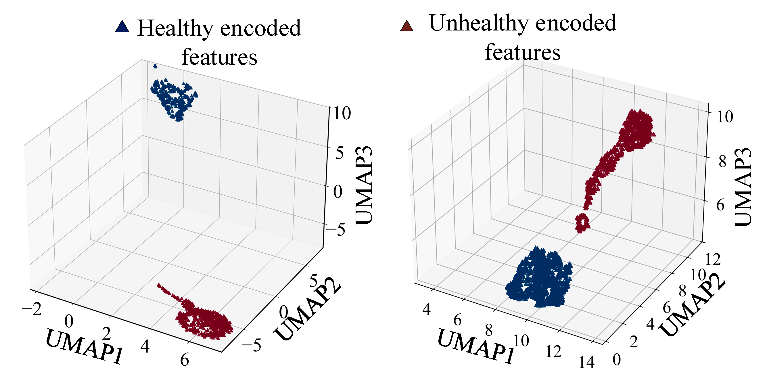
In the visualization analysis, the healthy and degraded features are clearly separated in the uniform manifold approximation and projection embedding space, even when testing with full healthy and degraded samples, as shown in Figure 9. This separation indicates that the proposed HCVT-WD model effectively segregates the encoded features. Notably, the unhealthy features follow a clear degradation trajectory in the embedding space, reflecting the progressive failure process, while the healthy features remain well clustered. This separation is attributed to the multi-head self-attention mechanism in the Transformer, which enhances discriminative feature learning. The attention maps further validate this behavior, as illustrated in Figure 10, where the learned attention weights for three randomly selected testing samples exhibit sparsity in the attention matrices. This sparsity confirms that the proposed module successfully captures dynamic and temporal dependencies within the raw input signals, thereby improving the model’s cycle life prediction capability by focusing on the most informative features.

3.6. RUL Estimation and Uncertainty Analysis

The CNN-Bi-LSTM model, integrated with a Bayesian neural network, was employed to map the HIs to the RUL. To predict the RUL for each bearing, the FPT was initially identified. After determining the FPT, post-FPT HI values were collected, and RUL labels were assigned. These labels indicate the remaining life as a percentage of the total remaining time after the FPT for each bearing.

The samples were created by looking at sequences of 10 consecutive time steps of the HIs. Each sequence consisted of a sliding window of 10 time steps, and the model used these sequences to learn how the health of the bearing evolves over time. Once the sequences were created, the data were randomly split into training and validation sets, with 80% used for training and 20% used for validation. For each sequence, the RUL label was assigned based on the remaining life at the end of the sequence.

During the training phase, a leave-one-out cross-validation method was used for each operating condition. For each bearing, one was held out as the test set, while the others under the same operating condition were used to train the model. To evaluate the proposed method’s accuracy, two performance metrics—RMSE and MAE—were used. These metrics were calculated as follows:

$$\mathrm{R}\mathrm{M}\mathrm{S}\mathrm{E}=\sqrt{{\displaystyle \frac{1}{\mathrm{n}}}{\displaystyle \sum _{\mathrm{t}=1}^{\mathrm{n}}{(\mathrm{y}-\widehat{\mathrm{y}})}^2}}$$

(30)

$$\mathrm{M}\mathrm{A}\mathrm{E}={\displaystyle \frac{1}{\mathrm{n}}}{\displaystyle \sum _{\mathrm{t}=1}^{\mathrm{n}}|\mathrm{y}-\widehat{\mathrm{y}}|}$$

(31)

where $\mathrm{y}$ and $\widehat{\mathrm{y}}$ represent the actual and predicted RUL values, respectively, and $\mathrm{n}$ is the total number of samples.

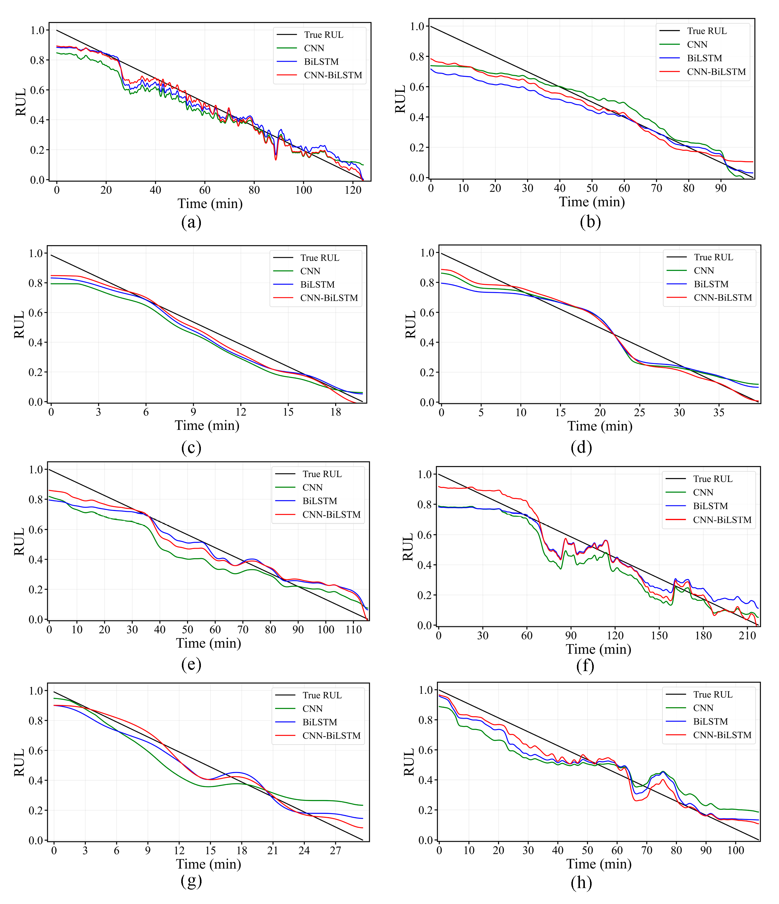
The hyperparameters of the proposed model were carefully tuned, with the optimized values being a batch size of 32, a learning rate of 0.0001, and two LSTM hidden layers with 64 and 32 neurons. A dropout was added after the first hidden layer, and an additional dropout of 0.3 was applied after the final FC layer to implement MC dropout for uncertainty estimation. The prediction results of the proposed methodology are shown in Figure 11 across different working conditions. Additionally, separate CNN and Bi-LSTM prediction networks were constructed for comparison, and the results are presented in

Table 6. Performance comparisons of different models.

Models	Metrics	Test Bearings
		B1-2	B1-3	B1-5	B2-1	B2-2	B2-5	B3-3	B3-5
CNN	MAE	0.0491	0.0713	0.0502	0.0601	0.0906	0.0873	0.0859	0.1078
	RMSE	0.0616	0.0892	0.0605	0.0708	0.1147	0.1071	0.1066	0.1196
Bi-LSTM	MAE	0.0461	0.1075	0.0738	0.0659	0.0706	0.0709	0.0562	0.0843
	RMSE	0.0573	0.1184	0.0822	0.0812	0.0874	0.0876	0.0632	0.0942
CNN-BiLSTM	MAE	0.0321	0.0713	0.0391	0.0463	0.0652	0.0527	0.0374	0.0521
	RMSE	0.0441	0.0887	0.0477	0.0564	0.0758	0.0667	0.0459	0.0639

. The performance comparison demonstrates that the CNN-Bi-LSTM model outperforms these alternatives, achieving superior accuracy in RUL prediction.

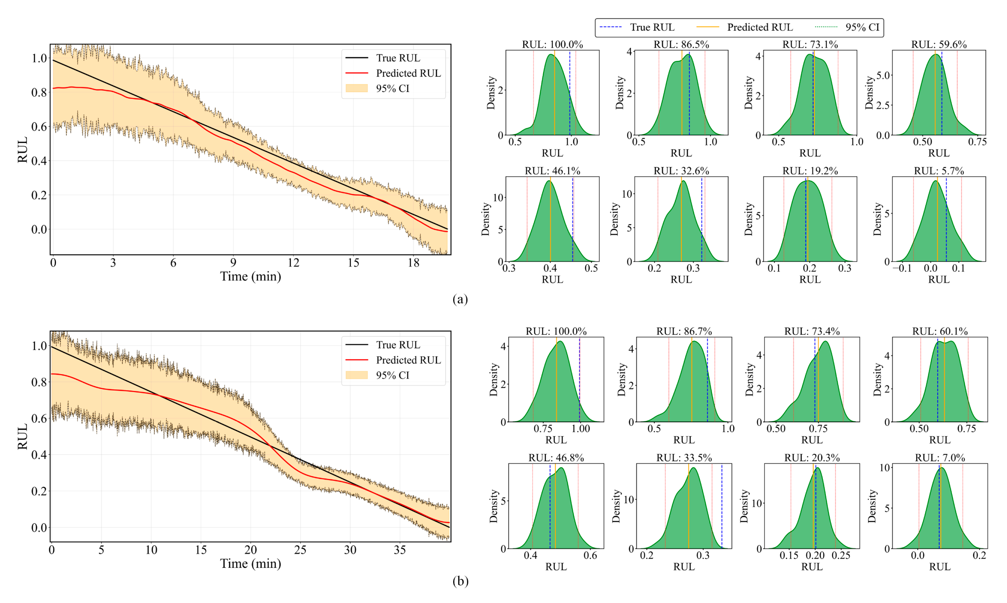
For uncertainty quantification, an MC dropout rate of 0.3 was applied during inference. Additionally, prediction uncertainty was quantified through statistically derived confidence intervals, as shown in Figure 12. Notably, all RUL predictions remain within the calculated 95% confidence bounds throughout the degradation process. KDE analysis revealed that the predicted RUL distributions are tightly clustered around the true values, with minimal skewness. This synergy of accurate point estimation and rigorous uncertainty quantification represents a significant advancement for industrial condition-based maintenance, where understanding both the predicted RUL and its associated confidence level is critical for operational decision-making. The consistent outperformance of conventional approaches validates the efficiency of merging convolutional feature extraction with sequential pattern identification in this integrated prognostic framework.

3.7. Ablation Studies on the HCVT-WD Model

This ablation study investigates the impact of CNN patch embedding, varying patch sizes, and skip connection fusion. As illustrated in Figure 13a the reconstruction loss, observed through both training and validation losses, remains high, fluctuates significantly, and converges slowly in the absence of CNN patch embedding. This indicates that CNN patch embedding performs effectively via convolution operations, and highlights the critical role of patch embedding. Similarly, for a patch size of 16, the reconstruction loss curves exhibit smoother and more rapid convergence compared to patch sizes 8 and 32, as shown in Figure 13b. Furthermore, the introduction of skip connection fusion after the transformer block, aimed at enhancing feature reusability and preserving spatial information, results in a marked improvement in reconstruction loss, as shown in Figure 13c. The skip connection fusion enables the decoder to leverage both high-level features from the transformer blocks and low-level features from the encoder, leading to more stable and smoother convergence of the loss curves and improving the accuracy of the reconstructed input data.

3.8. Comparative Experiments with Other State-of-the-Art Methods for RUL Prediction

To further validate the usefulness of our developed method, a comparative analysis was conducted with four alternative models: the memory fusion network (CLSTMF) [39], self-adaptive graph convolutional networks with self-attention (SAGCN-SA) [40], Time Transformer convolutional LSTM (TT-ConvLSTM) [41], and TCN-Transformer [42]. The first three models were designed for feature extraction and direct RUL prediction, whereas the TCN-Transformer model adopted a two-stage degradation process, considering both HI construction and RUL mapping.

The CLSTMF model achieved a lowest RMSE of 0.051, while the TT-ConvLSTM model showed the lowest RMSE and MAE values of 0.072 and 0.052, respectively. The TCN-Transformer model performed relatively well with a lowest RMSE of 0.0549 and MAE of 0.0441. In contrast, our proposed two-stage degradation model consistently outperformed most of the alternatives, yielding the lowest RMSE of 0.0441 and MAE of 0.0321, demonstrating superior predictive accuracy across all metrics. These results of the comparative experiments are summarized in

Table 7. Performance comparison of different models.

Test Bearings	CLSTMF	SAGCN-SA	TT-ConvLSTM		TCN-Transformer		Proposed
	RMSE	RMSE	RMSE	MAE	RMSE	MAE	RMSE	MAE
B1-2	0.064	0.079	0.185	0.155	0.0621	0.0512	0.0441	0.0321
B1-3	0.181	0.123	0.101	0.062	0.0748	0.0625	0.0887	0.0713
B1-5	0.181	0.188	0.072	0.052	0.0572	0.0430	0.0477	0.0391
B2-1	0.051	0.181	0.094	0.079	0.0673	0.0549	0.0564	0.0463
B2-2	0.156	0.244	0.099	0.081	0.0784	0.0621	0.0752	0.0654
B2-5	0.124	0.145	0.101	0.086	0.0549	0.0441	0.0667	0.0527
B3-3	0.156	-	0.143	0.127	0.0632	0.0519	0.0459	0.0374
B3-5	0.144	-	0.199	0.161	0.0733	0.0614	0.0678	0.0521

, where the RMSE and MAE values for each model are provided. This emphasizes the effectiveness of our approach in accurately predicting RUL through the two-stage degradation process, including both point prediction and interval prediction.

4. Conclusions

This study proposed the HCVT-WD framework for constructing HIs in an unsupervised manner and predicting the RUL of bearings. Raw vibration signals are processed by a sequential CNN–vision Transformer architecture, eliminating manual feature engineering while capturing local spatial patterns and long-range temporal dependencies. The HI is defined as the Wasserstein distance between encoded representations of healthy and degraded states, providing a precise metric of degradation severity. Experimental validation on bearing datasets shows that the proposed HI outperforms state-of-the-art methods in monotonicity, trendability, and prognosability. For RUL estimation, the HI is seamlessly integrated into a CNN-BiLSTM regressor that models both temporal and nonlinear degradation dynamics. A Bayesian neural network yields uncertainty-aware predictions and confidence, which support risk-informed maintenance decisions for safety- and mission-critical applications. The HCVT-WD model requires minimal preprocessing and operates without full lifecycle data, making it adaptable to real-world industrial applications. Its capacity to yield robust HIs and quantify predictive uncertainty establishes it as a potent paradigm for PHM in intricate systems.

Future research will prioritize the development of adaptable HIs across varying operational conditions, validated through extensive testing on heterogeneous datasets to broaden their applicability. Additionally, attention will be directed towards addressing the uncertainty present in both the measurement process and the model’s predictions. This includes the integration of measurement uncertainty as well as other sources of uncertainty, such as model and environmental factors, into the development of more robust and reliable predictive models. Furthermore, future work will focus on fault diagnosis and prognosis through HI construction in a dual-task learning framework, with an emphasis on incorporating zero-fault-shot learning techniques to improve the model’s adaptability to unseen fault types and operational conditions.