PRPOS: A Periodicity-Aware Resource Prediction Framework for Online Services

Abstract

Accurate prediction of resource utilization is essential for efficient cloud resource management and Quality-of-Service (QoS) assurance in online services. However, most existing methods neglect to explicitly model inherent periodic patterns in resource usage—particularly those characterized by extended period lengths, consistent trend shapes with significant magnitude variations across periods—which limits their predictive accuracy. To address this gap, we propose PRPOS (Periodicity-aware Resource Prediction for Online Services), a novel periodicity-aware prediction framework specifically designed for online service workloads. PRPOS operates in two cohesive phases: It first employs a robust period detection mechanism that effectively handles magnitude variations and noise to identify dominant periods; then, a dual scale based on a Gated Recurrent Units (GRU) predictor explicitly incorporates the identified periodicity to concurrently model fine-grained in-period dynamics and coarse-grained cross-period trends. Extensive evaluation on the Alibaba Cluster Trace v2018 demonstrates that PRPOS consistently outperforms state-of-the-art approaches, achieving average improvements of 45.3% in Mean Absolute Percentage Error (MAPE) and 44.3% in Root Mean Squared Error (RMSE). The demonstrated performance enables the application of PRPOS to cloud resource orchestration for online services, allowing for proactive resource provisioning that enhances both efficiency and reliability.

1. Introduction

With the rapid development of cloud computing technology, an increasing number of online services, such as web services and stream processing, are being deployed on cloud platforms to harness the unlimited availability of virtualized resources and a pay-as-you-go cost model [1]. Efficient resource provisioning is crucial to guarantee the QoS of online services as well the cloud resource utilizations [2]. However, as the incoming service requests are fluctuating, the resource demands of online services vary constantly over time. Provisioning resources in a dynamic and cost-effective manner presents a significant challenge for cloud operators.

Accurate resource prediction is the premise of dynamic resource provisioning to online services [3]. In cloud scenarios, the resource prediction of online services mainly refers to using their historical resource usage to estimate their future resource utilization. With an accurate resource prediction, cloud operators can make reasonable resource provisioning decisions so as to improve service quality and reduce the waste of cloud resources.

As online services are typically long-running, their resource utilization patterns naturally lend themselves to being conceptualized as time series. Periodicity encapsulates the recurrent pattern of variations observable in such time series. As the scale of services expands and the regularity of users’ service access patterns intensifies, the periodic characteristic gains even greater significance in the resource usage of online services. Our statistical analysis, anchored in the Alibaba cluster trace, reveals that over 90% of online services exhibit distinctive periodic characteristics in their resource usage [4].

Previous studies in resource predictions have not yet to focus on these periodic features of online services. Even when attempts were made to harness the temporal dynamics of online service resource utilization, they frequently assumed that future resource demands are solely correlated with the most recent historical data points. These studies have primarily relied on regression techniques, such as Autoregressive Integrated Moving Average (ARIMA), or machine learning approaches, like Convolutional Neural Networks (CNNs) and attention mechanisms, to implicitly explore correlations between resource usage at different time points [4,5,6,7,8,9,10,11]. However, our statistical analysis has unveiled that online service resource utilization exhibits long-term periodic patterns. For instance, in the Alibaba cluster trace, the period length of resource usage for approximately 50% of online services exceeds 800 consecutive data points. However, current approaches to resource prediction typically utilize no more than 30 of the most recent data points [12,13,14]. Merely relying on the most proximal historical data points for resource predictions neglects the opportunity to capture cross-period correlations in resource utilization, thereby compromising the accuracy of resource prediction models.

Where promising, periodicity-based resource prediction for online services confronts two fundamental challenges. The first arises in period detection, where dynamic operating environments produce resource usage patterns that simultaneously display trend consistency and magnitude heterogeneity across cycles. Although morphological similarity across cycles confirms consistent periodic behavior, significant variations in both absolute magnitudes (e.g., 15% differences in peak Central Processing Unit (CPU) utilization in Alibaba cluster trace) and oscillatory ranges (e.g., 10-percentage-point amplitude fluctuations in Alibaba cluster trace) undermine the effectiveness of conventional detection methods. Frequency-domain approaches like Fourier transform fail to capture long-term periods due to spectral leakage [15,16,17], while time-domain methods, like auto-correlation analysis, are oversensitive to amplitude variations and suffer from peak submergence [18,19]. Although advanced time–frequency joint methods improve accuracy through multi-level wavelet decomposition, their high computational complexity fails to meet the lightweight real-time detection requirements of online services [20,21].

The second challenge lies in the inherent shortcomings of conventional predictive modeling. Most existing approaches, including advanced deep learning methods, employ a single-scale architecture to process resource usage data—a complex mix of long-term periodic patterns and short-term noise [22,23,24]. This unified representation fails to disentangle multi-scale temporal dependencies, causing models (even those with attention mechanisms) to struggle in distinguishing structurally relevant historical phases from incidental fluctuations. Consequently, without explicit mechanisms to capture periodicity, they often assign misplaced attention to recent outliers or noise while underutilizing stable, recurring periodic patterns, ultimately leading to sub-optimal prediction accuracy and robustness in online service resource prediction.

Aiming at addressing the above issues, we propose PRPOS, a novel resource prediction method for online services based on periodicity. PRPOS follows a two-phase framework. In the first phase, termed period detection, we target long-period patterns characterized by consistent trends yet significant magnitude variations. A lightweight detection mechanism is designed, combining normalized and weighted Hodrick–Prescott (HP) [25] filtering with a rank-based Auto-Correlation Function (ACF) [26] to smooth trend variations while preserving temporal order, thereby effectively suppressing magnitude fluctuations and generating a candidate period. Subsequently, a period refinement strategy based on cosine similarity is introduced to validate and adjust the candidate by measuring morphological consistency across different periodic segments, ultimately producing a high-precision period value.

In the second phase, referred to as resource prediction, we propose a periodicity-aware prediction model based on Gated Recurrent Units (GRUs), explicitly designed to leverage the periodic patterns identified earlier. The model comprises three specialized modules—in-period-GRU, cross-period-GRU, and aggre-FCN—which jointly capture both short-term dynamics and long-term periodic characteristics in online service resource usage. Using the pre-detected period length, the in-period-GRU encodes the most recent period to model short-term dynamics, while the cross-period-GRU integrates historical segments aligned with the same phase across multiple cycles to extract stable periodic patterns. The outputs from both GRU modules are then integrated by aggre-FCN, a fully connected network that performs adaptive feature fusion to produce the final prediction. This multi-scale modeling approach effectively exploits periodic structures in resource usage data, enhancing prediction accuracy and robustness in dynamic cloud environments.

The main contribution of this paper can be summarized as follows:

• A proposal for incorporating periodicity characteristics into resource usage prediction for online services in cloud data centers.
• A novel two-phased online service resource prediction framework, i.e., PRPOS. It accurately identifies dominant periods through a hybrid detection mechanism capable of handling significant magnitude variations across cycles. It also introduces a dual-scale GRU-based predictor that explicitly utilizes the discovered periodicity to simultaneously capture fine-grained in-period patterns and coarse-grained cross-period trends.
• A comprehensive evaluation of PRPOS against other state-of-art baselines. Extensive experiments based on real-world and synthetic datasets confirm its significant improvements in prediction accuracy and robustness, solidifying its practical value for resource prediction in cloud environments.

The rest of this paper is organized as follows. We discuss the related works of this research in Section 2. We provide a detailed description of PRPOS in Section 3. Performance evaluation results are presented in Section 4. Discussion of our work is provided in Section 5. Finally, we conclude our work in Section 6.

2. Related Works

2.1. Resource Prediction

To maximize the utilization of shared resources, accurate resource prediction has become critical in data centers. It not only helps reduce resource waste effectively but also ensures QoS. Existing resource prediction approaches can be broadly categorized into three types: statistical methods, machine learning-based methods, and deep learning-based methods.

Statistical methods: Calheiros et al. [5] developed an ARIMA-based module for cloud workload prediction. Bi et al. [6] proposed a hybrid method that combines wavelet decomposition and ARIMA to predict the number of arriving tasks at the next time interval in data centers. Chen et al. [27] used Ensemble Empirical Mode Decomposition (EEMD) to decompose the time series, predicted each component separately with ARIMA, and combined the results to estimate host utilization. Sharifian et al. [28] applied a three-level wavelet decomposition to the original series, predicted trend and low-frequency components with SVR, and modeled high-frequency components with a Generalized AutoRegressive Conditional Heteroskedasticity(GARCH) model. However, these statistical methods rely heavily on prior knowledge of data characteristics such as distribution and trends, demanding considerable domain expertise. They also generally perform poorly on nonlinear or non-stationary data.

Machine learning-based methods: Such methods do not require extensive prior knowledge and are therefore widely used in handling nonlinear and non-stationary data problems [29,30,31]. Moreno-Vozmediano et al. [7] used a Support Vector Machine (SVM) regression model, whose parameters were selected by an analytical method, to predict the workload of the web server based on historical observations. Baig et al. [32] proposed a novel method to adaptively and automatically identify the most appropriate model to accurately predict data centers’ resource utilization. Gao et al. [33] introduced a clustering-based workload prediction method, which first clusters all the tasks into several categories and then trains a prediction model for each category respectively. Wen et al. [34] presented a Deep Belief Network (DBN) and Particle Swarm Optimization (PSO)-based CPU usage prediction algorithm named DP-CUPA and aimed to provide more accurate CPU usage prediction in data centers. Chen et al. [35] proposed a new Memory Wavelet Neural Network (MWNN) model to achieve both high accuracy and low time consumption in the prediction of real-time data streams. Xiao et al. [8] proposed Enhanced Extreme Gradient Boosting (Enhanced-XGB), an XGBoost-based prediction model, which integrates a convolutional neural network to train the weights of each tree. The final prediction is obtained through a weighted sum of the individual tree predictions plus a bias term. The common drawback of such methods lies in their failure to fully leverage the dynamic dependencies embedded in historical data along the temporal dimension.

Deep learning-based methods: Such methods can effectively capture complex patterns in historical data and achieve higher prediction accuracy. Zhang et al. [9] used Recurrent Neural Networks (RNN) for workload prediction, while Song et al. [10] applied Long Short-term Memory (LSTM) for multi-step-ahead workload predictions. H. M. Nguyen et al. [36] introduced an LSTM Encoder–Decoder model to enhance memory capability. Thonglek et al. [37] designed an LSTM-based model to improve resource allocation decisions for batch jobs. Shen et al. [38] proposed a host load prediction model using bidirectional LSTM (BiLSTM), and Bi et al. [12] combined bidirectional and grid LSTM networks for high-quality predictions of workload and resource series. Surbab et al. [13] developed a deep learning approach with adaptive window size selection to capture recent resource utilization trends. Ouhame et al. [39] employed a CNN-LSTM model to predict multivariate workload (CPU, memory, and network usage). Shu et al. [14] designed an attention-based GRU model to efficiently extract valuable information from large datasets. Chen et al. [40] proposed Resource Prediction based on Temporal Convolutional Networks (RPTCN), a Temporal Convolutional Network (TCN) to capture the long-term temporal dependencies for resource usage prediction. J. Dogani et al. [41] combined CNN and GRU to improve multi-step host workload forecasting. J. Bi et al. [11] integrated multi-head attention with hybrid LSTM for accurate workload and resource prediction. S. Garg et al. [22] developed a deep learning model incorporating BIRCH clustering with LSTM, Transformer, and Informer architectures to predict resource utilization in heterogeneous clouds. H. Yuan et al. [23] introduced VSBG, a prediction approach that combines Variational Mode Decomposition (VMD), Savitzky Golay (SG) filter, BiLSTM, and Grid LSTM, for precise workload and resource predicting in data centers. F. Ullah et al. [42] designed a BiLSTM-based framework for predicting nonlinear multivariate workload and resource utilization. Lastly, S. Tripathi et al. [24] proposed MWRP, a novel architecture integrating Transformer, CNN, and LSTM to improve environmental resource utilization prediction in cloud computing. S. Kashyap et al. [43] introduced a Variable-Size Sliding Window (VSSW) and a Model Selector Decision Support System (MSDSS), this is an approach for multi-model methods, incorporating ARIMA, Multiple Linear Regression (MLR), Gaussian Process Regression (GPR), Multi-Layer Perceptron (MLP), Support Vector Machine Regression (SVMR), and LSTM. However, this approach has two notable limitations: It relies on manual threshold tuning for model selection and lacks a mechanism for explicit periodicity modeling. J. bi et al. [44] proposed a forecasting method based on the Integration of a SG filter, a Frequency-Enhanced Decomposed Transformer (FEDformer) model, and a Frequency-Enhanced Channel Attention Mechanism (FECAM), named FISFA. FISFA converts raw time-series data into the frequency domain to enhance robustness in long-sequence forecasting. Its proposed FEDformer module replaces the standard Transformer to capture multi-scale dependencies with lower computational complexity. However, the method still relies on a deep architecture that incurs significant costs, and its implicit frequency-domain approach fails to explicitly model temporal periodicity.

In summary, existing deep learning-based prediction methods primarily focus on implicitly capturing temporal dependencies in long sequences of resource usage, while overlooking inherent periodic patterns. This failure to explicitly leverage such characteristics for selecting highly relevant historical data not only reduces prediction accuracy but also increases model training complexity.

2.2. Period Detection

Existing periodicity detection algorithms can be broadly classified into two categories: (1) time-domain methods, which identify periodic patterns by analyzing the signal’s self-similarity using the ACF [18,19,45]; and (2) frequency-domain methods, which detect underlying periodicities by transforming the time series into the frequency domain via the Discrete Fourier Transform (DFT) [15,16,17,46], producing a periodogram that represents energy distribution across frequencies. However, ACF-based approaches are sensitive to outliers and noise, often resulting in false alarms, while periodograms suffer from spectral leakage [47], leading to inaccurate or coarse period estimates—especially for long periods.

To mitigate these issues, a number of hybrid methodologies operating in both time and frequency domains have been developed. For instance, AUTOPERIOD [47,48] first extracts a set of candidate periods from the periodogram and subsequently validates them by examining corresponding peaks in the ACF, under the assumption that legitimate periods manifest as prominent ACF hills. Spectral and Average Autocorrelation Zero Distance Density (SAZED) [49], as an ensemble approach, combines spectral density estimation from the frequency domain with autocorrelation zero analysis in the time domain, reinforced through iterative autocorrelation refinement. Another extension [50] employs a sliding window mechanism along with a Kalman filter to adapt to non-stationary time series, though its performance is not universal and it remains vulnerable to outlier corruption. ePeriodicity [51] is designed to explicitly account for uncertainties and noise in periodic signals, delivering provable robustness against incomplete observations, albeit only applicable to binary sequence data. RobustPeriod [20,21] is the state-of-art period detection work. It is a robust multiple periodicity detection framework that decouples intertwined periodicities via Maximal Overlap Discrete Wavelet Transform (MODWT) in the time–frequency domain, and it leverages a robust Huber-periodogram and Huber-autocorrelation function for detection and validation. Q. Wu et al. [52] introduced a periodic pyramid structure that integrates self-attention with multi-scale periodic modeling to capture complex periodic dependencies in time series, achieving strong performance in forecasting and classification tasks. However, it suffers from high computational cost and limited generalization to weakly periodic or non-periodic data.

In the context of online service resource usage in data centers, periodic behaviors often exhibit extended cycle lengths, consistent trend pattern across cycles as well as non-stationary magnitude variations and contaminations such as noise and outliers. Despite advances in hybrid time-frequency methods, current period detection techniques still fall short in fully addressing these complex characteristics, particularly the high computational complexity, underscoring the need for more robust and efficient solutions tailored to this specific domain.

3. Materials and Methods

3.1. Overview of PRPOS

As illustrated in Figure 1, PRPOS adopts a two-phase framework designed for resource prediction in online services. The framework begins by collecting raw resource usage sequence data—such as CPU utilization of online services—from data center infrastructures. In the first phase, targeting the common characteristics of trend consistency and magnitude variations across multiple periods in resource usage, a period detection method combining normalized HP filtering [25], rank-based ACF [53,54], and cosine similarity [55] is employed. This approach accurately identifies the dominant periodic pattern in the resource sequences through candidate period generation and period refinement steps. In the second phase, leveraging the detected periodic structure, PRPOS constructs a prediction model capable of integrating multi-period temporal features. Built around GRUs and Fully Connected Networks (FCNs) [56], the model captures short-term dependencies from recent data (within the current period) and long-term evolutionary patterns from multiple historical periods. Finally, the multi-scale temporal representations are merged through a feature aggregation network to produce accurate predictions of resource usage.

3.2. Period Detection

Period detection in online service resource usage comprises two sequential phases: candidate period detection and period refinement, shown in Figure 2. The candidate period detection phase preserves periodicity through trend decomposition: The original sequence is separated into trend and residual components, with periodic features extracted from residuals to derive preliminary candidates. The refinement phase measures trend similarity between sub-sequences to fine-tune candidates, suppressing spurious patterns caused by magnitude variations and noise while enhancing true periodicity.

3.2.1. Candidate Period Detection

Candidate detection combines HP filtering for cyclical component extraction and rank ACF for period detection.

• Normalized-Weighted HP Filtering-Based Cyclic Component Extraction

The HP filter decomposes the original resource usage sequence Y into trend (${\tau }_t$) and cyclical ($c_t$) components through the canonical formulation $y_t={\tau }_t+c_t$, where $c_t$ provides purified periodic constituents for subsequent period detection [57]. To enhance robustness against magnitude heterogeneity—i.e., variations in overall resource usage levels across periods—while preserving inter-period trend similarity, we introduce a normalized–weighted adaptation of the HP filter.

More specifically, the proposed method initially performs magnitude normalization as follows:

$${\tilde{Y}}_t={\displaystyle \frac{Y_t-{\mu }_Y}{{\sigma }_Y}}$$

(1)

where ${\mu }_Y$ represents the mean of the sequence, and ${\sigma }_Y$ denotes the standard deviation of the sequence.

Subsequently, for the normalized sequence, weights are calculated based on the magnitude of each normalized value using the following formula:

$${\omega }_t={\displaystyle \frac{1}{1+{\tilde{Y}}_t}}$$

(2)

Finally, the HP filter’s objective function is modified as follows:

$$\widehat{\widetilde{c_t}}=\underset{\tilde{c}}{argmin}{\displaystyle \frac{1}{2}}\sum _{\mathrm{t}=0}^{\mathrm{T}-1}{\tilde{c}}_t^2+\lambda \sum _{t=1}^{T-1}{\omega }_t{\left(\left({\tilde{Y}}_{t-1}-{\tilde{c}}_{t-1}\right)-2\left({\tilde{Y}}_t-{\tilde{c}}_t\right)+\left({\tilde{Y}}_{t+1}-{\tilde{c}}_{t+1}\right)\right)}^2$$

(3)

By normalizing the resource usage sequence to eliminate scale dependence and integrating magnitude-dependent weights (${\omega }_t$) into the smoothing constraints, this formulation explicitly addresses magnitude disparities [58]. Here, $\lambda$ is tuned via residual statistical matching. The approach simultaneously suppresses the dominance of cycles with high absolute usage levels and preserves inter-cycle trend similarity, a dual mechanism critical for robust period detection in sequences with variable magnitude.

2.

Candidate Period Detection with Rank-Based ACF

Given the long-period characteristics of online service resource usage, we employ time-domain methods for period detection. While traditional ACF is commonly used [18,19], it fails to reliably identify periods in these sequences due to magnitude variations between cycles—even when they share similar trend patterns. To overcome this limitation, we adopt rank-based ACF, which first transforms the HP-filtered cyclical components into normalized ranks, preserving waveform ordering while eliminating magnitude effects.

For the rank transformation of HP-filtered cyclical components $c_t$, $t\in \{1,2,\dots ,T\}$, we define the rank of any element $c_t$ as follows:

$$r_t=\sum _{i=1}^{T}II\left(c_i<c_t\right)+{\displaystyle \frac{1}{2}}\left(\sum _{i=1}^{T}II\left(c_i=c_t\right)+1\right)$$

(4)

where $II(·)$ denotes the indicator function [59]. The second term handles tied values by assigning average ranks.

Subsequently, we normalize the ranks to the interval [−1, 1] via

$$n{r}_t^{\prime }={\displaystyle \frac{2(r_t-0.5)}{T}}-1$$

(5)

This approach calculates auto-correlation on rank-transformed values rather than raw magnitudes, which completely eliminates inter-cycle magnitude differences while preserving morphological features. By isolating periodicity information from magnitude variations, the results depend solely on waveform similarity, significantly improving robustness in long-period detection for online services.

Based on the normalized rank transformation, we employ Algorithm 1 to compute subsequent periods in online service resource usage.

Algorithm 1 Candidate Period Identification

Input:  Normalized rank sequence of online service resource usage: $NR$ Output:  Candidate period: p   1: $ACFSeq\leftarrow \mathrm{generateACF}\left(NR\right)$ fill // Generate ACF sequence   2: $LocalPeaks\leftarrow \mathrm{findLocPeak}\left(ACFSeq\right)$ fill // Find local peaks   3: $p\leftarrow \mathrm{median}\left(\mathrm{distance}\right(LocalPeaks\left)\right)$ fill // Choose the median distance as period   4: return p

Statistical analysis of Alibaba cluster trace reveals that online service resource usage typically exhibits consistent daily periodic patterns, despite large fluctuations in magnitude. Traditional ACF is highly sensitive to magnitude variations and noise spikes, often requiring error-prone manual threshold tuning. In contrast, Algorithm 1 automatically identifies significant peaks in the auto-correlation of rank-transformed data and determines the period using median peak spacing. This approach eliminates subjective thresholds and reliably detects periods even with strong inter-cycle variations.

3.2.2. Candidate Period Refinement

While our candidate period detection mechanism effectively identifies the candidate period, the preliminary result only indicates possible cycle locations through rank-based ACF peaks without verifying waveform stability in actual resource usage sequences. This necessitates a refinement phase to validate the periodicity through waveform pattern analysis.

The primary principle underlying the period refinement is to partition the original resource usage sequence of online services into several equally sized subsequences, based on the candidate period length, and measure the similarity between these partitioned subsequences. By fine-tuning the candidate period length, we select the one that attains the utmost similarity among the subsequences as the ultimate dominant period.

Considering the value range variations across time periods in online service’s resource usage sequence, we choose cosine similarity as the subsequence similarity measurement. Cosine similarity is commonly employed to gauge the resemblance between two sequences, primarily emphasizing the coherence in their trends rather than their absolute values. A higher cosine similarity value indicates a greater resemblance between the two sequences. For the candidate period, trendSimilarity is defined as the average pairwise cosine similarity among all partitioned subsequences, expressed as

$$trendSimilary={\displaystyle \frac{{\sum }_{k=1,l=1}^{m}cosinesimilarity(X_k,X_l)}{m}},k\ne l$$

(6)

$$cosinesimilarity(X_k,X_l)={\displaystyle \frac{{\sum }_{i=1}^n{x}_i^k·x_i^l}{\sqrt{{\sum }_{i=1}^n{\left(x_i^k\right)}^2}\sqrt{{\sum }_{i=1}^n{\left(x_i^l\right)}^2}}}$$

(7)

where n represents the candidate period length; $X_k$ and $X_l$ respectively represent two different resource usage subsequences; $x_i^k$, $x_i^l$ denote the value of the corresponding points of these two subsequences, $i=1,2\dots n$. The corresponding similarity of each fine-tuned candidate period is expressed as the average of similarity scores among all pairs of subsequences.

The tuning of the candidate period is processed as Algorithm 2.

Algorithm 2 Dominant Period Refinement

Input:  resource usage sequence of online service: $RS$, step size of period refinement: $\Delta t$, terminal condition of period refinement: $sn$; Output:  the ultimate dominant period: $finalCP$   1: $\mathrm{ascCP}\leftarrow 0,\mathrm{decCP}\leftarrow 0,\mathrm{finalCP}\leftarrow 0$ fill // Initialization   2: $\mathrm{ascCP}\leftarrow \mathrm{findascCP}(RS,CP,\Delta t,sn)$ fill // Find candidate period ≥ CP   3: $\mathrm{decCP}\leftarrow \mathrm{finddecCP}(RS,CP,\Delta t,sn)$ fill // Find candidate period ≤ CP   4: $\mathrm{finalCP}\leftarrow \mathrm{compareSimilarity}(\mathrm{ascCP},\mathrm{decCP})$   5: return finalCP

The refinement of the candidate period is based on two underlying assumptions: First, that the candidate period, obtained through the processing of HP and ACF, approximates the eventual dominant period within a few refinement iterations; second, that as the candidate period approaches the ultimate dominant period, the corresponding subsequences display an increasing level of similarity. The refinement process is carried out in two directions, either increasing or decreasing the candidate period by a step size of $\Delta t$. The input $sn$ defines the terminal condition for period refinement. Based on the second assumption, the bidirectional refinement continues until the subsequence similarity shows a continuous decrease over sn consecutive instances (line #2, #3). Once this refinement process is completed, the final dominant period will be chosen from the identified candidate dominant periods in both directions with the higher trend similarity (line #4).

3.3. Resource Prediction

Based on the detected period, PRPOS selectively chooses the relevant historical data to explore the patterns of resource usage variation within and between periods of online services, facilitating accurate resource prediction. In PRPOS, we employ the Gated Recurrent Unit (GRU) neural network as a fundamental component to capture the patterns of variation in resource usage time-series data. These patterns are subsequently combined to generate the final resource prediction.

• Historical Data Selection

Based on the periodic patterns in online service resource usage, we observe that historical data typically contains two components which facilitate the prediction of future demand.

As depicted in Figure 3, the first component, referred to as in-period-data, consists of the resource usage subsequence closest to the prediction time within the most recent period. This component captures short-term dependencies between predicted usage and historical observations. The second component, termed cross-period-data, comprises resource usage subsequences from the same or temporally adjacent points within each historical period relative to the prediction point. This component is essential for two reasons: first, resource usage at corresponding time positions across different periods shows strong similarity; second, incorporating adjacent time points helps represent variation patterns within the value range over periodic intervals. Importantly, this cross-period-data is crucial for modeling long-term dependencies in resource usage behavior.

B.

Model design

Figure 4 demonstrates the resource prediction model in PRPOS.

GRU as Building Block. In designing PRPOS, we deliberately selected Gated Recurrent Unit (GRU) as the fundamental building block for temporal modeling, in preference to more recent alternatives such as Transformer-based architectures. This decision was motivated by several domain-specific considerations. Resource usage in online services (e.g., CPU utilization) is predominantly influenced by immediate past states and, despite the occasional presence of outliers or abrupt changes, typically exhibits smooth and sequential variations rather than arbitrary long-range dependencies. Although Transformers excel at capturing global interactions through self-attention, their quadratic inference complexity makes them less suitable for rapidly updating predictions in resource-constrained, latency-sensitive environments such as online prediction systems. Furthermore, the ability of Transformers to leverage long sequences does not necessarily translate into accuracy gains for online service resource prediction, where recent points and homologous periodic segments carry the most relevant signal.

As shown in Figure 5, with their gated recurrent mechanism, GRUs provide a balanced solution: They mitigate the vanishing gradient problem of simple Recurrent Neural Networks (RNNs) and efficiently model medium-range dependencies while maintaining linear computational complexity and a modest parameter count [9,14]. This makes GRUs particularly well-suited for building lightweight yet expressive temporal feature extractors that can be integrated into larger prediction workflows without introducing unnecessary latency or resource consumption.

Model Architecture. The prediction model in PRPOS is mainly composed of three modules: in-period-GRU, cross-period-GRU, and aggre-FCN.

The in-period-GRU module processes the in-period-data to capture short-term temporal dependencies in resource usage. Specifically, the input is represented as a vector of length w, corresponding to the most recent w time steps within the current period. The vector is processed through a network of GRU units, each handling one time step. These units share parameters, allowing the module to capture sequential dependencies efficiently. The module outputs an m-dimensional feature vector representing the encoded short-term context, where m is a trainable hidden size hyperparameter.

The cross-period-GRU module is designed to capture long-term temporal dependencies from historical resource usage patterns. Its input, the cross-period-data, is structured as a matrix of size $k\times h$, where k denotes the number of historical periods considered and h is the length of the aligned usage subsequence within each period. Each row of the matrix corresponds to a contiguous resource usage subsequence drawn from a historical period. These subsequences are aligned based on the target prediction time—that is, each row starts at the same phase position within its respective period as the current prediction point. The rows are arranged in reverse chronological order, with the most recent period placed first and the earliest period last. Each row is processed independently by a shared GRU unit—that is, the same GRU cell with identical parameters is applied to every row, enabling efficient and consistent feature extraction across all historical sequences. The module ultimately produces an n-dimensional output vector, where n is a learnable hidden size hyperparameter, encoding the long-term temporal features across multiple periods.

The latent representations of both short-term and long-term temporal dependencies—that is, the output vectors from the in-period-GRU and the cross-period-GRU—are concatenated into a unified feature vector. This combined representation serves as the input to the aggre-FCN module. The aggre-FCN consists of a fully connected network that learns to adaptively weight and fuse the short-term and long-term features. Through non-linear transformation and dimensionality reduction, this module effectively synthesizes the multi-scale temporal information to produce the final resource usage prediction.

Model Training. Let the resource usage time series be denoted as $R=\left\{r_t\right\}$ for $0\le t\le n$. Training samples are constructed for each prediction point using an endpoint-based partitioning scheme: We start at time t and extract backward to form contiguous subsequences of length P (the detected period). This approach guarantees that the most recent period—ending exactly at the prediction point—contains a complete set of data points, thereby avoiding truncated or incomplete inputs that would occur if we partitioned from the start of the sequence.

From these period-length subsequences, we derive the two input components. First, the in-period-data comprises the most recent w time steps ending at t. Second, the cross-period-data consists of k segments of length h, each aligned to end at time t across k historical periods. A sample is valid only if at least k historical periods are available. The overall dataset is split chronologically into training and testing sets in a 7:3 ratio. This preserves the temporal order of events and allows us to evaluate the model’s ability to generalize to future time periods, providing a more realistic assessment of its deployment performance. The model is trained to minimize the Mean Squared Error (MSE) [60]:

$$min{\displaystyle \frac{{\sum }_{i=0}^{m-1}{({\stackrel{\wedge }{y}}_i-y_i)}^2}{m}}$$

(8)

In addition, we use the Adam optimizer with learning rate decay, ReLU activations [61], and employ dropout and $L_2$ regularization to mitigate overfitting.

4. Results

In this section, we demonstrate the superior performance of our proposed PRPOS method in resource prediction and period detection using real-world and synthic data center traces. The experimental results are presented graphically in the main text, with the complete numerical data provided in tabular form in Appendix B.

4.1. Experiment Settings

• Datasets

To evaluate the resource prediction capability of PRPOS, we utilize the Alibaba cluster trace v2018 dataset. Released in 2018, this dataset offers comprehensive insights into data center operations by recording the resource usage of over 5000 online services during an eight-day period. Among its six constituent tables, we specifically employ $container\_meta$, which contains service metadata, including the status field used to identify normally functioning services, and $container\_usage$ which includes CPU, memory, and disk measurements recorded at 30-s intervals. After selecting 40 services with normal status from $container\_meta$, we aggregate their resource usage sequences by $container\_id$ in $container\_usage$. 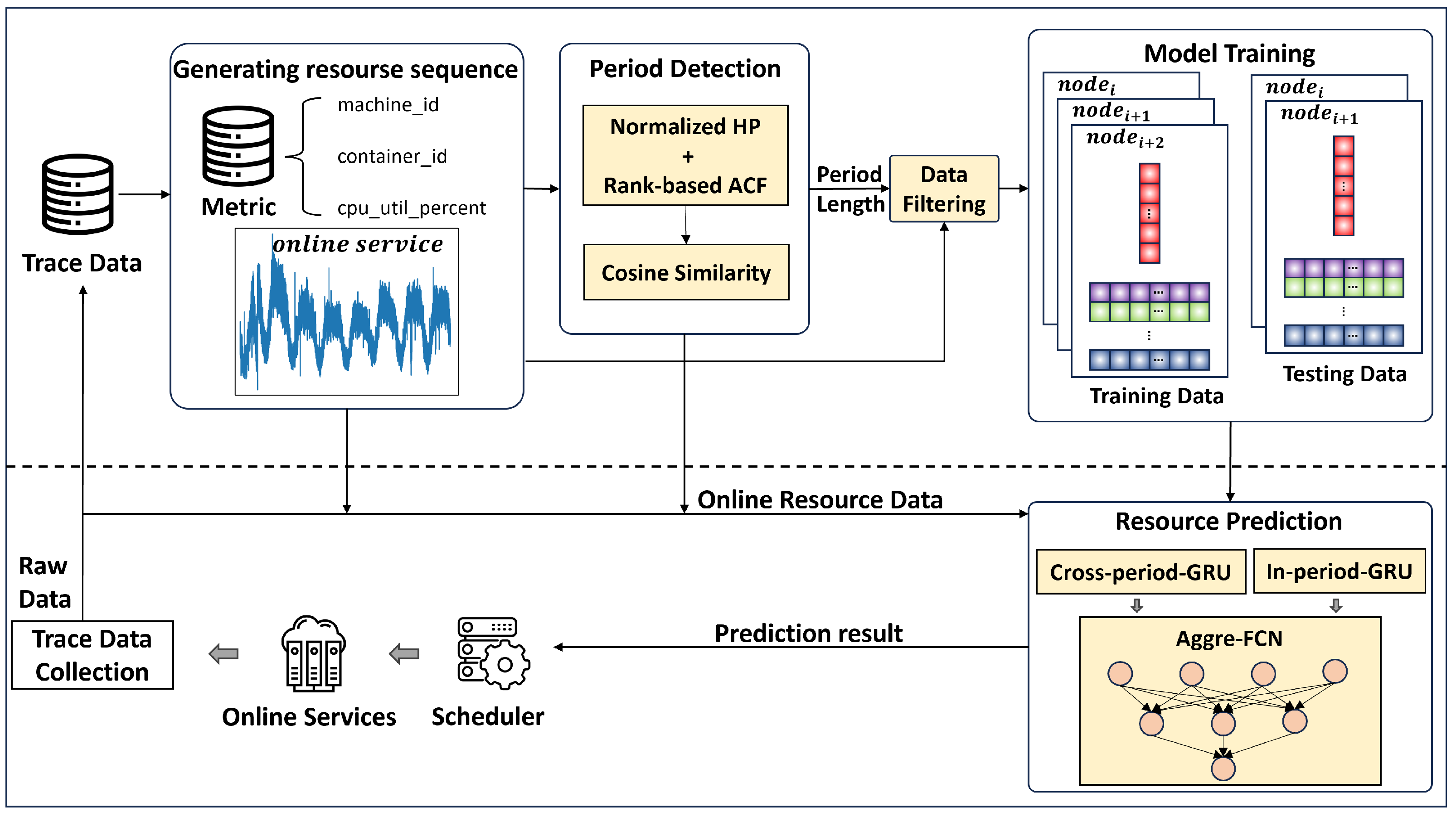We focus on CPU utilization percentage as the primary prediction metric due to its representative nature. For each service, we extract timestamp-sorted CPU utilization percentages to form individual time series, which together constitute our experimental dataset. Each service trains a dedicated resource prediction model using the data partitioning approach described in the "Model Training" subsection in part B of Section 3.3.

To comprehensively evaluate PRPOS’s period detection under scenarios with both trend consistency and magnitude heterogeneity, we construct a synthetic dataset based on statistical characteristics from the Alibaba cluster trace v2018. This dataset enforces trend consistency by maintaining identical resource usage change patterns across consecutive cycles. Periodic patterns are modeled as standard sine waves with period lengths measured in number of 30-s data intervals. The lengths span five ranges—[800–1000), [1000–1200), [1200–1400), [1400–1600), and [1600–1820] intervals—systematically covering the dominant period length distribution in the dataset. For each of the five configurations, we generate 100 CPU usage percentage sequences, each containing 8 cycles. Magnitude heterogeneity is introduced into these sequences through two key dimensions: baseline levels, representing the steady-state resource occupancy and ranging from 5% to 50%, and fluctuation intensity, characterized by ±15% inter-cycle variations. Additionally, we randomly inject Gaussian noise (${\sigma }_n^2=0.1/1/2$) and outliers ($\theta =0.01/0.1/0.2$) into each sequence.

Our experiments are conducted on one server equipped with one 4-core 3.3 GHz Intel Core i5-6600 processor, 32 GB memory, and a 2TB Hard Drive HDD.

B.

Baselines

The experimental baselines were constructed by adapting existing competitive approaches for cloud resource prediction, each employing statistical, machine learning, or deep learning architectures.

• ARIMA [6]: Combines wavelet decomposition and ARIMA for short-term trend prediction but struggles with nonlinear and complex patterns.
• XGBoost [8]: Uses CNN to optimize tree weights, boosting accuracy but increasing computational complexity.
• CNN [62]: Captures local temporal patterns via sliding kernels but fails to model long-term periodic dependencies due to fixed receptive fields.
• LSTM [63]: Robust to noise and temporal dependencies but suffers from high computational complexity and data hunger for intricate patterns.
• BiLSTM [64]: Enhances context modeling with bidirectional processing but inherits LSTM’s high cost and interpretability issues.
• GRU [65]: More parameter-efficient than LSTM but limited in parallelization and long-range dependency modeling.
• GRU+Attention [14]: Attention mechanisms alleviate GRU’s long-range issues but introduce full-sequence processing overhead and noise sensitivity.
• RPTCN [40]: Combines dilated convolutions and attention for long-range dependencies but struggles with periodic phase shifts and irrelevant feature noise.
• VSSW-MSDSS [43]: Dynamically selects among statistical, ML, and DL models via variable-size sliding windows but relies on manual threshold tuning and lacks explicit periodicity modeling.
• FISFA [44]: Leverages SG filter, a FEDformer, and FECAM for spectral patterns, but incurs heavy computation and implicit periodicity handling.

In addition, we evaluate the accuracy and computational efficiency of our period detection method in PRPOS, comparing it to widely adopted frequency-domain and time-domain baselines.

• findFrequency [66]: This is based on using the maximum value in the frequency spectrum to estimate period length.
• SAZED [49]: This approach includes the SAZEDopt and SAZEDmaj variants, which combine spectral and autocorrelation analysis for parameter-free seasonality detection with high efficiency. However, it assumes stable amplitudes and exhibits sensitivity to outliers, owing to its reliance on raw autocorrelation.
• RobustPeriod [20,21]: This leverages wavelet transforms and robust Huber optimization to detect multiple periodicities. It suffers from high computational costs and the phase-amplitude decoupling, making it less ideal for magnitude-varying resource patterns.

C.

Evaluation Metrics

To quantify and compare the prediction performance of PRPOS with the ten baselines, we use two performance metrics—MAPE [67] and RMSE [68]—as follows:

$$MAPE(y_i,y_i^{\prime })={\displaystyle \frac{1}{n}}\sum _{i=1}^n\left|{\displaystyle \frac{y_i^{\prime }-y_i}{y_i}}\right|$$

(9)

$$RMSE(y_i,y_i^{\prime })=\sqrt{{\displaystyle \frac{1}{n}}\sum _{i=1}^n{(y_i^{\prime }-y_i)}^2}$$

(10)

where $y_i$ and $y_i^{\prime }$ are the observed value and ground truth of instance i, and n is the number of all sample instances.

In period detection evaluation, we use Accuracy to measure their performance.

$$Accuracy(y_i,y_i^{\prime })={\displaystyle \frac{1}{n}}\sum _{i=1}^n{\displaystyle \frac{y_i^{\prime }}{y_i}}$$

(11)

D.

Parameter Settings

In this section, we present the core parameter settings in PRPOS. The detailed parameter settings for each baseline model are provided in Appendix A (

Table A1. Parameter settings in baseline methods.

Model	Name	Value
LSTM	Historical observation data window size	60
	Number of hidden units	128
	Batch size	128
	Learning rate	0.005
BiLSTM	Historical observation data window size	60
	Number of hidden units	128
	Batch size	128
	Learning rate	0.001
CNN	Historical observation data window size	60
	Number of convolutional layers	2
	Stride	1
	Kernel size	3
	Learning rate	0.005
RPTCN	Historical observation data window size	60
	Number of convolutional layers	3
	Stride	1
	Kernel size	3
	Learning rate	0.001
	Dilation rates of the three convolutional layers	1, 2, 4
GRU	Historical observation data window size	60
	Number of hidden units	128
	Batch size	64
	Learning rate	0.002
GRU+Attention	Historical observation data window size	60
	Number of hidden units	60
	Batch size	50
	Learning rate	0.001
	Number of attention head	1
	Attention output dimension	60
FISFA	Dimension of model	60
	Learning rate	0.001
	Layer number in encoder	1
	Layer number in decoder	2
	Batch size	16
	Early stopping patience	9

and

Table A2. Parameter settings in VSSW-MSDSS.

Model	Name	Value
ARIMA	p—The order of the autoregressive model	3
	d—The degree of differencing	1
	q—The order of the moving-average model	2
GPR	Kernel function	Radial Basis Function
	Length scale	1.5
	Noise level	0.1
MLR	Regularization parameter	[0.001, 10.0]
MLP	Hidden layers	3
	Neurons per layer	32, 64, 128
	Learning rate	0.001
	Batch size	64
SVMR	Kernel function	Radial Basis Function
	Regularization parameter	1.0
	Gamma	0.1
LSTM	Number of hidden units	128
	Batch size	64
	Learning rate	0.001
MSDSS	Evaluation indicators	True Positive Rate (TPR),
		True Positive Rate (FPR),
		True Negative Rate (TNR),
		False Negative Rate (FNR),
		Accuracy
	Classification methods	Decision tree classifier,
		KNN,
		Naive Bayes

).

The configurable parameters in PRPOS are categorized into three functional groups corresponding to the stages of period detection, sample data selection, and resource prediction modeling. It is noteworthy that the parameters for the prediction modeling stage are specifically the parameters of the deep learning model, as shown in

Table 1. Parameter settings in PRPOS.

	Name	Value
Period Detection	Smoothing parameter in HP filtering ($\lambda$)	14,400
	Rank-based ACF window length (L)	3000
	Rank-based ACF lags (G)	4000
	Cosine similarity threshold ($\tau \_c$)	0.8
	Step size of period refinement ($\Delta t$)	30
	Terminal condition of period refinement ($sn$)	5
Sample Data Selection	Input data size (N)	60
	Sampled window size per cycle (W)	10
	Number of historical cycles (K)	5
Resource Prediction Modeling	Full connection layer depth ($L_{fc}$)	2
	Full connection layer neuron number ($N_{fc}$)	$N_{fc1}$ = 128, $N_{fc2}$ = 64
	GRU hidden unit number ($d_h$)	64
	in-period-GRU hidden layer depth ($L_{ip}$)	1
	cross-period-GRU hidden layer depth ($L_{cp}$)	2
	Learning rate ($\alpha$)	0.005

.

In the period detection stage, the HP filter smoothing parameter ($\mathit{\lambda }$ = 14,400) adopts the classical setting to extract near-daily periodic trends [25]. The rank-based ACF is computed with two key parameters: the window length $\mathit{L}$ and the maximum lag $\mathit{L}$. In our experiments, we set $\mathit{L}$ = 3000 and $\mathit{L}$ = 4000 so as to fully encompass the characteristic near-daily periodicity (6.5–18 h in Alibaba trace) and its potential harmonics of online service CPU usage [26]. The cosine similarity threshold $\mathit{\tau }\_\mathit{c}$ is set to 0.8 to enforce strict waveform consistency against the inherent burstiness and noise in online service CPU usage. During period refinement, the step size $\Delta \mathit{t}$ is set to the minimum sampling interval (30 s) in the trace data to achieve the finest adjustment granularity, while the terminal condition $\mathit{sn}$ is set to 5 to serve as a robust stopping criterion, effectively distinguishing between short-lived noise spikes and a genuine, persistent shift in the periodic pattern of CPU consumption.

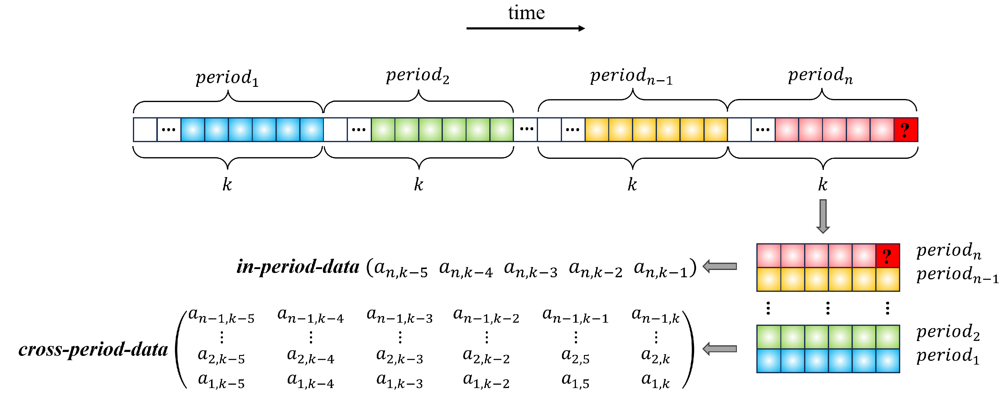
In the sample data selection stage, parameters are set to model the continuous trends and mitigate transient noise in online service’s CPU usage. The input data size $\mathit{N}$ is set to 60 to capture essential short-term context. The sampled window size per cycle $\mathit{W}$ is set to 10 to provide the resolution needed to represent pattern morphology. The number of historical cycles $\mathit{K}$ is set to 5 to offer a robust view of long-term, repeating trends, allowing the model to average out non-repeating noise.

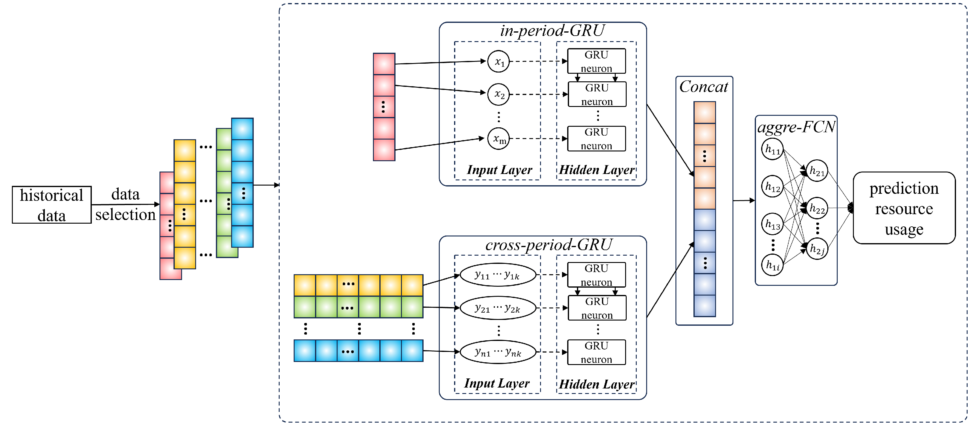
In the resource prediction modeling stage, the model structure is defined by several key parameters. The fully connected network has a depth ${\mathit{L}}_{\mathit{fc}}$ = 2 with neuron numbers ${\mathit{N}}_{\mathit{fc}\mathbf{1}}$ = 128, ${\mathit{N}}_{\mathit{fc}\mathbf{2}}$ = 64, balancing capacity and stability. The GRU hidden unit number ${\mathit{d}}_{\mathit{h}}$ = 64 is chosen for effective temporal modeling. The core design is the dual-scale GRU, where the in-period-GRU hidden layer depth ${\mathit{L}}_{\mathit{ip}}$ = 1 captures high-frequency dynamics, and the cross-period-GRU hidden layer depth ${\mathit{L}}_{\mathit{cp}}$ = 2 models complex long-term trends. The learning rate $\mathit{\alpha }$ = 0.005 ensures stable convergence.

4.2. Results and Analysis

• Overall Performance Evaluation

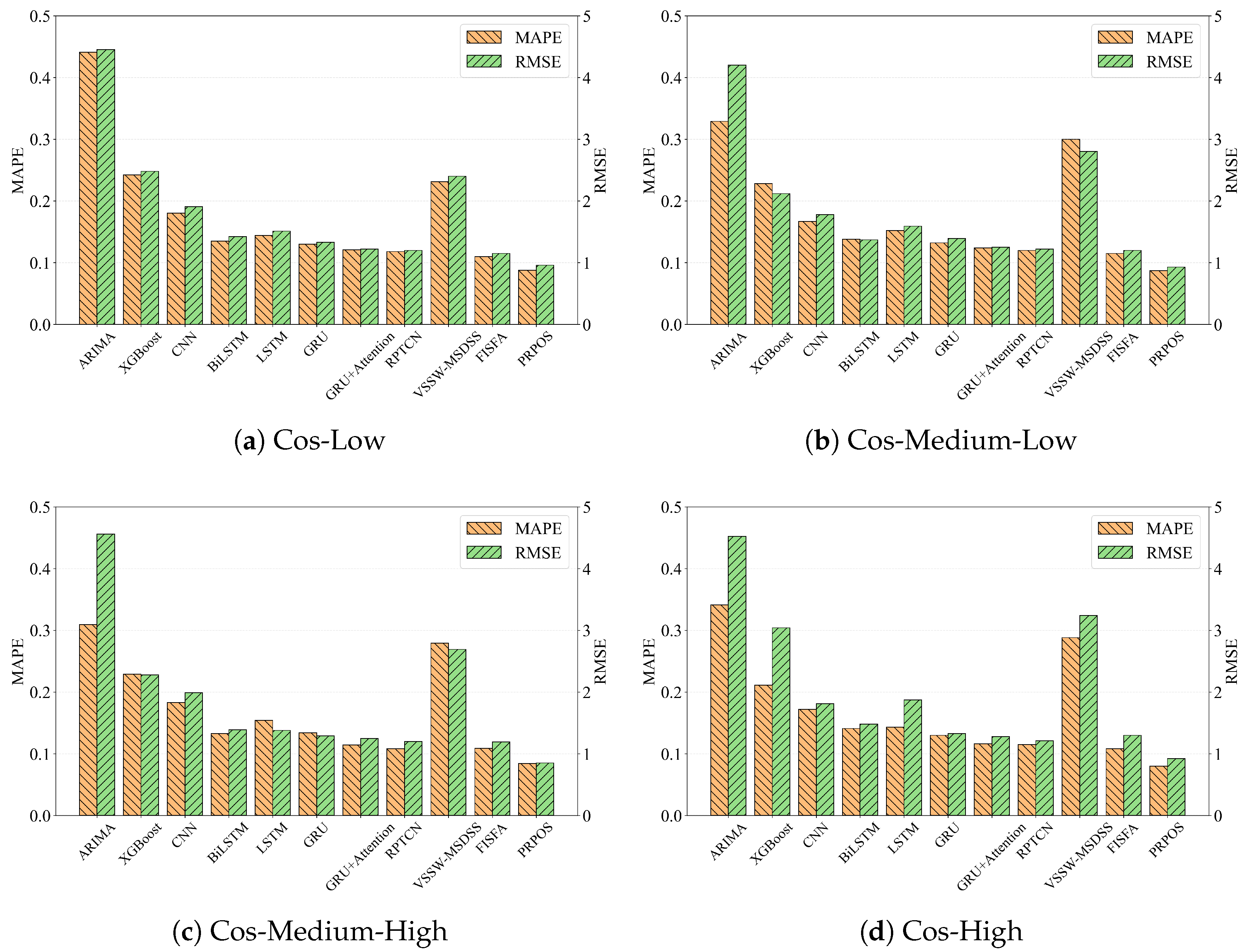
To evaluate the resource prediction performance of PRPOS under diverse utilization patterns, we classified the CPU usage sequences of online services from Alibaba cluster trace v2018 dataset based on their average cosine similarity of periodic patterns obtained through PRPOS’s period detection method. These sequences were grouped into four categories according to similarity ranges—[0.8, 0.85] (Cos-Low), [0.85, 0.9] (Cos-Medium-Low), [0.9, 0.95] (Cos-Medium-High), and [0.95, 1] (Cos-High)—each reflecting a distinct periodic characteristic. From each category, ten sequences were randomly selected for experimentation. To ensure a fair comparison, all baseline methods use the 60 most recent data points as input, matching the total historical data volume of PRPOS, which integrates 10 points from the current cycle and 5 historical cycles (10 points each).

Figure 6 illustrates the overall performance of PRPOS and baseline methods. PRPOS consistently outperforms all baselines across all four test groups, achieving the best results in online service resource prediction. Specifically, it attains an average improvement of 45.3% and a maximum of 80% in MAPE, along with an average improvement of 44.3% and a maximum of 81.4% in RMSE. PRPOS achieves superior performance by explicitly modeling periodicity in resource usage. By intelligently incorporating both short-term dependencies (from the current cycle) and long-term dependencies (from historical cycles), PRPOS effectively captures both immediate variations and recurring patterns. This dual-temporal approach proves more accurate than methods that either ignore periodic features or rely solely on transformer-based dependency modeling.

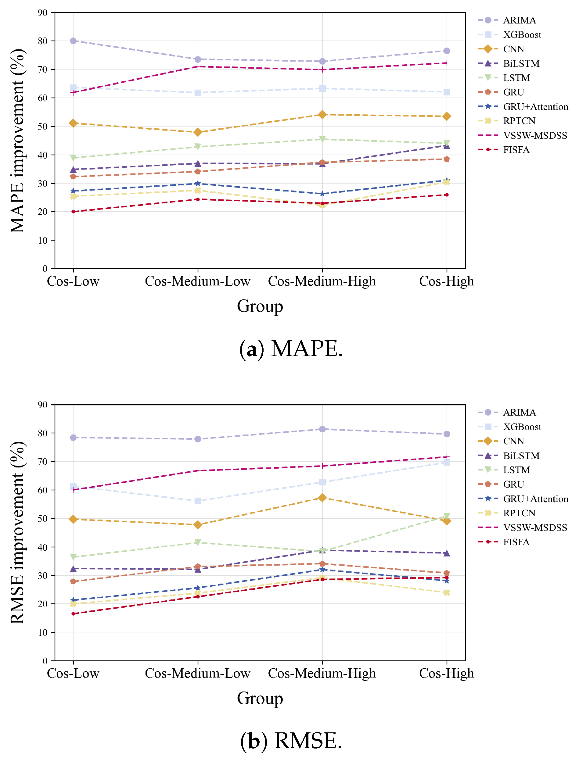
We further observe that the performance improvement of PRPOS becomes more pronounced as the trend similarity across cycles increases. As illustrated in Figure 7, which shows the relative improvement in both MAPE and RMSE over baseline methods, PRPOS achieves significantly greater accuracy gains in groups with higher cosine similarity. For example, compared to the GRU-based model, as similarity increases from [0.8, 0.85] to [0.95, 1], PRPOS attains relative reductions in MAPE ranging from 32.3% to 38.5%, and in RMSE from 27.8% to 30.8%. This trend highlights the advantage of periodic pattern modeling: Higher inter-cycle trend consistency implies more stable and predictable resource usage, thereby improving prediction accuracy.

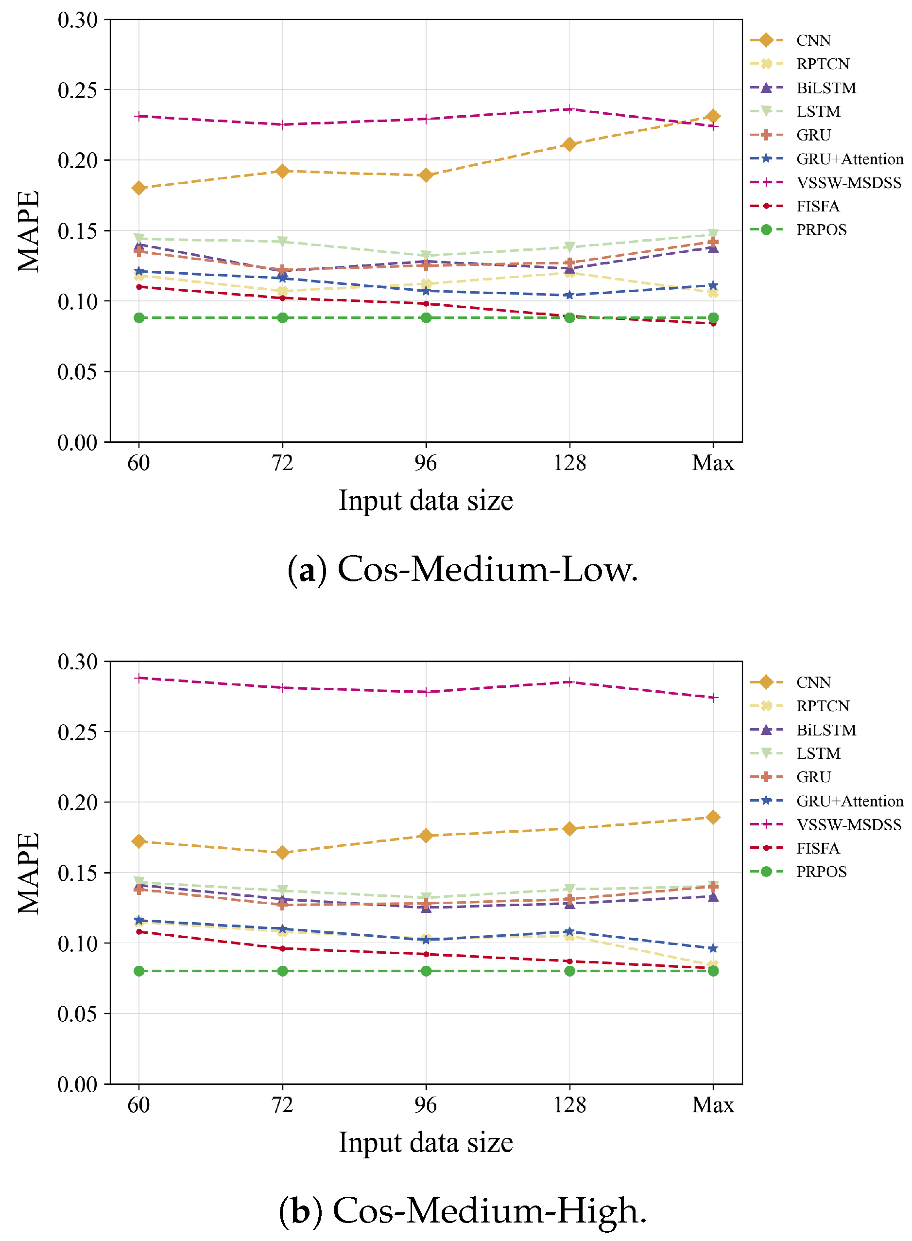
To evaluate the impact of input length on model performance, we maintained PRPOS’s fixed 60-data-point input architecture (comprising the 10 most recent observations plus 5 × 10 phase-aligned historical points) while progressively increasing the sequence lengths of baseline deep learning models to assess their capacity for leveraging extended historical contexts. Specifically, we extended the input length to 72, 96, 128, and maximum feasible lengths (denoted as “$Max$”) for all selected baselines except VSSW-MSDSS. Considering the computational constraint during model training, the maximum lengths were configured as 200 for CNN-based model, 256 for RNN-style models and RPTCN, and 512 for FISFA. We employ the Cos-Medium-Low and Cos-Medium-High service groups for this set of the experiments.

As shown in Figure 8, prediction accuracy does not improve monotonically with longer historical windows. PRPOS consistently outperforms baselines even under the same historical data scale. This is because (1) overly short windows in baseline models fail to capture short-term patterns, while (2) excessively long windows introduce noise and outliers that impair prediction. In contrast, PRPOS maintains robust performance by selectively retaining the most relevant historical data and explicitly modeling inter-cycle trends.

Finally, to validate the robustness of PRPOS, we evaluated its predictive performance on the Cos-Low and Cos-High service groups by varying two key parameters: the sampled window size per cycle and the number of historical cycles used for prediction.

In our experiments, we use the configuration of 10 samples per cycle and 5 historical cycles, which has been employed in our preceding experiments, as the baseline. As illustrated in Figure 9 and Figure 10, the model demonstrates notable robustness. Both MAPE and RMSE remained stable as the sample window size per cycle increased from 8 to 64. A noticeable performance degradation occurred only when the window size was drastically reduced to 4, which resulted in a MAPE increase of up to 20% compared to the baseline. For all other configurations, the deviations in MAPE and RMSE were confined within 3.75% and 2.28%, respectively. Similarly, varying the number of historical cycles from 3 to 7 induced marginal deviations within 7.5% for MAPE and 6.63% for RMSE. However, reducing the cycles to 2 caused a sharp performance decline, increasing MAPE and RMSE by approximately 28.75% and 44.57%, respectively. These results confirm that PRPOS exhibits strong robustness across a wide range of parameter settings, provided they are chosen within appropriate bounds.

Furthermore, compared to the baseline configuration, increasing either parameter did not yield significant performance gains. This suggests that the default setup offers a favorable trade-off between prediction accuracy and computational efficiency.

B.

Period Detection Performance

In this section, we evaluate PRPOS’s novel period detection method, specifically optimized for time series data characterized by consistent temporal trends and heterogeneous magnitude patterns. The experimental dataset and baseline methods are described detail in part A of Section 4.1.

Figure 11 summarizes the accuracy of all methods across different period lengths and under varying degrees of magnitude heterogeneity. PRPOS consistently achieves the highest period detection accuracy in all scenarios. By applying normalized HP filtering and rank-based ACF to mitigate inter-cycle magnitude variations, PRPOS significantly outperforms both SAZED and findFrequency across different period lengths, with an average accuracy improvement of 109.6% and a maximum improvement of 240%.

We further analyze two selected subsets from the 500 synthetic resource usage sequences: a light-variation subset (baseline: 5–10%, fluctuation intensity: 1–10% of the baseline) and a heavy-variation subset (baseline: >10%, fluctuation intensity > 10% of the baseline). Our experimental results demonstrate that PRPOS’s period detection method achieves accuracy improvements of 179.7% on average(up to 304.8%) over SAZED and findFrequency on these subsets. Notably, in experiments with the heavy-variation group compared to the light-variation group, PRPOS achieves higher accuracy improvement, validating the effectiveness of normalization and rank transformation operations.

Among the four baseline methods, RobustPeriod achieves the best detection performance, matching PRPOS in accuracy thanks to its MODWT decomposition, Huber robust estimation, and joint time–frequency validation. However, computational cost comparisons reveal significant differences. As shown in

Table 2. Comparison of computational efficiency for period detection methods.

Methods	Period Size
	[800–1000)	[1000–1200)	[1200–1400)	[1400–1600)	[1600–1820]
PRPOS	0.044	0.082	0.135	0.154	0.206
RobustPeriod	69.485	201.89	409.806	563.839	780.353
SAZEDopt	0.087	0.154	0.224	0.321	0.358
SAZEDmaj	0.043	0.072	0.109	0.157	0.181
findFrequency	0.00046	0.00141	0.00173	0.00250	0.00297

Note: For each group, the lowest computational cost is in bold and the highest is underlined.

, PRPOS maintains sub-second execution times across all period lengths, while RobustPeriod’s runtime grows sharply with longer periods—reaching up to 3788× slower than PRPOS for periods in [1600, 1820]. This efficiency gap stems from their underlying mechanisms: PRPOS leverages low-complexity normalized HP filtering and rank-based ACF, which exploit monotonic cosine similarity to terminate corrections early, whereas RobustPeriod incurs higher overhead from DWT-based frequency decomposition and DFT-based heuristic searches. Notably, findFrequency incurs the lowest computational cost among all methods but suffers from a 2.4-fold reduction in accuracy, attributable to spectral leakage resulting from its simplistic frequency-domain approach.

C.

Ablation Study

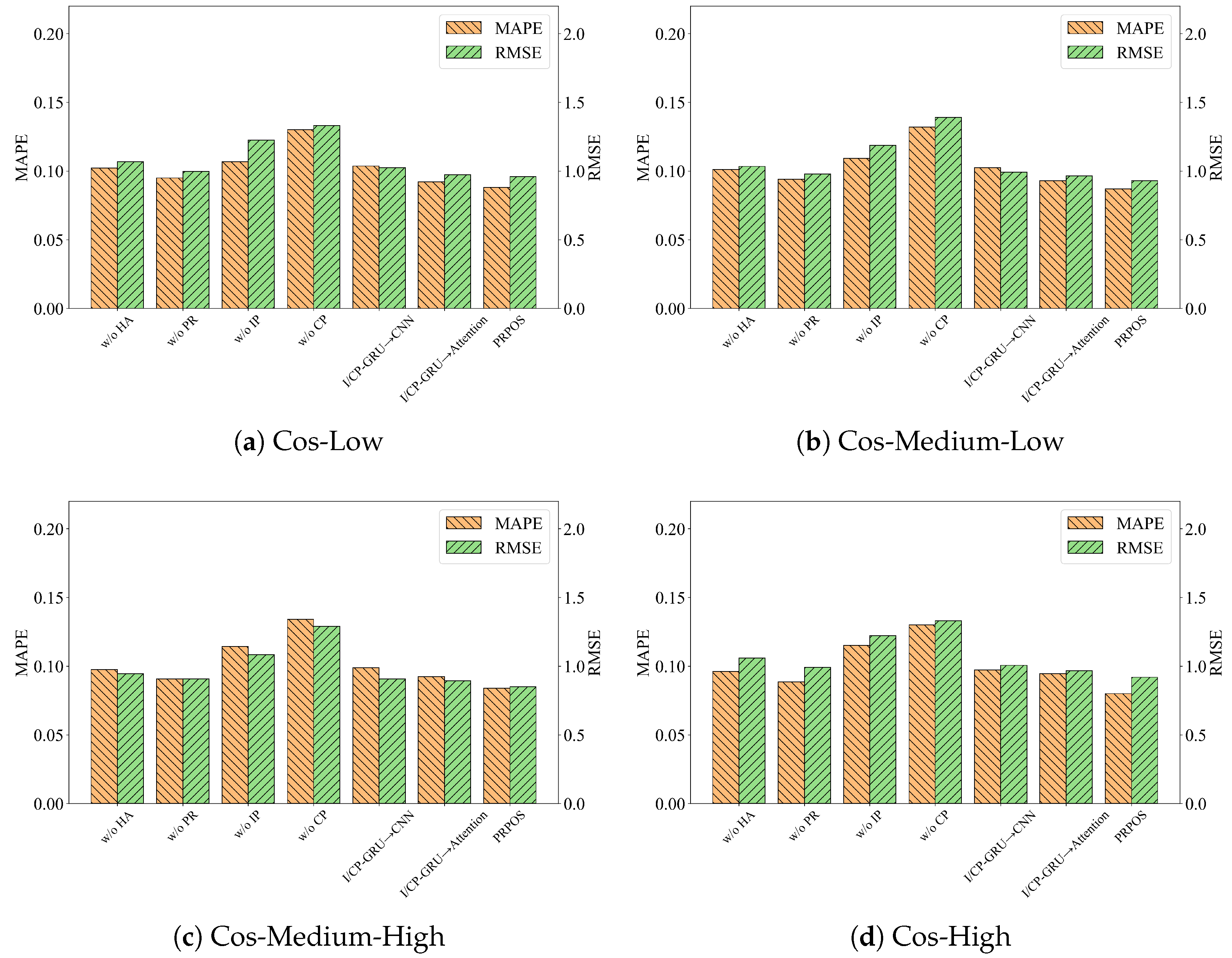
To thoroughly assess the contributions of individual components in the PRPOS prediction model, we perform ablation studies comparing the complete model with its variants, with results detailed in Figure 12. All ablated versions show measurable accuracy degradation compared to the full PRPOS model, which achieves superior performance through its dual capability to perform (1) robust period detection via distribution-resistant normalization and period correction to handle magnitude variations and (2) comprehensive dependency modeling that simultaneously captures both short-term in-period relationships and long-term cross-period patterns across historical sequences.

Effectiveness of the period detection method: We conduct two ablation studies on the three key components in our period detection method. First, replacing normalized HP filtering and rank-based ACF with conventional HP filtering and standard ACF (w/o HA) results in an average increase of 17.17% in MAPE and 12.2% in RMSE across all datasets, confirming the importance of distribution-resistant normalization in reducing period detection noise. Removing the cosine similarity-based refinement component (w/o PR) causes a milder degradation, with MAPE increasing by 8.6% and RMSE by 5.9%, indicating its role in providing additional noise suppression beyond the baseline detector.

Effectiveness of the resource prediction model: To evaluate the effectiveness of our resource prediction model, which consists of in-period and cross-period components, we construct two ablation variants. The w/o IP variant is constructed by removing in-period from the model while retaining cross-period’s structure and inputs; results show that this leads to a 31.7% increase in MAPE and a 28.9% rise in RMSE, underscoring the importance of short-term historical patterns. The w/o CP variant removes the cross-period component and extends in-period’s input to the latest 60-step history; this configuration fails to capture long-term periodic features—even with matched input length—causing a further 55.4% increase in MAPE and a 46.1% rise in RMSE.

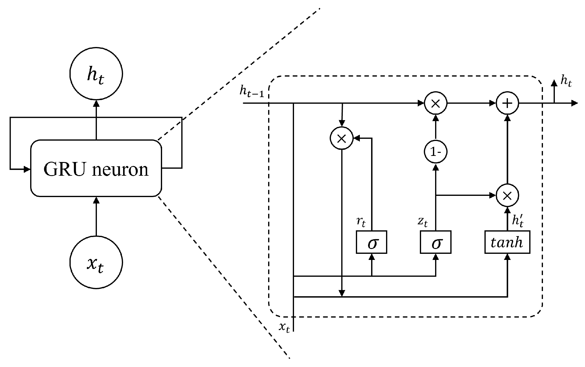
Effectiveness of Sequential Modeling Units: To validate the effectiveness of using GRUs for sequential modeling in both the in-period and cross-period components, we constructed two ablation variants—I/CP-GRU→CNN and I/CP-GRU→Attention—replacing the GRU units with convolution layers and a standard self-attention module (with positional encoding), respectively. Compared to the complete model, the CNN variant shows an average increase of 18.7% in MAPE and 7.3% in RMSE, confirming that GRU outperforms CNN in capturing temporal trends and short-term dependencies. However, replacing GRU with a self-attention mechanism also degrades performance (MAPE: 9.9%, RMSE: 3.8%). This is because our periodicity-based approach splits fixed-length sequences into historical cycles and selects phase-aligned short sub-sequences, negating the self-attention mechanism’s long-sequence weighting. Instead, GRU’s strength in local short-term dependencies prevails. Additionally, GRU’s gating mechanisms adaptively filter noise/outliers for robustness to imperfect data, whereas the attention mechanism is more susceptible to such interference.

5. Discussion

The experimental results in Section 4 affirm the efficacy of PRPOS. This section discusses the core insights behind its success, directly addresses its generalization potential, and outlines its inherent boundaries to guide future works.

5.1. The Value of Explicit Periodicity Modeling

The superior performance of PRPOS stems from its fundamental premise: Periodicity is a primary, structural characteristic of online services that warrants explicit modeling. While deep learning baselines implicitly learn temporal dependencies, their lack of architectural inductive bias for periodicity makes them susceptible to noise and less efficient at leveraging long-range, stable patterns. PRPOS compels the model to distinguish between short-term fluctuations and cyclical trends through its dedicated detection and dual-scale prediction architecture. This approach proves particularly powerful in cloud environments, where identifying the true signal amidst operational noise is crucial for robust predictions.

5.2. Generalization, Boundaries, and Future Paths

Our evaluation focused on CPU utilization because it most saliently exhibits the strong, consistent periodicity that PRPOS is designed to capture. A preliminary analysis of the Alibaba trace revealed that memory and I/O usage for the sampled online services often lacks such clear periodic patterns, instead demonstrating more stochastic and aperiodic characteristics within this dataset. Furthermore, we selected an 8-day evaluation window because it typically encompasses multiple full cycles of the dominant periodicity in online services. This duration thus provides a robust testbed for validating our method’s core principle: the ability to identify and leverage stable periodic patterns.

Consequently, we posit that the framework’s generalization to other resource types depends primarily on the presence of a dominant periodic trend in the target resource. For resources that do exhibit such morphological patterns, our method remains applicable because its detection mechanism is agnostic to absolute values. The current boundaries of PRPOS lie in its single-period architecture and offline detection scheme. Future work will therefore focus on handling multi-periodicity and achieving online adaptation. Developing such an adaptive mechanism is key to addressing longer time series, as it would enable the model to continuously track and adjust to long-term concept drift, where underlying periodicity may gradually evolve.

6. Conclusions

In this paper, we presented PRPOS, a novel periodicity-aware framework for accurate resource prediction in online services. To address the critical yet under-exploited challenge of long-term periodic patterns with consistent trends but significant magnitude variations, PRPOS introduces a two-phase methodology: a robust period detection mechanism combining normalized-weighted HP filtering, rank-based ACF and cosine similarity measurement, followed by a dual-scale GRU predictor that explicitly leverages the detected period to model both in-period and cross-period dependencies.

Extensive evaluations on the Alibaba cluster trace demonstrate that PRPOS achieves an improvement over state-of-the-art baselines, with an average reduction of 45.3% in MAPE and 44.3% in RMSE. These quantitative results solidly validate the efficacy of explicitly integrating periodicity into the resource prediction pipeline.

The practical value of PRPOS lies in its ability to provide cloud operators with more accurate and robust predictions for dynamic resource provisioning. By enabling more informed autoscaling and scheduling decisions, our framework paves the way for enhanced QoS assurance and cost reduction in cloud data centers. In future work, we will extend PRPOS to handle multi-periodic patterns and integrate its predictions into real-world scheduling systems.