Article

A Multi-Objective Artificial Bee Colony Algorithm Incorporating Q-Learning Search for the Flexible Job Shop Scheduling Problems with Multi-Type Automated Guided Vehicles

1
Shenyang Institute of Automation, Chinese Academy of Sciences, 114 Nantajie, Shenyang 110016, China
2
University of Chinese Academy of Sciences, 19 Yuquanlu, Beijing 100049, China
*
Author to whom correspondence should be addressed.
Appl. Sci. 2025, 15(20), 10948; https://doi.org/10.3390/app152010948
Submission received: 11 September 2025 / Revised: 4 October 2025 / Accepted: 6 October 2025 / Published: 12 October 2025

Abstract

The flexible job shop scheduling problem (FJSP) with transportation resources such as automated guided vehicles (AGVs) is prevalent in manufacturing enterprises. Multi-type AGVs are widely adopted to transfer jobs and realize the collaboration of different machines, but are often ignored in current research. Therefore, this paper addresses the FJSP with multi-type AGVs (FJSP-MTA). Considering the difficulties caused by the introduction of transportation and the NP-hard nature, the artificial bee colony (ABC) algorithm is adopted as a fundamental solution approach. Accordingly, a Q-learning hybrid multi-objective ABC (Q-HMOABC) algorithm is proposed to deal with the FJSP-MTA. First, to minimize both the makespan and total energy consumption (TEC), this paper proposes a novel mixed-integer linear programming (MILP) model. In Q-HMOABC, a three-layer encoding strategy based on operation sequence, machine assignment, and AGV dispatching with type selection is used. Moreover, during the employed bee phase, Q-learning is employed to update all individuals; during the onlooker bee phase, variable neighborhood search (VNS) is used to update nondominated solutions; and during the scout bee phase, a restart strategy is adopted. Experimental results demonstrate the effectiveness and superiority of Q-HMOABC.

1. Introduction

Throughout the past several decades, with the development of industrial manufacturing models, particularly the shift towards small-batch and multi-variant production requirements, flexible manufacturing has gradually emerged as a focal point of extensive research in both academic and industrial fields [1]. The flexible job shop scheduling problem (FJSP) is a representative intractable combinatorial optimization NP-hard problem that finds extensive application in real-world production scenarios [2]. In the FJSP system, each job comprises a sequence of operations, and these operations must be processed on distinct machines, requiring machine-to-machine transmission [3,4]. To ensure the efficient completion of such transportation tasks, manufacturing enterprises typically employ automated guided vehicles (AGVs) to realize the automatic transfer of jobs between machines [5]. However, some studies often ignore transportation time or simply fold transportation time into processing time. This oversight compromises practical relevance, as processing and transportation operations are tightly linked: preceding operation’s completion time determines the starting time of the next transportation operation, while transportation time directly determines the subsequent operation’s start time [6,7]. Consequently, integrated scheduling of production and transportation resources is critical for generating actionable and feasible solutions. FJSP with AGV transportation resources (FJSP-T) traditionally addresses three subproblems: operation sequence, machine assignment, and AGV dispatching. While extensive research has addressed the FJSP-T problem, most studies assume a single AGV type and overlook the impact of AGV heterogeneity [8]. For example, different load/empty speeds and energy consumption levels will affect the total energy consumption (TEC) and production cycle. In practical manufacturing environments, however, workshops rarely rely on one single AGV type. Instead, due to budget limitations, space constraints, and diversity of transportation requirements, it is common to deploy a heterogeneous fleet of AGVs with distinct physical and operational characteristics. This heterogeneity may include variations in acceleration profiles, load/empty travel speeds, and energy consumption patterns under different operating states [9]. Such heterogeneity inherently influences both transportation efficiency and the overall energy consumption of the production system. Neglecting these differences not only risks underestimating the actual TEC but also overlooks potential trade-offs between makespan and energy usage [10].
There is currently a lack of research on multi-type AGVs that integrate energy consumption and makespan. To bridge this gap, this paper extends the conventional FJSP-T framework by introducing AGV-type selection as a fourth subproblem alongside operation sequence, machine selection, and AGV assignment, thereby formulating a mathematical model for the FJSP with multi-type AGVs (FJSP-MTA). The proposed mixed-integer linear programming (MILP) model explicitly incorporates AGV heterogeneity into the integrated scheduling process, enabling a coupled optimization of production and transportation resources that more accurately reflects workshop realities. In doing so, our study aims at the simultaneous minimization of makespan and TEC, aligning with both productivity and sustainability imperatives. This dual objective formulation not only enhances the operational feasibility of generated schedules but also provides decision-makers with actionable insights for achieving balanced, energy-efficient, and cost-effective manufacturing operations.
In recent years, learning-based methods that integrated heuristic algorithms with reinforcement learning (RL) have been developed to solve FJSP [11,12,13]. This paper presents a novel multi-objective approach called the Q-learning hybrid multi-objective artificial bee colony algorithm (Q-HMOABC) to solve the FJSP-MTA optimization model, and its inspiration is drawn from reinforcement learning. This paradigm combines the global search capabilities of heuristic algorithms with the self-learning abilities of RL, significantly improving optimization performance and generalization. Pareto-optimal solutions solved by Q-HMOABC have better global convergence, local diversity, and shorter running time. This algorithm has distinct advantages for solving the FJSP-MTA.
The main innovations of this paper are summarized as follows.
(1)
Novel MILP model: A MILP model with the objective of minimizing makespan and TEC is developed to formulate the FJSP-MTA.
(2)
Novel algorithm framework: An efficient Q-HMOABC algorithm is designed to efficiently address the FJSP-MTA, and improved strategies are adopted in three ABC phases. Here, Q-HMOABC is formed by embedding the Q-learning RL method into the employed bee phase of the ABC algorithm.
(3)
Extensive experiments: Unconstrained benchmark functions and benchmark instances are conducted to test the performance of Q-HMOABC, where the statistical results illustrate the superiority of the proposed algorithm in solving the FJSP-MTA.
The remainder of this paper is organized as follows: Section 2 reviews existing studies on the FJSP-T and relevant solving methods. Section 3 describes the problem and proposes a detailed MILP model. Section 4 explains Q-HMOABC from multiple perspectives. Section 5 presents validation experiments in detail. Finally, Section 6 concludes the study and suggests directions for future research.

2. Literature Review

To the best of our knowledge, there is no literature aimed at solving the FJSP-MTA by using Q-HMOABC. Therefore, this paper conducts a review of the relevant literature, including studies on the FJSP-T and existing state-of-the-art work relating to the solving method.

2.1. FJSP with AGV Transportation Resources

The initial work on the FJSP-T was carried out by Raman et al. [14]. A mixed-integer programming model was formulated for the problem, with the objective of minimizing the makespan. In the study, the transportation process was conceptualized as a general operation, a decision that constrained the adaptability of the vehicles. In order to overcome this limitation, a nonlinear mixed-integer programming model was developed and a heuristic algorithm that incorporated a sliding time window was designed to generate a conflict-free schedule [15]. Subsequent to this, the research on the FJSP-T has gradually become more widespread, driven by both theoretical research and industrial technology. Ham et al. introduced two novel constraint programming models by integrating transfer robots in the FJSP [16]. Pan et al. [17] proposed a learning-based multi-population evolutionary optimization (LMEO) and used multiple heuristics for population initialization. Yan et al. [3] developed an FJSP model under finite AGV transportation constraints within a digital twin workshop. An improved genetic algorithm with three-layer redundant encoding and corrective decoding was proposed, achieving efficient integration of feasible schedules into the digital twin and demonstrating strong practical applicability. Meng et al. [18] proposed an improved genetic algorithm (IGA) for solving the multi-AGV flexible job shop scheduling problem, explicitly considering a limited number of AGVs. The IGA includes a population diversity check mechanism that maintains search robustness and, when tested on five benchmark sets, not only outperformed state-of-the-art algorithms but also found new best-known solutions for instances. Han et al. [19] proposed a novel dual-population collaborative genetic algorithm (DCGA) and introduced a new MILP model for small-sized instances, and designed DCGA with two distinct decoding methods and a dual-population framework. Experimental results demonstrated that the approach improved 18 best-known benchmark solutions and achieved optimal results on small-scale cases. Homayouni et al. [20] proposed a late acceptance hill-climbing (LAHC) heuristic, which found high-quality solutions with less computational time. Afterward, Homayouni et al. [21] proposed a multi-start biased random key genetic algorithm (BRKGA) that employs greedy heuristic rules to select machines and AGVs. Liu et al. [22] developed an MILP to simultaneously minimize both makespan and comprehensive energy consumption by modeling time-node dynamics and energy use of machines and AGVs. Zhang et al. [23] proposed energy-efficient flexible workshop scheduling (EFJS-AGV) for multiple autonomous guided vehicles (AGVs) to address the issue that existing research has not yet incorporated green indicators into manufacturing and logistics scheduling frameworks.

2.2. Solving Methods

Many methods have been applied to address the FJSP-T and its extensions, including the exact algorithm (e.g., branch and bound algorithm, CP, and MILP), heuristic, RL, and commercial solver (e.g., CPLEX and Gurobi). Fontes et al. [24] constructed a new MILP model for joint production and transportation scheduling problems. The proposed modeling method utilizes two sets of interrelated chain decisions and is highly efficient in solving the optimal solution of benchmark problem instances using the Gurobi solver. Heuristic algorithms have been developed as the main tools because of their ability to solve large-scale problems efficiently, which exceeds the capabilities of the exact algorithm, including GA (Zhang et al.) [25], PSO (Ren et al.) [26], and ABC (Gao et al.) [27]. RL has made breakthroughs in many fields in recent years. The combination of RL and heuristic methods has become an important research focus in the FJSP-T. Known as learning-based methods, this approach gives heuristic algorithms the ability to learn from experience. With these abilities, the algorithms can adjust their search strategies and choose parameters more effectively, adapting to different scheduling conditions and improving solution quality. Dong et al. [28] formulated the FJSP-T as an MDP and proposed a heuristic-assisted Deep Q-Network (HA-DQN), integrating heuristic rules to reduce action-space complexity. Thid method demonstrates notable gains in both solution quality and computational speed versus traditional heuristics and pure DRL methods. Cheng et al. [29] proposed both exact and approximate methods for the energy-efficient FJSP-T (EFJSP-T). The exact method employed a novel MILP formulation using the epsilon method, and an approximate approach based on multi-population evolution of imitation learning (IL) was introduced to enhance the efficiency of solution space exploration. However, it remains limited to a single type of AGV. LI et al. [30] proposed a hybrid algorithm combining RL and the ABC algorithm for the FJSP with lot streaming, and RL was developed by building mappings between the environment and schemes of sublots. Xu et al. [31] proposed a solution that transforms the FJSP into a Markov Decision Process (MDP) and employs RL techniques for resolution, and designed 16 composite dispatching rules. Similarly, the study also assumed that only one type of AGV exists. Zhang [32] proposed an optimization scheme that minimizes the weighted sum of the makespan and TEC for the distributed FJSP (DFJSP) involving crane transportation. Yang et al. [33] proposed a digital twin–assisted predictive rescheduling method that generates proactive schedules using order-arrival hypotheses.

3. Problem Description and Formulation

In this section, a comprehensive description and analysis of the FJSP-MTA are provided first. Subsequently, the notations and definitions to the problem are listed. Next, a corresponding MILP model is formulated. Finally, an example of an FJSP-MTA is provided to illustrate the MILP model. Analyzing the transportation scenarios of the FJSP-MTA enables a deeper exploration of its domain knowledge, thereby establishing the foundation for subsequent algorithm design.

3.1. Problem Description

The FJSP-MTA is described as follows: a given number of jobs I = {I1, I2, …, In} are processed on a set of machines K = {K1, K2, …, Km}. Each job contains multiple operations Ji = {J1, J2, …, Jni}, which can be processed on multiple processing machines. The transfer between job’s operations is carried out by T = {1, 2, 3, …, t} types of AGV V = {V1, V2, …, VnV}. The job and AGV are initially in the loading and unloading (LU) position, and there is a certain distance between the LU and machines. For each job, when the current operation is performed on a machine, it needs to be transported to the next machine by an AGV for the next operation. The transportation time between two machines and the processing time of each operation on the compatible machine are known in advance. Machines can be categorized into two states: the processing state and the waiting for processing state. Due to the differences in energy consumption, machines consume energy when processing the job and generate idle energy consumption while waiting to process the job. The transportation process of AGVs is also classified into two types: empty travel and load travel. Empty travel represents that the AGV needs to travel from the current machine or LU position to the machine position to pick up the job, while the load travel represents that the AGV takes the job and transports it to the target machine position. The same AGV consumes energy when loading the job and generates empty energy consumption while picking up the job.

Assumptions

The FJSP-MTA satisfies the following assumptions:
  • Initial state constraint: All machines and AGVs are available at time 0, and all jobs can be processed at time 0.
  • Each machine has a buffer zone that can be used to park AGVs and store jobs, and has sufficient buffering capacity.
  • Each machine can process at most one operation at a time.
  • Each AGV can transport at most one job or be empty at a time.
  • The processing task of jobs cannot be interrupted as soon as it starts.
  • The transportation task of jobs cannot be interrupted as soon as it starts.
  • The loading and unloading time are excluded in the transportation time.
  • The job does not return to the LU area once it has been completed.
  • Machine and AGV breakdown during operation are not considered, with sufficient AGV battery power.
  • The last operation of each job does not need to be transported after it is finished.

3.2. Formulation of MILP Model

In the FJSP-MTA, we need to deal with the FJSP and the AGV dispatching problem simultaneously. It can be divided into four subproblems: (1) machine assignment problem, deciding the processing machine for each job; (2) machine scheduling problem, defining the processing sequence of the jobs on each machine; (3) AGV assignment problem, determining which type of each AGV to assign; and (4) AGV scheduling problem, resolving the allocation of the transportation resources for each job.
The objective function of the FJSP-MTA is to simultaneously minimize the makespan Cmax and TEC. The FJSP-MTA is formulated in this paper as a MILP model, using the notations in Notations.
M i n i m i z e : F ( x ) = T E C + C max
where Cmax is the completion time of the last operation Oi,j of last processing job I. TEC can be divided into three components: machine processing energy consumption (MPEC), machine idle energy consumption (MIEC), and AGV transportation energy consumption (ATEC). They are calculated as shown in the following Equation (2):
T E C = M P E C + M I E C + A T E C
The formulas for the three terms are as follows:
M P E C = i = 1 n j = 1 n i k k ( i , j ) t = 1 T v = 1 n V P P k P T i , j , k X i , j , k , t , v
M I E C = k k ( i , j ) I P k E M k i = 1 n j = 1 n i t = 1 T v = 1 n V P T i , j , k X i , j , k , t , v
A T E C = i = 1 n j = 1 n i v = 1 n V v = 1 n V k k ( i , j ) k k ( i , j ) t = 1 T X i , j 1 , k , t , v X i , j , k , t , v T T k , k , t A P l o a d t A P e m p t y t + t = 1 T v = 1 n V E A t , v A P e m p t y t
The first term of ATEC’s calculation is load energy consumption, and the second term is empty energy consumption.
The MILP model is subjected to constraint sets (3)–(17).
S i , j + P T i , j , k E M k + M 1 t = 1 T v = 1 n V X i , j , k , t , v             i I , j J i , k k ( i , j )
S i , j + k k ( i , j ) T T k , k , t + P T i , j , k t = 1 T v = 1 n V S A i , j + 1 , t , v + M 1 t = 1 T v = 1 n V S A i , j + 1 , t , v i I , j 1 , 2 , , n i 1 , k k ( i , j + 1 )
S i , j + t = 1 T v = 1 n V X i , j , k , t , v P T i , j , k S i , j + M 3 Y M i , j , i , j t = 1 T v = 1 n V X i , j , k , t , v t = 1 T v = 1 n V X i , j , k , t , v i I , i I , i < i , j J i , j J i , k k ( i , j ) k ( i , j )
S i , j + t = 1 T v = 1 n V X i , j , k , t , v P T i , j , k S i , j + M 2 + Y M i , j , i , j t = 1 T v = 1 n V X i , j , k , t , v t = 1 T v = 1 n V X i , j , k , t , v i I , i I , i < i , j J i , j J i , k k ( i , j ) k ( i , j )
1 M 2 t = 1 T v = 1 n V X i , j , k , t , v t = 1 T v = 1 n V X i , j + 1 , k , t , v t = 1 T v = 1 n V X i , j + 1 , k , t , v i I , j { 1 , 2 , , n i 1 } , j J i , k k ( i , j ) , k k ( i , j + 1 )
Y T t , v , i , j , i , j + Y T t , v , i , j , i , j = 1             i , i I , j J i , j J i , O i , j O i , j , t T , v n V
S i , n i + k k ( i , n i ) t = 1 T v = 1 n V P T i , n i , k X i , n i , k , t , v C m a x             i I
k k i , 1 X i , 1 , k , t , v T T 0 , k , t S A i , 1 , t , v             i I
S A i , j , t , v E A t , v             i I , j J i , t T , v n V
S i , j 0             i I , j J i
S i , j t = 1 T v = 1 n V S A i , j , t , v             i I , j J i
E M k 0             k = 1 , 2 , , m
E A t , v 0             t T , v n V
S A i , j , t , v 0             i I , j J i , t T , v n V
t = 1 T v = 1 n V k k i , 1 X i , 1 , k , t , v = 1             i I
where constraint (3) represents the machine shutdown time constraint: the operation must be completed before the machine is shut down. Constraint (4) represents the constraints between process start time and arriving time: the arriving time for each process must precede or be equal to its process start time. Dual constraints (5) and (6) ensure the non-overlapping of the operations arranged on the same machine. Constraint (7) represents adjacent sequential operations constraint: Oi,j and Oi,j+1 are not processed on the same machine. Constraint (8) ensures the non-overlapping transportation of the operations assigned to the same AGV. Constraint (9) represents the makespan constraint: makespan must not be less than the start time of each job plus its subsequent processing time. Constraint (10) limits the transportation of the first operation of each job. Constraint (11) represents the AGV working time constraint: The end time for the same AGV’s transport must precede the arrival of the transport process. Constraint (12) limits the range of decision variable Si,j. Constraint (13) represents the relationship of SAi,j,t,v and Si,j: The start time for operation Oi,j must not precede the arrival time. Constraints (14)–(16) limit the ranges of decision variables EMk, EAt,v, and SAi,j,t,v. Constraint (17) represents that an operation can be assigned on exactly one machine and one AGV.

3.3. Example of FJSP-MTA

To better comprehend the above-described MILP model for the FJSP-MTA, Figure 1 illustrates a Gantt chart of a feasible schedule with three jobs, three machines, and two types of AGV, one of each type. Table 1 lists the compatible machines and processing time of each operation Oi,j. Table 2 shows the transfer time between machines for the two types of AGV. M0 represents loading/unloading point.
The parameters in the MILP model describe the above Gantt chart as follows: energy consumption parameters of three machines include PP1 = 2.5, PP2 = 2.1, PP3 = 2.7, IP1 = 1.5, IP2 = 1.2, and IP3 = 1.6. Energy consumption parameters of two types of AGVs include A P l o a d 1  = 2.4, A P l o a d 2 = 1.2, A P e m p t y 1 = 1.6, and A P e m p t y 2 = 0.8. Decision variables include X1,1,1,1,1 = 1, X1,2,2,1,1 = 1, X2,1,3,2,1 = 1, X2,2,2,1,1 = 1, X3,1,2,1,1 = 1, X3,2,1,2,1 = 1; YT1,1,3,1,1,2 = 1, YT1,1,1,2,2,2 = 1, YT1,1,3,1,1,2 = 1, YM1,1,3,2 = 1, YM3,1,1,2 = 1, and YM1,2,2,2 = 1. Start time for each operation include S1,1 = 20, S1,2 = 120, S2,1 = 80, S2,2 = 160, S3,1 = 70, and S3,2 = 160. Shutdown time for three machines include EM1 = 203, EM2 = 215, and EM3 = 130. Arrival time of each vehicle transport job include SA1,1,1,1 = 20, SA1,2,1,1 = 120, SA2,1,2,1 = 80, SA2,2,1,1 = 20, SA3,1,1,1 = 70, and SA3,2,2,1 = 160. End transporting time of two AGVs include EA1,1 = 150 and EA2,1 = 160. The machine processing energy consumption is MPEC = 672; the machine idle energy consumption is MIEC = 135. Only the machine M1 generated idle energy consumption after startup. The AGV total energy consumption is ATEC = 488. The total energy consumption generated by the entire workshop is TEC = 1295. All oprerations’ finish time is makespan = 215.

4. Q-Hybrid Multi Objective Artificial Bee Colony (Q-HMOABC)

Due to the NP-hard nature, the ABC algorithm is considered more efficient than exact algorithms for solving the FJSP-MTA on a large scale. However, since the problem involves strong coupling among machine scheduling, transportation assignment, and energy consumption optimization, it is difficult for the standard ABC to obtain high-quality solutions without further enhancement strategies. Recently, the integration of RL into swarm intelligence algorithms has emerged as an effective approach for scheduling optimization. By embedding learning mechanisms such as Q-learning into the search process, the algorithm can adaptively exploit historical experience to guide bees to make decisions and adjust the search direction dynamically. To further balance exploration and exploitation, an improved ABC-based RL algorithm called Q-HMOABC is presented in this work. Moreover, the new population initialization, specific evolutionary phase search method, and strategies for updating populations are introduced to improve and balance the exploration and exploitation.

4.1. Framework of the Q-HMOABC

The framework of the proposed Q-HMOABC consists of four key components. First, a chaotic population initialization method is employed to enhance population diversity at the early stage. Next, a fast nondominated sorting procedure is applied to rank the entire population and provide a structured basis for the subsequent evolutionary process. Then, in the following three phases of the ABC, different strategies are incorporated: during the employed bee phase, a Q-learning mechanism is used to guide the update of all individuals; in the onlooker bee phase, a variable neighborhood search (VNS) is applied to refine nondominated solutions; and in the scout bee phase, a restart strategy is introduced, where individuals that do not improve for a certain number of generations are replaced by randomly generated ones. These components form the integrated framework of Q-HMOABC, aiming to balance exploration and exploitation while maintaining population diversity throughout the search process. The Q-HMOABC framework pseudocode is shown in Algorithm 1.
Algorithm 1: Q-HMOABC
Input: Job and AGV time, energy parameters, population size, learning rate,
    discount factor, exploring rate, restarting number, number of VNS;
Output: OS, MA, AD, Makespan, TEC;
1 Initialize population P 0 = { x 1 , x 2 , , x N } by Tent chaotic map;
2 Define fitness function F ( x ) = C max ( x ) , T E C ( x ) ;
3 Define Q-learning tuple ( S , A , R , Q ) with state s S , operator a A ,
   reward R = ( s , a ) , Q-value Q ( s , a ) ;
4  t 0 ;
5 while t < MaxIter do
6  Perform fast non-dominated sorting on Pt, obtain fronts F1, …, Fk;
7  for each employed bee i { 1 , , N e }  do
8   Select operator a = arg max a Q ( s , a ) with probability 1 ε , else random a;
9   Generate candidate x N a ( x i ) ;
10    Evaluate F ( x ) = ( C max ( x ) , T E C ( x ) ) ;
11    if  F ( x ) F ( x ) then
12     x i x ;
13    Update Q ( s , a ) Q ( s , a ) + α R ( s , a ) + γ max a Q ( s , a ) Q ( s , a ) ;
14for each onlooker bee j { 1 , , N 0 }  do
15    Select xk with probability p k = F x k l N F x l ;
16    Apply x V N S x k ;
17    if  F ( x ) F ( x )  then
18    Update x k x ;
19for each scout bee l { 1 , , N s }  do
20    if no improvement for LN iterations then
21    Restart strategy x l U T , E ;
22 Update Pareto archive A * A * P t
23if stopping criterion satisfied then
24    return non-dominated set  A * ;
25 t t + 1 ;
26 end while

4.2. Solution Representation

The encoding method directly affects the solution space and efficiency of Q-HMOABC. A three-layer coding method based on operation is used to encode a solution in Q-HMOABC. First, the operation sequence (OS) vector is generated, and machine assignment (MA) and AGV dispatching (AD) vector are then determined according to the OS and corresponding constraints. Finally, OS, MA, and AD are combined to represent a solution to the problem. These parameters are described as follows.
OS: The internal number of the OS chromosome gene indicates the serial number of the job, and the sequence of the same number indicates the operation number of the job. For example, as shown in Figure 2a, the first number 3 in OS vector represents the operation O3,1, the number 3 at the sixth position denotes O3,2, and the last position 3 represents O3,3. The priority of operation within the same job is ensured by this code, as O3,1 → O3,2 → O3,3. The length of the vector is equal to the total number of operations.
MA: The location of the element in the candidate machines set is applied to denote the MA vector. The number k in the MA vector denotes that the kth machine in the candidate set is assigned to the operation Oi,j. As shown in Figure 2b, the first number 2 in MA vector indicates that the second machine M3 in the set {M1, M3} is selected, and the third number 3 in MA vector indicates that the third machine M4 in the set {M2, M3, M4} is selected. The machine assignment and processing sequence on every machine are jointly determined by decoding OS and MA vectors based on the given set of candidate machines.
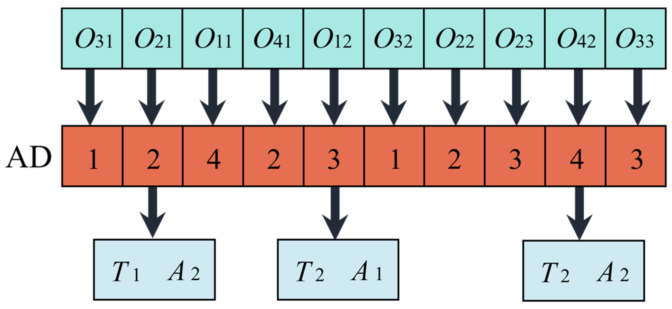
AD: The internal number of the AGV chromosome gene represents the specific vehicle assigned for transportation. In this encoding, different integers are used to distinguish both the vehicle type and its index within the type. For example, numbers 1 and 2 denote the first and second AGVs of type 1, respectively, while numbers 3 and 4 correspond to the first and second AGVs of type 2. For example, as shown in Figure 3, the first number 2 in the AD vector indicates that O2,1 is transported by AGV no. 2 of type 1, the number 3 at the fifth position denotes that O1,2 is transported by AGV no. 1 of type 2, and the ninth position 4 represents O4,2 being transported by AGV no. 2 of type 2. Each gene in the AD vector determines which AGV is responsible for the corresponding transportation task. The length of the AD vector is equal to the total number of transportation tasks in the scheduling problem.

Crossover and Mutation

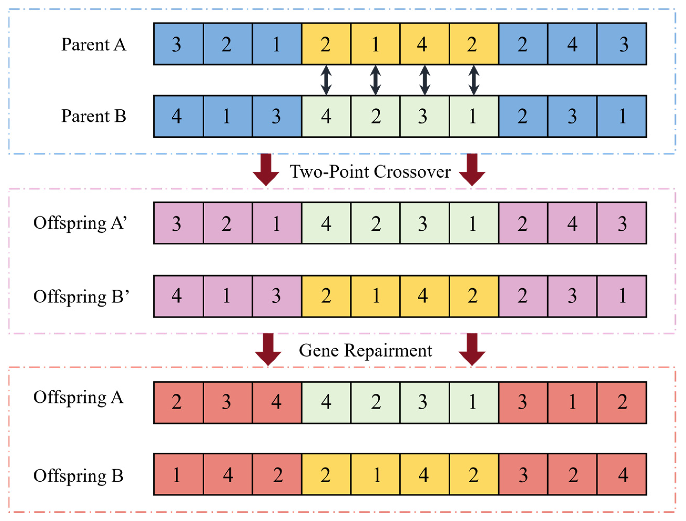
Crossover operations generate new individuals by recombining genes from two parent chromosomes, thereby increasing population diversity. Based on the characteristics of the FJSP-MTA, the encoding methods, and problem constraints of the operation, machine, and AGV gene segments, this work designs different crossover methods to generate new individuals: Specifically, ensure that the number of operations for each job remains unchanged in the offspring after crossover. This paper uses the Partial-Mapped Crossover (PMX) principle to perform crossover operations on OS genes, as shown in the example in Figure 4. Two-point crossover (TPX) is performed first. Select genes from the fourth to the seventh position and swap the middle segments between Parent A and B to generate Offspring A′ and B′. Subsequently, gene repair is performed through process precedence mapping to prevent generating infeasible solutions that violate the precedence relationship among operations within one job. The specific steps involve establishing a mapping relationship for the unswapped genes in Offspring A′ and B′, 1 → 4, 2 → 3, 4 → 1, 3 → 2, thereby generating Offspring A and B. The machine layer also uses TPX. To guarantee that the new machine number is derived from the set of available machines of the original operation, gene repairment is also performed on MA genes.
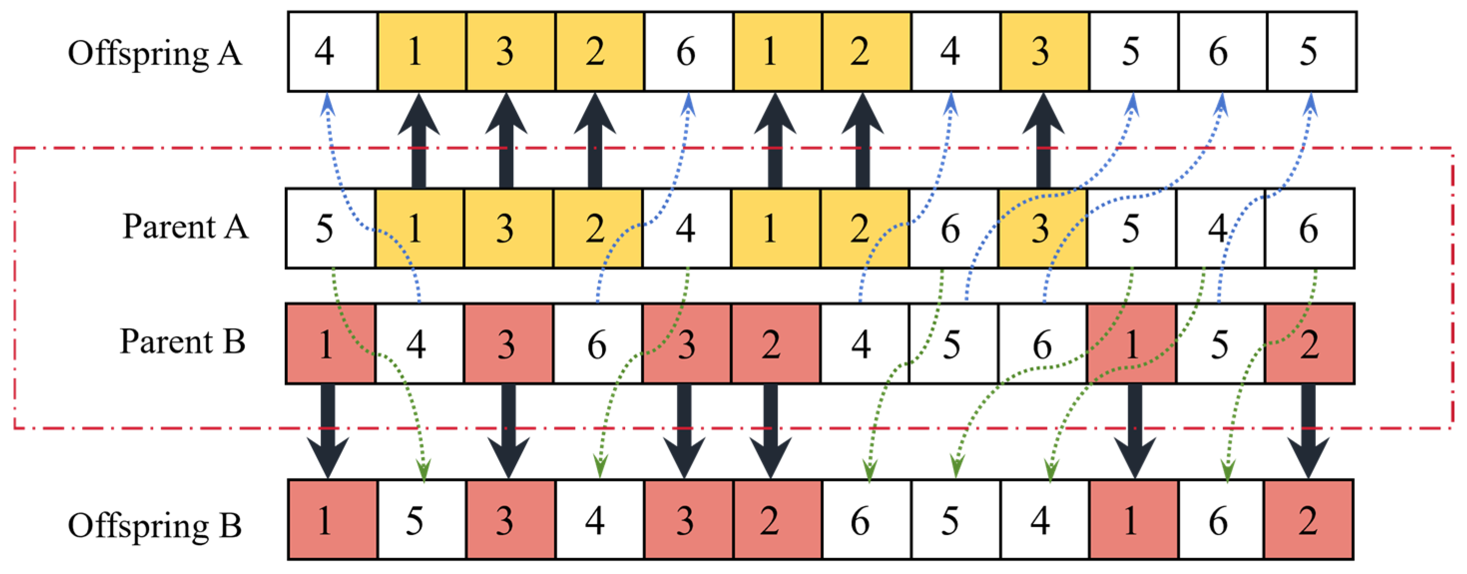
The AGV layer uses position-based crossover (POX), specifically tailored to AGV type and indices. Specifically, the POX operator ensures that each transportation task in the offspring is assigned to a valid AGV while preserving the intended AGV type and its corresponding index. An illustrative example in Figure 5 shows how partial positions are copied from one parent and the rest are sequentially completed from the other, thereby maintaining type-consistent, index-explicit AGV assignments for all transportation tasks. First, randomly generate two parent genes Parent A and B. Copy the genes at positions 2, 3, 4, 6, 7, and 9 from Parent 1 to Offspring A while retaining their original positions. Copy the genes from the remaining positions of Parent B sequentially to the remaining positions in Offspring A. Offspring B undergoes the same process. If a copied gene violates a feasible type restriction, a minimal repair is applied by remapping the gene to another vehicle within the same type, leaving all other positions unchanged.
After crossover, three complementary mutation strategies are applied to sustain diversity and promote local refinement. (i) OS layer: Two methods are used. A two-point swap that exchanges the genes at two uniformly selected positions, and an inversion that reverses the contiguous subsequence between two random cut points. (ii) MA layer: Two methods are used. Swap one machine at a random location; for each selected operation, the machine k is selected from its feasible set k(i,j); Swap three machines k = {1, 2, 3} at random locations: for three selected operations, the machines are selected from their corresponding feasible set k(i,j). (iii) AD layer: The same two mutation strategies as at the MA level are employed.

4.3. Population Initialization

Population initialization critically shapes swarm search: a well-distributed seed set broadens exploration and delays premature convergence, whereas uneven or biased seeding narrows the search and degrades solution quality. Common schemes are concise but limited—random seeding is easy yet often clustered; heuristic seeding injects problem knowledge at the risk of bias and reduced generality. In the FJSP-MTA, where machine assignments and AGV dispatching are tightly coupled and the search space is large and multimodal, these limitations can quickly propagate into an inferior Pareto front.
Therefore, this work adopts chaotic initialization based on the tent map within Q-HMOABC. The tent map produces deterministic, pseudo-random sequences with near-uniform density, ergodicity, and sensitivity to initial conditions. This seeding increases early diversity, improves space coverage, and lowers the risk of local entrapment, while preserving sufficient randomness to sustain exploration as learning and local search proceed. Empirically, it accelerates convergence and yields stronger Pareto approximations, such as higher hypervolume (HV) and lower inverted generation distance (IGD). The tent map used for initialization is formally defined in Equation (18), and it serves as the default population generator in our framework. Where x t p and x t + 1 p denote the current state of the sequence at iteration t and the next state of the sequence at iteration t + 1, p denotes the population size, and a denotes the control parameter.
x t + 1 p = x t p a , 0 < x t p < a , 1 x t p 1 a , a x t p < 1 ,   a ( 0 , 1 )
where the symmetric form is recovered with a = 1 2 , shown in Equation (19):
x t + 1 p = 2 x t p , 0 < x t p < 1 2 , 2 1 x t p , 1 2 x t p < 1 .
We choose an initial value x 0 ( 0 , 1 ) to avoid a dyadic rational, iterate the map for a burn-in period B to eliminate transient effects, and then collect the subsequent chaotic values {u1, u2, u3, …, uN}. Subsequently, by mapping this sequence to each decision variable in the population, such as operation sequence OS, machine assignment MA, and AGV dispatching AD, an initial population of size P can be generated.

4.4. Fast Nondominated Sorting Procedure

The purpose of this procedure is to sort the population based on dominance relationship between solutions. Each solution is compared with every other solution in the population to find which one is a nondominated solution. In our bi-objective FJSP-MTA formulation, we minimize the Cmax and TEC. Fast nondominated sorting classifies a population P = {x1, x2, x3, …, xN} into the Pareto front by the dominance relation of minimization. For any solution p , q P , p dominates q as shown in Equation (20).
p q C max ( p ) C max ( q ) TEC ( p ) TEC ( q ) C max ( p ) < C max ( q )     TEC ( p ) < TEC ( q )
For each pP, define the dominated set and domination count in Equation (21).
S ( p ) = q P | p q   ,   n ( p ) = q P | p q
The first front is F1 = {pP|n(p) = 0}; subsequent fronts are obtained by iteratively “peeling” Fk: for all pFk and qS(p) set n(q) ← n(q) − 1, and then Equation (22) is generated. This yields a partition P = k = 1 K F k with a nondomination rank r x = k x F k . In practice, the front ranks F k guide survivor selection.
F k + 1 = q P   \   i = 1 k F i | n q = 0

4.5. Employed Bee Phase

RL is an adaptive optimization control algorithm that obtains reward through interaction between an agent and its environment, thereby forming a learning strategy. Six basic elements are involved during learning, including the agent, environment, state, action, strategy, and reward, with the learning mechanism as in Figure 6. The agent takes action based on the current state. As the most classic RL algorithm, Q-learning records the agent’s learning experience through a Q-table. The number of rows in the Q-table corresponds to the number of state types, and the number of columns corresponds to the number of actions. The Q-value reflects the rationality of selecting a certain action in each state, with initial Q-values all set to 0. Currently, the Q-learning algorithm is widely applied in hybrid meta-heuristic algorithms, such as using ABC to dynamically adjust parameters, select search operators, and determine algorithm structures. Q-table is used to record the Q-values under the state S t and the corresponding action a t , which indicates the learning experience of the agent, shown in Equation (23). This paper employs the Q-learning algorithm to dynamically select the search strategy for the employed bee phase. The agent selects action based on the ε−greedy strategy, and the update formula for the Q-table is as shown in Equation (24).
s 1 s 2 s t Q s 1 , a 1 Q s 1 , a 2 Q s 1 , a t Q s 2 , a 1 Q s 2 , a 2 Q s 2 , a t Q s t , a 1 Q s t , a 2 Q s t , a t
Q S t , a t = Q S t , a t + α r t + 1 + γ max Q S t + 1 , : Q S t , a t
where a t is the learning rate, γ is the discount factor, r t + 1 is the reward value obtained by taking action a t and interacting with the environment in state S t , and max Q S t + 1 , : represents the maximum value in table Q in state S t + 1 based on the ε -greedy strategy.
In this paper, Q-learning is used to determine the search strategy for employed bees. The pseudocode for employed bee phase is shown in Algorithm 2. The prerequisite for applying the Q-learning algorithm is a reasonable design and division of states and the definition of actions that meet the requirements. In addition, it is necessary to reasonably design the reward function. Employed bee plays a leading role in the ABC algorithm. In the original ABC algorithm, the employed bee searches within a specified area to generate new solutions.
Algorithm 2: Employed Bee Phase with Q-learing
Input: Non-dominated archive Ω, Q-table Q, number of neighbourhood search LS,
    Learning rate, discount factor, exploration rate;
Output: Updated archive Ω;
1 Let current solution be S (the employed bee’s incumbent);
2 Set iteration counter t 1 ;
3 while  t L S  do
4  Observe state s t ϕ ( S ) ;
5  Draw u U ( 0 , 1 ) ;
6  if  u ε  then
7     a t arg max b Q ( s t , b ) ;
8  else
9    Sample a t uniformly from action set;
10  Generate neighbor S * N a t ( S ) ;
11  Evaluate F ( S ) = C max ( S ) , T E C ( S ) and F ( S * ) = C max ( S * ) , T E C ( S * ) ;
12  if   F ( S * ) F ( S )  then
13    S S * ; R t 10 ; Ω UpdateArchive ( Ω , S ) ;
14  else if  F ( S ) F ( S * )
15    R t 0 ;
16  else
17    R t 5 ; Ω UpdateArchive ( Ω , S * ) ;
18  end if
19  Observe s t + 1 ϕ ( S ) ;
20   Q ( s t , a t ) ( 1 r ) Q ( s t , a t ) + r R t + a max b Q ( s t + 1 , b ;
21   t t + 1 ;
22 end while

4.5.1. The State Set

The state can be regarded as the agent’s understanding and encoding for the environment. It typically contains some information about the effects on the environment resulting from decisions taken by the agent. The set of states is composed of all possible states for the problem. Under certain conditions, the agent selects the parameter, and we can obtain the Pareto front after iteration. The change in the Pareto front’s convergence and diversity reflects whether this time parameter selection is meaningful. To represent the agent’s state, two metrics, Ct and Dt, are applied to measure the convergence and diversity of Pareto front Equations (25) and (26):
C t = G D ( P t , P * ) = y P t min x P * x y 2 2 P t
D t = i = 1 N 1 d i d m N 1 d m
where Pt is the Pareto front calculated by the algorithm in each generation, and P is the reference point. The smaller the Ct, the better the convergence, and ΔCt < 0. In Dt, di is the Euclidean distance between adjacent solutions after ordering Pt along one objective, and dm is the mean value of d. The bigger Dt the better diversity, and ΔDt > 0. The steps for selecting the state and action are as follows. State1: ΔCt > 0 and ΔDt > 0; State2: ΔCt > 0 and ΔDt ≤ 0; State3: ΔCt ≤ 0 and ΔDt > 0; and State4: ΔCt ≤ 0 and ΔDt ≤ 0. State1 and State2 occur during the early evolution period. State3 and State4 will happen when the population has converged. These four conditions are regarded as four states of the agent.

4.5.2. The Select Strategy

The strategy is the basis for the agent acting as a given, which determines the exploration and exploitation capabilities of the agent. In the work, the ε−greedy select strategy is applied in Q-HMOABC and expressed as in Equation (27):
ε greedy s = arg   max a   Q S t , a t , ε r Randomly   a A ,     ε < r
where ε is the exploration rate, r is a random number within (0, 1), and max   Q ( S t , a t ) represents the highest expected Q-value at the state S t when the action a is performed. Equation (25) denotes that the agent can adopt action a with probability ( 1 ε ) or a random action with a smaller probability ε ; that is, the agent exploits the learning experience with probability ( 1 ε ) and explores new knowledge at each selection.

4.5.3. The Action Set

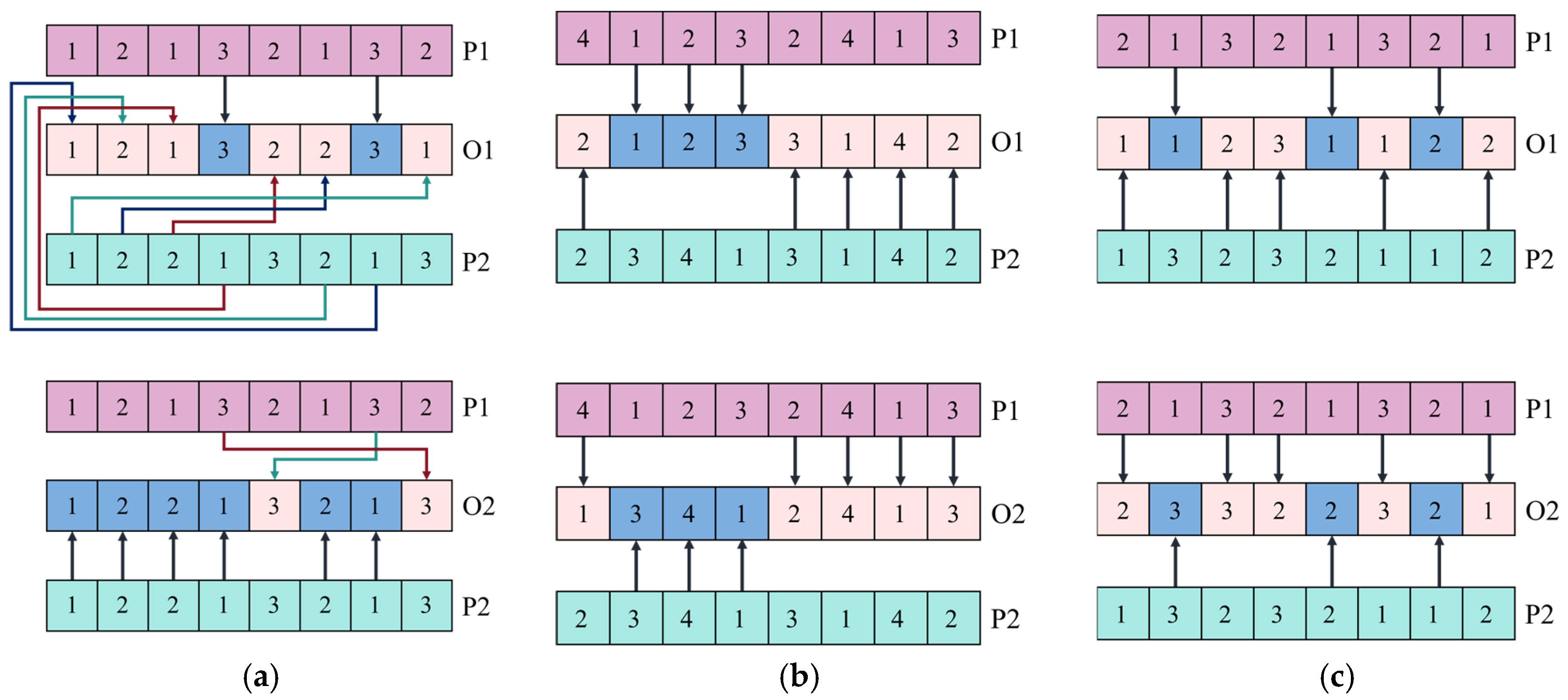
The agent influences its environment by performing the action in RL, and the action set consists of all the actions that the agent can take. The action set consists of eight mutation operators. The four operators for OS are as follows: (1) POX partitions jobs into two subsets and swaps the corresponding subsequences between parents through order-preserving repair; (2) inversion-based POX (IPOX) crossover interleaves job-subset segments from the two parents in their original relative order; (3) inversion mutation selects a contiguous subsequence and reverses it; and (4) insertion mutation removes one operation and reinserts it at another position. The two mutation operators for MA are as follows: (1) single-point mutation reassigns the machine of one selected operation from its feasible set k(i,j); and (2) TPX applies the same reassignment to k randomly chosen operations. The two mutation operators for AD are as follows: (1) single-point mutation reselects the vehicle/type for one operation from its feasible AGV set; and (2) multi-point mutation reselects the vehicle/type for one operation from their feasible AGV set. Some operators are described as follows:
IPOX: This search operator is applied to the OS vector, and its example is shown in Figure 7a for better clarity. The steps are as follows: First, divide the jobs into two subsets, Js1 = {3} and Js2 = {1, 2}. Next, copy from P1 the elements whose jobs belong to Js1 into the same positions of O1, while copying from P2 the elements whose jobs belong to Js2 into the same positions of O2. Finally, for O1, collect from P2 the remaining elements whose jobs are not in Js1, invert their relative order, and sequentially fill the empty positions; for O2, collect from P1 the remaining elements whose jobs are not in Js2, invert their order, and fill the empty positions.
TPX: This search operator is applied to the MA vector. To illustrate TPX more intuitively, an example is provided in Figure 7b. The steps are as follows: First, select two different points a and b in the MS vector. Next, copy the segment P1 [2: 4] to O1 [2: 4] and P2 [2: 4] to O2 [2: 4]. Finally fill the remaining empty positions of O1 sequentially with the elements of P2 outside [2: 4]; and fill the remaining positions of O2 with the elements of P1 outside [2: 4].
MPX: This search operator is applied to the AD vector. An example of MPX is provided in Figure 7c. The processing steps are as follows: First, randomly select three positions in the VD vector. Next, place the elements of P1 at those three positions into the corresponding positions of O1, and place the elements of P2 at the same positions into O2. Finally, fill the empty positions of O1 in order with the remaining elements from P2, and fill the empty positions of O2 with the remaining elements from P1.

4.5.4. The Reward Set

After executing an action, the agent will get a reward. If State1 occurs, Rt = 10; if State2 and State3 occur, Rt = 5; and if State4 occurs, Rt = 0.

4.6. Onlooker Bee Phase

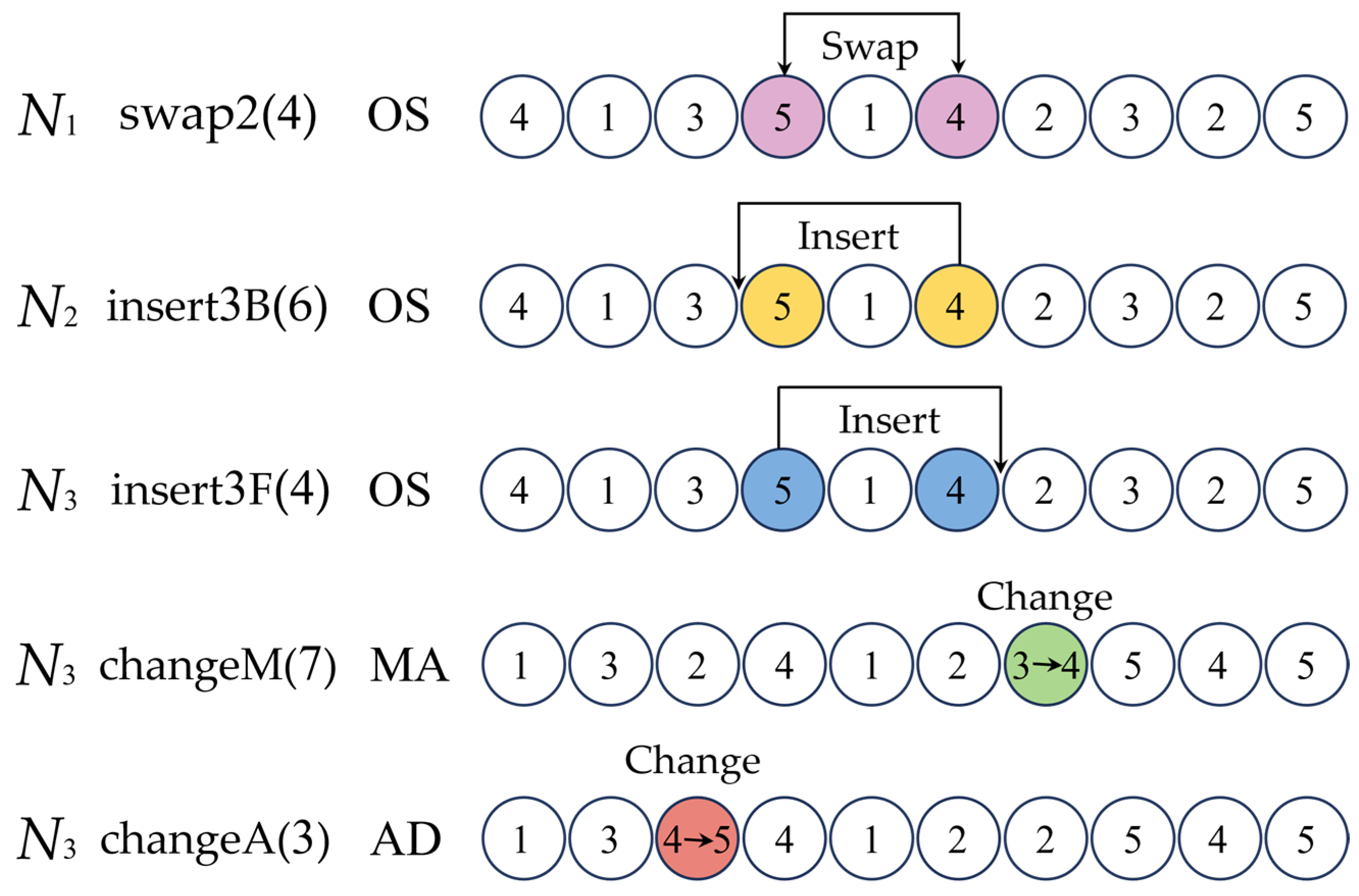
In the original ABC algorithm, onlooker bees follow employed bees to perform searches. The fitness of each individual is calculated as its search probability, and then a roulette wheel selection method is used to select individuals for neighborhood searches. The higher the fitness of an individual, the greater the probability of being selected. Calculating the search probability of an individual based on fitness values is only applicable to single-objective optimization. In this paper, the optimization has two objectives, making it unsuitable to use fitness values to calculate the search probability of individuals. To enhance search efficacy and diversification for the integrated FJSP-MTA, we embed a Variable Neighborhood Search (VNS) into the onlooker bee phase. Rather than a single random tweak, each onlooker bee explores a portfolio of neighborhoods around the critical path in a fixed order; upon improvement, the search restarts from the first neighborhood, otherwise it proceeds to the next, until a termination criterion is reached. This paper proposes new problem-specific neighborhood structures Nk (k = 1, 2, 3, 4, 5), as illustrated in Figure 8. The neighborhood structures include the following: Find the critical path and swap the operation between the i-th operation and the 2nd operation following it (swap2(i)). Find the critical path and insert operation from the 3rd operation to the i-th operation before it (insert3B(i)). Find the critical path and insert the operation from the i-th operation to the 3rd operation following it (insert3F(i)). Find the critical path and change the i-th selected operation to another eligible machine (change M(i)). Find the critical path and change the i-th AGV assigned to the associated transport task by switching to another AGV (change A(i)).
The changes in neighborhoods are as follows:
  • N1: swap2(i): randomly select an integer i  1 i l e n g t h O S 2 and swap the positions of the i-th operation and the (i + 2) th operation in the OS vector.
  • N2: insert3B(i): randomly select an integer i  1 i l e n g t h O S 3 and insert the i-th operation into the position of the (i − 3) th operation.
  • N3: insert3F(i): randomly select an integer i  1 i l e n g t h O S 3 and insert the i-th operation into the position of the (i + 3) th operation.
  • N4: changeM(i): randomly select an integer i  1 i l e n g t h M A and change from the optional machine set.
  • N5: changeA(i): randomly select an integer i  1 i l e n g t h A D and change from the optional AGV set.

4.7. Scout Bee Phase

The scout bee phase primarily serves to enhance the algorithm’s global search capability, preventing it from becoming trapped in local optima. Following both employed bee and onlooker bee searches, if an individual fails to improve solution quality after undergoing limited iterations, a new individual must be regenerated to maintain diversity within the population. The original ABC algorithm uses random initialization to generate an initial solution as the updated value for the individual. However, solutions produced by random initialization tend to be poor. To address this issue, a restart strategy is used in the scout bee phase. For each individual, a stagnation counter records consecutive non-improving iterations and is reset upon improvement. Once the counter reaches limit, the individual is replaced by a newly constructed one. The new solution is generated by randomized constructive initialization: the OS vector is drawn as a random permutation of the operations vector. The MS vector assigns each operation to a machine sampled uniformly from its feasible set defined in the machine feasibility table. And the AD vector is sampled uniformly from {1, …, nV}. After replacement, the objective fitness is re-evaluated and the stagnation counter is cleared, thereby preserving population size while restoring diversity and enabling the search to escape stagnation.

5. Experimentation

To test the effectiveness and superiority of the proposed Q-HMOABC algorithm, three sets of experiments were conducted, the results of which are reported in this section. First, the best set of parameters for the proposed Q-HMOABC was determined using the Taguchi orthogonal experiment. Subsequently, in order to validate the effectiveness of the Q-HMOABC algorithm, unconstrained multi-objective benchmark functions and benchmark instances used in the literature were selected. Ablation experiments were conducted to compare its performance against other variant algorithms. Last, comparative experiments were conducted with other state-of-the-art algorithms on the benchmark instances.
All experiments in this section were coded in Matlab2022a on Windows 10 Professional system with Intel(R) Core(TM) i7-12700 CPU, @2.10 GHz and 16 GB RAM hardware environment. All algorithms ran 20 independent times on each instance with the same stop criteria. Three metrics are used to measure the performance of the different algorithms: generation distance (GD), IGD, and HV. The calculation equations for these metrics can be found in [34]. The lower the GD or IGD value, the better the performance of the algorithm. In contrast, the greater the HV value, the better the performance of the algorithm.

5.1. Experimental Instances

To the best of our knowledge, there are currently no benchmark instances available for the FJSP-MTA. Therefore, based on the “job–machine” benchmark functions for [35], this paper made appropriate modifications to the layout matrix within them. These instances were renamed BU01-09 and DN01-10, which can be downloaded from https://fastmanufacturingproject.wordpress.com/2019/04/11/fjspt-instances/ (accessed on 5 October 2025). The benchmark instances were categorized into two groups: small-scale and large-scale, respectively. For ATEC, the AGV’s empty power was set to 0.9 and 1.1, while loaded power was set to 2.2 and 1.8.

5.2. Experimental Parameters

In this section, a Taguchi approach to the design of experiment (DOE) [36] is adopted to obtain the best combination of parameters. The Q-HMOABC has six parameters, namely population size ps, learning rate α, discount factor γ, exploring rate ε, restarting number N, and number of VNS LS. Each parameter has three levels; each parameter appeared 36 times. The corresponding values are given as follows.
(1)
p s = 40 , 60 , 80 .
(2)
α = 0.05 , 0.1 , 0.15 .
(3)
γ = 0.7 , 0.8 , 0.9 .
(4)
ε = 0.3 , 0.5 , 0.7 .
(5)
N = 20 , 30 , 40 .
(6)
L S = 5 , 10 , 15
An orthogonal array L 18 ( 3 6 ) was adopted in this calibration experiment, and for fairness, the max generation G = 150. The mean values of 20 repeated times are shown in Table 3. Figure 9a shows the main effects plot of six parameters for the IGD metric, and Figure 9b shows the signal-to-noise ratio (S/N) corresponding to the IGD response. The lower the IGD metric values, the better the performance. Based on comprehensive observation, the best parametric value configuration was p s = 60 , α = 0.10 , γ = 0.7 , ε = 0.7 , N = 20 , and L S = 15 .

5.3. Effectiveness of Each Improvement of Q-HMOABC

In this section, ablation experiments were conducted to validate the effectiveness of the proposed Q-HMOABC algorithm against three variant algorithms demonstrate its effectiveness: Q-HMOABC-E, which excludes the RL mechanism in employed bee phase; Q-HMOABC-O, which excludes the VNS in onlooker bee phase; and Q-HMOABC-S, which excludes the restart strategy in scout bee phase.

5.3.1. Effectiveness of Q-HMOABC on Unconstrained Benchmark Functions

To test the performance of the Q-HMOABC algorithm, this section selected the unconstrained multi-objective benchmark functions widely used in the literature [37,38], ZDT3, ZDT4, and ZDT6, as two-objective optimization problems. DTLZ2 and DTLZ6 as three-objective optimization problems.
Table 4 presents the results of the Q-HMOABC-E, Q-HMOABC-O, Q-HMOABC-S, and Q-HMOABC optimization algorithms on five unconstrained benchmark functions for the IGD metric, including mean, maximum (Max), minimum (Min), and standard deviation (Std) values, with the optimal values indicated in bold. As shown in Table 4, the Q-HMOABC algorithm demonstrates superior distribution performance compared to the other three algorithms for the vast majority of functions. However, for the DTLZ2 function, the Q-HMOABC-S algorithm exhibits slightly superior distribution performance compared to the other algorithms. For the ZDT4 and DTLZ5 functions, Q-HMOABC demonstrates obviously superior performance over the other algorithms, proving that the proposed Q-HMOABC not only performs better at the convergence metric level but is also superior at the distribution metric level.
Table 5 presents the results for the five standard functions optimized by Q-HMOABC-E, Q-HMOABC-O, Q-HMOABC-S, and Q-HMOABC on the GD metric, also including the five values mentioned above. The best values are indicated in bold. Table 5 demonstrates that the optimal values are obtained by Q-HMOABC. While its performance on functions ZDT3 and DTLZ2 is only slightly superior to the Q-HMOABC-S algorithm, the Q-HMOABC algorithm significantly outperforms the other three algorithms on functions ZDT4, ZDT6, and DTLZ5.

5.3.2. Effectiveness of Q-HMOABC on Benchmark Instances

To further evaluate the effectiveness of the proposed Q-HMOABC, this section tests the performance of the Q-HMOABC algorithm against three other variant algorithms on benchmark instances. Table 6 records the mean and best values of the HV among all variant algorithms in all benchmark instances. The best values are indicated in bold. It can be seen that in terms of both the values of best and mean, Q-HMOABC was better than other three variant algorithms for 16 instances.
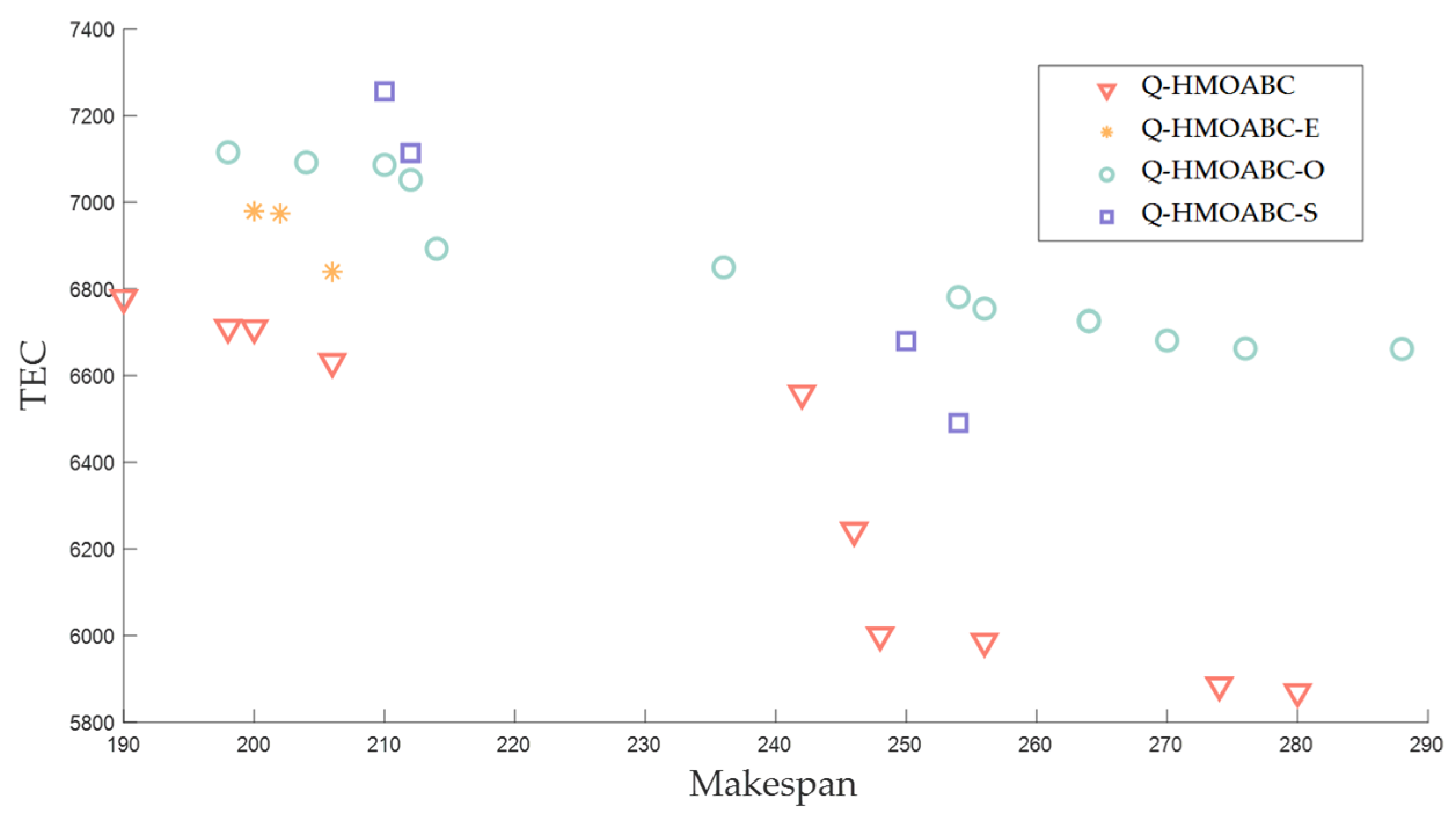
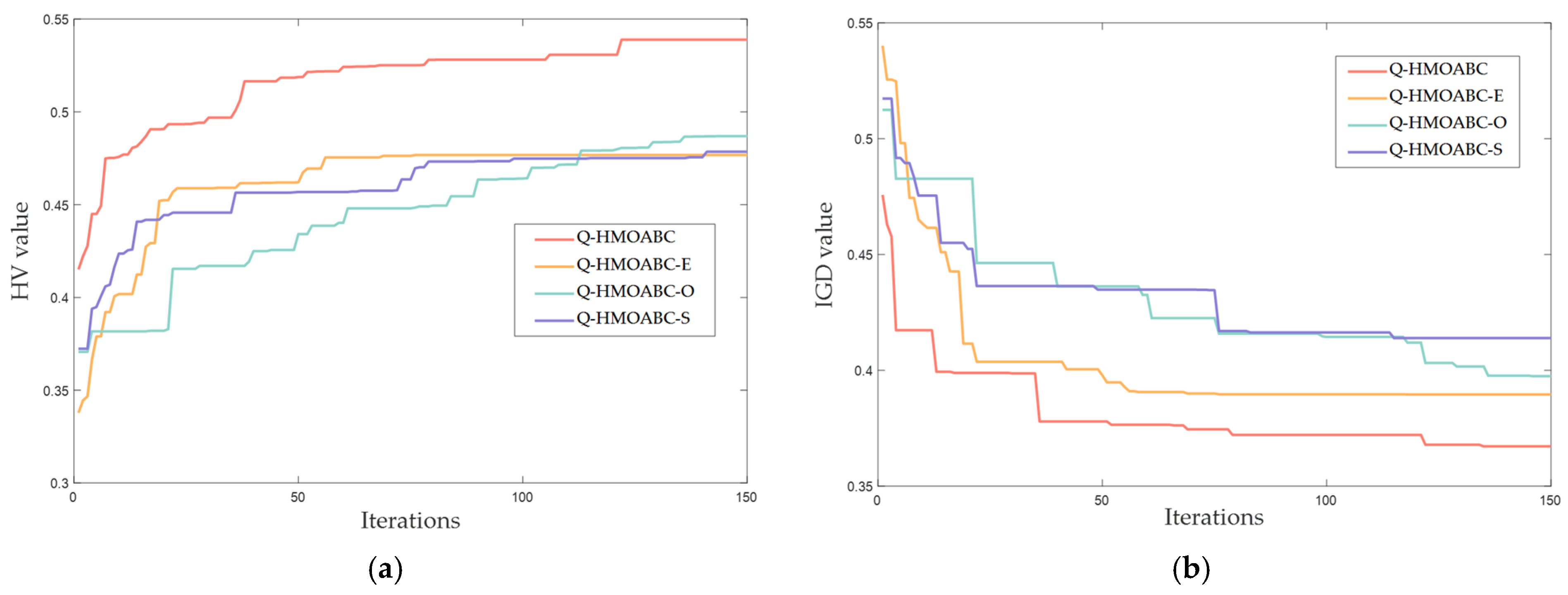
Figure 10 and Figure 11 illustrate the behavior of different algorithms on DN10. Figure 10 shows all algorithms’ Pareto front. Regarding the convergence and diversity of the Pareto front, Q-HMOABC can obtain better solutions than its variant competitors, which means Q-HMOABC can find closer approximations toward the real Pareto front. Meanwhile, we can see from Figure 10 that there is an obvious conflicting relationship between TEC and makespan. Figure 11a illustrates the performance trends of various algorithms on the HV metric after 150 iterations. It is evident that Q-HMOABC’s initial HV value surpassed that of other algorithms and maintained this lead throughout the iteration end. Similarly, it demonstrated optimal performance on the IGD metric, as shown in Figure 11b. As shown in the figures, Q-HMOABC demonstrated faster convergence and achieved superior final metrics values compared to the other three variant algorithms.
In conclusion, the design of Q-HMOABC demonstrated strong global search capability-ties. By utilizing improved strategies across three phases of the ABC, Q-HMOABC effectively explored the solution space of the FJSP-MTA, ensuring comprehensive optimization.

5.4. Comparison of Q-HMOABC with Other Algorithms

To further demonstrate the effectiveness and efficiency of Q-HMOABC, it is compared with state-of-the-art algorithms, namely the MOSSA [39], MOGWO [40], MOWOA [41], and NSGA-II [42]. The parameter settings for each of the aforementioned algorithms compared with Q-HMOABC were set to ps = 100, 120, 140. Additionally, NSGA-II is a well-known multi-objective algorithm. The parameter for it is set to ps = 120 in this section. The maximum iteration count (MIC) is set to 150 for all algorithms. The parameters of Q-HMOABC are configured as described in DOE testing. The comparative mean results of the experiment for HV metric are shown in Table 7, and the comparative mean results of the experiment for IGD metric are shown in Table 8. The mean runtime (in seconds) across all benchmark instances after each of the five algorithms ran independently 20 times is listed in the last row of the two tables. The best values are indicated in bold. Among the 17 benchmark instances, Q-HMOABC achieved 16 optimal mean values in HV, and 17 in IGD.
Additionally, the relative percentage increase (RPI) was employed for the ANOVA analysis of HV and IGD. The RPI is calculated using the following Equation (28):
R P I = V i V max V max × 100 %
where Vmax represents the maximum value of the performance metrics collected across the compared algorithms, and Vi denotes the performance metric value obtained by algorithm i. A paired t-test was also conducted at the 95% confidence level for the RPI values, with the results shown in Table 9. The p-values are less than 0.05, suggesting that Q-HMOABC is statistically superior to MOSSA, MOGWO, MOWOA, and NSGA-II.
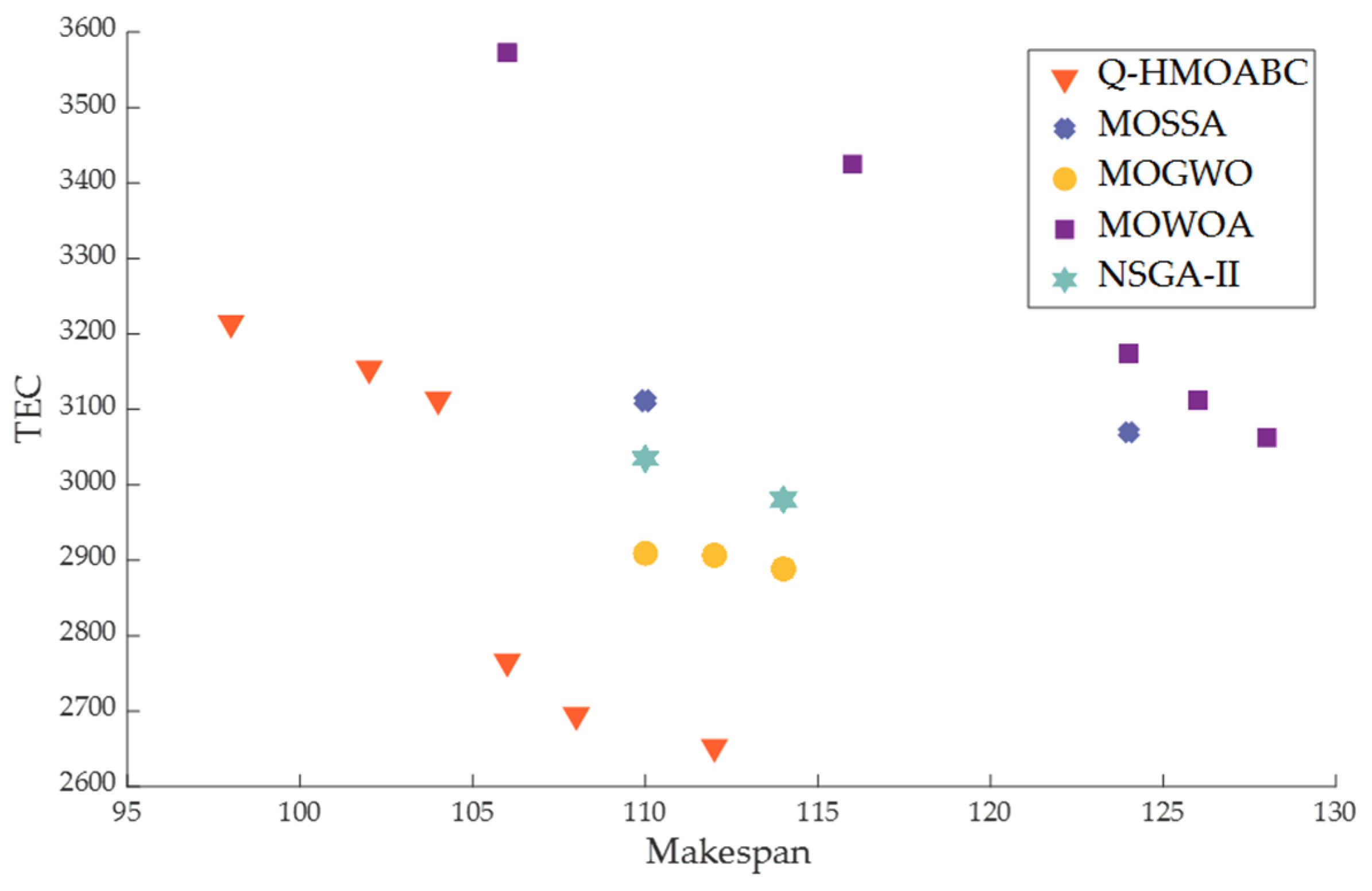
To illustrate the differences between the algorithms more intuitively, Figure 12 presents the Pareto front of DN05 obtained using different algorithms. The Pareto approximations show Q-HMOABC forming the leading frontier: its solutions occupy the lower-left region, with a smaller makespan and TEC. Other algorithms lie largely above this envelope, thus providing weaker trade-offs. Overall, Figure 12 indicates superior convergence and coverage of the true front by Q-HMOABC. From this Pareto front diagram, it can also be observed that at a makespan of around 110, the Q-HMOABC algorithm achieves approximately 2650 TEC in the DN05 case study, while the MOGWO algorithm achieves 2900 TEC. The TEC obtained by the other three algorithms is even higher. In addition, the performance metrics from 20 computations for each benchmark instance are illustrated as box plots in Figure 13, and the discrete points denote outliers. In Figure 13a, Q-HMOABC delivers higher HV than the other four algorithms. As shown in Figure 13b, Q-HMOABC obtains lower IGD than the competitors, indicating a closer and more uniform approximation to the Pareto front; NSGA-II occasionally reaches comparably low values. Overall, the results suggest that Q-HMOABC achieves a superior balance of convergence and diversity. These box plots clearly demonstrate that Q-HMOABC outperforms MOSSA, MOGWO, MOWOA, and NSGA-II in terms of optimal objective value and computation stability.
In conclusion, Q-HMOABC outperforms the existing state-of-the-art algorithms. It has a greater search ability for the solution space of the FJSP-MTA and three strategies across ABC phases that can provide better guidance to improve the search accuracy of the nondominated solutions.

6. Discussion

The experimental findings of this study extend beyond algorithmic superiority, offering broader implications for smart manufacturing. The explicit modeling of multi-type AGVs demonstrates that accounting for transporter heterogeneity is essential for accurately balancing production efficiency and energy consumption. Furthermore, the success of the Q-learning hybrid framework underscores the potential of creating more adaptive and autonomous optimization systems for complex scheduling.
However, several limitations affect the immediate industrial applicability of our work. While computationally superior to exact methods, our approach may still face challenges in very large-scale dynamic environments requiring real-time scheduling. More critically, the model incorporates several simplifying assumptions that limit its practical implementation. The exclusion of AGV battery constraints represents a particularly significant simplification, as it fails to capture the operational realities of AGV systems. Incorporating such power management considerations would inherently transform the problem into a more complex but practically relevant dynamic scheduling framework, where charging decisions must be continuously optimized alongside production tasks. This omission currently overlooks battery degradation, charging scheduling, and limited charging station resources. Without considering these constraints, our model may generate theoretically optimal but practically infeasible schedules due to power depletion during critical operations. Additionally, the deterministic nature of our model and its simplified energy consumption calculation—neglecting effects of acceleration, deceleration, and payload variations—further constrain its direct industrial application, highlighting the gap between our current framework and the stochastic conditions of actual manufacturing environments.

7. Conclusions and Future Research

Although the FJSP with AGV transportation resources has widely appeared in modern manufacturing, the FJSP with multi-type AGVs (FJSP-MTA) has been seldom researched. This work proposes a MILP model and Q-HMOABC for the FJSP-MTA with minimizing makespan and TEC. In Q-HMOABC, a three-layer encoding based on operation sequence, machine assignment, and AGV dispatching is used. Moreover, improvement strategies are employed across three phases of the Q-HMOABC algorithm: the employed bee phase integrated RL, the onlooker bee phase incorporated VNS, and the scout bee phase adopted a restart strategy, thereby enhancing the efficiency of solution space exploration. Ablation experiments are conducted on the unconstrained benchmark functions and benchmark instances. The comparison results prove that the three phases’ improvement strategy can more accurately approximate the true Pareto front. Similarly, comparative experiments are conducted with other state-of-the-art algorithms on benchmark instances, with performance metrics demonstrating the effectiveness of Q-HMOABC.
In future research, studies will focus on the following aspects. Firstly, additional constraints, such as sudden job insertion and AGV charging issues, will be incorporated during the modeling phase to further enhance the applicability of the problem. Secondly, our proposed improvement strategies may not be suitable for larger-scale benchmark instances. We will design an effective evolutionary strategy for the FJSP-MTA to improve the algorithm’s efficiency further and validate it on more complex benchmark instances. We will conduct a sensitivity analysis to systematically evaluate the effects of key parameters and guide their tuning in diverse industrial settings. Finally, swarm intelligence optimization represents a prominent area of contemporary research. Investigating whether multi-population coevolution can improve the effectiveness and robustness of the algorithm about FJSP-MTA warrants further inquiry.

Author Contributions

Conceptualization, S.G. and H.Z.; methodology, S.G. and H.Z.; formal analysis, S.G.; writing—original draft preparation, S.G.; writing—review and editing, S.G.; visualization, S.G. and Z.Y.; project administration, Z.X. All authors have read and agreed to the published version of the manuscript.

Funding

This work is supported by the Youth Program of the Basic Research Plan, Shenyang Institute of Automation, Chinese Academy of Sciences, under Grant 2023JC1K11; and in part by the Liaoning Provincial Natural Science Foundation, under Grant 2025-MS-084.

Institutional Review Board Statement

Not applicable.

Informed Consent Statement

Not applicable.

Data Availability Statement

Data will be made available on request.

Acknowledgments

We would like to acknowledge the anonymous reviewers and the editor for their suggestions, which improved the quality of this paper.

Conflicts of Interest

The authors declare no conflicts of interest.

Notations

NotationsDefinitions
Parameter:
IJob set. (I = 1, 2, 3, …, n)
JiOperation set of job i. (Ji = 1, 2, 3, …, ni)
KMachine set. (K = 1, 2, 3, …, m)
VTotal numbers of AGVs set. (V = 1, 2, 3, …, nV)
TTotal types of AGVs set. (T = 1, 2, 3, …, t)
VtNumber of AGVs of type t. (tT)
i, iJob indices.
j, jOperation indices.
v, vAGV indices, including all types of AGVs.
k, k′Machines indices.
Oi,jThe j-th operation of job i.
NTotal number of operations of all jobs.
nJob number.
mMachine number.
niOperation number of job i.
tAGV type indices.
nVTotal number of AGVs of all types.
K(i,j)Optional machine set for Oi,j.
PTi,j,kProcessing time of Oi,j on machine k.
TTk,k,tTransportation time of k and k′ type t AGV.
PPkProcessing power on machine k (kK).
I P k Idle power of machine k (kK).
A P e m p t y t The empty power of AGV t (tT).
A P l o a d t The load power of AGV t (tT).
TECTotal energy consumption in workshop.
MPECMachine processing energy consumption.
MIECMachine idle energy consumption.
ATECAGV total energy consumption.
MA large positive number.
Decision variable:
CmaxMakespan
Xi,j,k,t,vWhen Oi,j is processed on machine k and transported by AGV v of type t.
(Xi,j,k,t,v = 0, 1).
YMi,j,i,jWhen Oi,j is processed before Oi,j by the same machine.
(YMi,j,i,j = 0, 1).
YTt,v,i,j,i,jWhen Oi,j is transported before Oi,j by AGV v of type t.
(YTt,v, i,j, ij = 0, 1)
Si,jStart processing time of Oi,j.
SAi,j,t,vArrive time of AGV v of type t for transporting Oi,j.
EMkEnd processing time for machine k.
EAt,vEnd transporting time of AGV v of type t.

References

  1. Mareddy, P.L.; Narapureddy, S.R.; Dwivedula, V.R.; Karanam, P.R. Development of scheduling methodology in a multi-machine flexible manufacturing system without tool delay employing flower pollination algorithm. Eng. Appl. Artif. Intell. 2022, 115, 105275. [Google Scholar] [CrossRef]
  2. Kacem, I.; Hammadi, S.; Borne, P. Approach by localization and multiobjective evolutionary optimization for flexible job-shop scheduling problems. IEEE Trans. Syst. Man Cybern. Part C (Appl. Rev.) 2002, 32, 1–13. [Google Scholar] [CrossRef]
  3. Yan, J.; Liu, Z.; Zhang, C.; Zhang, T.; Zhang, Y.; Yang, C. Research on flexible job shop scheduling under finite transportation conditions for digital twin workshop. Robot. Comput.-Integr. Manuf. 2021, 72, 102198. [Google Scholar] [CrossRef]
  4. Pan, Z.; Lei, D.; Wang, L. A Bi-Population Evolutionary Algorithm With Feedback for Energy-Efficient Fuzzy Flexible Job Shop Scheduling. IEEE Trans. Syst. Man Cybern. Syst. 2022, 52, 5295–5307. [Google Scholar] [CrossRef]
  5. Saidi-Mehrabad, M.; Dehnavi-Arani, S.; Evazabadian, F.; Mahmoodian, V. An Ant Colony Algorithm (ACA) for solving the new integrated model of job shop scheduling and conflict-free routing of AGVs. Comput. Ind. Eng. 2015, 86, 2–13. [Google Scholar] [CrossRef]
  6. Xu, G.; Bao, Q.; Zhang, H. Multi-objective green scheduling of integrated flexible job shop and automated guided vehicles. Eng. Appl. Artif. Intell. 2023, 126, 106864. [Google Scholar] [CrossRef]
  7. Ahmadi-Javid, A.; Hooshangi-Tabrizi, P. Integrating employee timetabling with scheduling of machines and transporters in a job-shop environment: A mathematical formulation and an Anarchic Society Optimization algorithm. Comput. Oper. Res. 2017, 84, 73–91. [Google Scholar] [CrossRef]
  8. Dang, Q.-V.; Singh, N.; Adan, I.; Martagan, T.; van de Sande, D. Scheduling heterogeneous multi-load AGVs with battery constraints. Comput. Oper. Res. 2021, 136, 105517. [Google Scholar] [CrossRef]
  9. Huo, X.; He, X.; Xiong, Z.; Wu, X. Multi-objective optimization for scheduling multi-load automated guided vehicles with consideration of energy consumption. Transp. Res. Part C Emerg. Technol. 2024, 161, 104548. [Google Scholar] [CrossRef]
  10. Fontes, D.B.M.M.; Homayouni, S.M.; Fernandes, J.C. Energy-efficient job shop scheduling problem with transport resources considering speed adjustable resources. Int. J. Prod. Res. 2024, 62, 867–890. [Google Scholar] [CrossRef]
  11. Zhang, R.; Yu, H.; Gao, K.; Fu, Y.; Kim, J.H. A Q-learning based artificial bee colony algorithm for solving surgery scheduling problems with setup time. Swarm Evol. Comput. 2024, 90, 101686. [Google Scholar] [CrossRef]
  12. Ajani, O.S.; Ivan, D.F.; Darlan, D.; Suganthan, P.N.; Gao, K.; Mallipeddi, R. Deep reinforcement learning as multiobjective optimization benchmarks: Problem formulation and performance assessment. Swarm Evol. Comput. 2024, 90, 101692. [Google Scholar] [CrossRef]
  13. Wang, J.J.; Wang, L. A Cooperative Memetic Algorithm With Learning-Based Agent for Energy-Aware Distributed Hybrid Flow-Shop Scheduling. IEEE Trans. Evol. Comput. 2022, 26, 461–475. [Google Scholar] [CrossRef]
  14. Raman, N. Simultaneous scheduling of machines and material handling devices in automated manufacturing. In Proceedings of the Second ORSA/TIMS Conference on Flexible Manufacturing Systems: Operations Research Models and Applications, Ann Arbor, MI, USA, 12–15 August 1986. [Google Scholar]
  15. Bilge, U.; Ulusoy, G. A Time Window Approach to Simultaneous Scheduling of Machines and Material Handling System in an FMS. Oper. Res. 1995, 43, 1058–1070. [Google Scholar] [CrossRef]
  16. Ham, A. Transfer-robot task scheduling in flexible job shop. J. Intell. Manuf. 2020, 31, 1783–1793. [Google Scholar] [CrossRef]
  17. Pan, Z.; Wang, L.; Zheng, J.; Chen, J.F.; Wang, X. A Learning-Based Multipopulation Evolutionary Optimization for Flexible Job Shop Scheduling Problem With Finite Transportation Resources. IEEE Trans. Evol. Comput. 2023, 27, 1590–1603. [Google Scholar] [CrossRef]
  18. Meng, L.; Cheng, W.; Zhang, B.; Zou, W.; Fang, W.; Duan, P. An Improved Genetic Algorithm for Solving the Multi-AGV Flexible Job Shop Scheduling Problem. Sensors 2023, 23, 3815. [Google Scholar] [CrossRef] [PubMed]
  19. Han, X.; Cheng, W.; Meng, L.; Zhang, B.; Gao, K.; Zhang, C.; Duan, P. A dual population collaborative genetic algorithm for solving flexible job shop scheduling problem with AGV. Swarm Evol. Comput. 2024, 86, 101538. [Google Scholar] [CrossRef]
  20. Homayouni, S.M.; Fontes, D.B.M.M. Production and transport scheduling in flexible job shop manufacturing systems. J. Glob. Optim. 2021, 79, 463–502. [Google Scholar] [CrossRef]
  21. Homayouni, S.M.; Fontes, D.B.M.M.; Gonçalves, J.F. A multistart biased random key genetic algorithm for the flexible job shop scheduling problem with transportation. Int. Trans. Oper. Res. 2023, 30, 688–716. [Google Scholar] [CrossRef]
  22. Liu, Z.; Luo, Q.; Wang, L.; Tang, H.; Li, Y. The Low-Carbon Scheduling Optimization of Integrated Multispeed Flexible Manufacturing and Multi-AGV Transportation. Processes 2022, 10, 1944. [Google Scholar] [CrossRef]
  23. Zhang, F.; Li, R.; Gong, W. Deep reinforcement learning-based memetic algorithm for energy-aware flexible job shop scheduling with multi-AGV. Comput. Ind. Eng. 2024, 189, 109917. [Google Scholar] [CrossRef]
  24. Fontes, D.B.M.M.; Homayouni, S.M. Joint production and transportation scheduling in flexible manufacturing systems. J. Glob. Optim. 2019, 74, 879–908. [Google Scholar] [CrossRef]
  25. Zhang, G.; Hu, Y.; Sun, J.; Zhang, W. An improved genetic algorithm for the flexible job shop scheduling problem with multiple time constraints. Swarm Evol. Comput. 2020, 54, 100664. [Google Scholar] [CrossRef]
  26. Ren, Y.; Wu, S.; Chen, S.; Burdette, J.E.; Cheng, X.; Kinghorn, A.D. Interaction of (+)-Strebloside and Its Derivatives with Na+/K+-ATPase and Other Targets. Molecules 2021, 26, 5675. [Google Scholar] [CrossRef]
  27. Gao, K.Z.; Suganthan, P.N.; Chua, T.J.; Chong, C.S.; Cai, T.X.; Pan, Q.K. A two-stage artificial bee colony algorithm scheduling flexible job-shop scheduling problem with new job insertion. Expert Syst. Appl. 2015, 42, 7652–7663. [Google Scholar] [CrossRef]
  28. Dong, X.; Wan, G.; Zeng, P. A heuristic-assisted deep reinforcement learning algorithm for flexible job shop scheduling with transport constraints. Complex Intell. Syst. 2025, 11, 210. [Google Scholar] [CrossRef]
  29. Cheng, W.; Meng, L.; Zhang, B.; Gao, K.; Sang, H. Imitation Learning-Assisted Evolutionary Algorithm for Energy-Efficient Flexible Job Shop Scheduling Problem with Automated Guided Vehicles. IEEE Trans. Evol. Comput. 2025, 1–15. [Google Scholar] [CrossRef]
  30. Li, Y.; Liao, C.; Wang, L.; Xiao, Y.; Cao, Y.; Guo, S. A Reinforcement Learning-Artificial Bee Colony algorithm for Flexible Job-shop Scheduling Problem with Lot Streaming. Appl. Soft Comput. 2023, 146, 110658. [Google Scholar] [CrossRef]
  31. Xu, S.; Li, Y.; Li, Q. A Deep Reinforcement Learning Method Based on a Transformer Model for the Flexible Job Shop Scheduling Problem. Electronics 2024, 13, 3696. [Google Scholar] [CrossRef]
  32. Zhang, Z.-Q.; Wu, F.-C.; Qian, B.; Hu, R.; Wang, L.; Jin, H.-P. A Q-learning-based hyper-heuristic evolutionary algorithm for the distributed flexible job-shop scheduling problem with crane transportation. Expert Syst. Appl. 2023, 234, 121050. [Google Scholar] [CrossRef]
  33. Yang, Y.; Yang, M.; Anwer, N.; Eynard, B.; Shu, L.H.; Xiao, J. A novel digital twin-assisted prediction approach for optimum rescheduling in high-efficient flexible production workshops. Comput. Ind. Eng. 2023, 182, 109398. [Google Scholar] [CrossRef]
  34. Meng, L.; Zhang, C.; Zhang, B.; Gao, K.; Ren, Y.; Sang, H. MILP modeling and optimization of multi-objective flexible job shop scheduling problem with controllable processing times. Swarm Evol. Comput. 2023, 82, 101374. [Google Scholar] [CrossRef]
  35. Deroussi, L.; Norre, S. Simultaneous scheduling of machines and vehicles for the flexible job shop problem. In Proceedings of the International Conference on Metaheuristics and Nature Inspired Computing, Djerba, Tunisia, 28–30 October 2010. [Google Scholar]
  36. Van Nostrand, R.C. Design of Experiments Using the Taguchi Approach: 16 Steps to Product and Process Improvement. Technometrics 2002, 44, 289. [Google Scholar] [CrossRef]
  37. Zitzler, E.; Deb, K.; Thiele, L. Comparison of Multiobjective Evolutionary Algorithms: Empirical Results. Evol. Comput. 2000, 8, 173–195. [Google Scholar] [CrossRef]
  38. Deb, K.; Thiele, L.; Laumanns, M.; Zitzler, E. Scalable multi-objective optimization test problems. In Proceedings of the 2002 Congress on Evolutionary Computation. CEC’02 (Cat. No.02TH8600), Hilton, HI, USA, 12–17 May 2002; Volume 821, pp. 825–830. [Google Scholar]
  39. Li, Y.; Xu, R.; Yan, L.; Gu, S. Research on joint scheduling of AGVs and machines in multi-objective flexible job shop based on ISSA. Robot. Intell. Autom. 2025, 45, 314–325. [Google Scholar] [CrossRef]
  40. Wei, Z.; Yu, Z.; Niu, R.; Zhao, Q.; Li, Z. Research on Flexible Job Shop Scheduling Method for Agricultural Equipment Considering Multi-Resource Constraints. Agriculture 2025, 15, 442. [Google Scholar] [CrossRef]
  41. Zhang, T.; Wei, M.; Gao, X. Modeling an Optimal Environmentally Friendly Energy-Saving Flexible Workshop. Appl. Sci. 2023, 13, 11896. [Google Scholar] [CrossRef]
  42. Deb, K.; Pratap, A.; Agarwal, S.; Meyarivan, T. A fast and elitist multiobjective genetic algorithm: NSGA-II. IEEE Trans. Evol. Comput. 2002, 6, 182–197. [Google Scholar] [CrossRef]
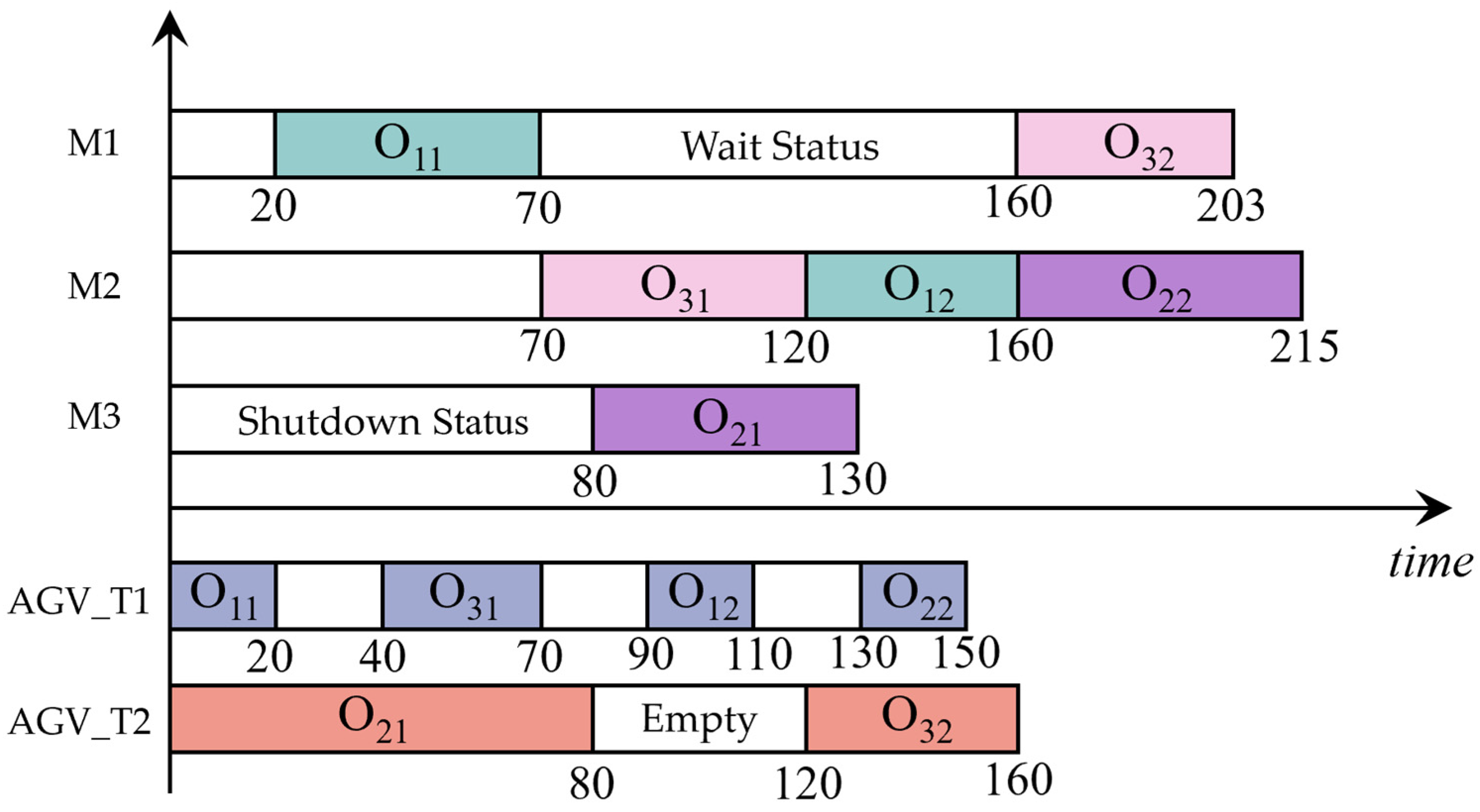
Figure 1. Gantt chart of a feasible schedule.
Applsci 15 10948 g001
Figure 2. Examples of the solution representation: (a) OS and (b) MA.
Applsci 15 10948 g002
Figure 3. An example of the AD solution representation.
Applsci 15 10948 g003
Figure 4. Example of PMX for OS genes.
Applsci 15 10948 g004
Figure 5. Example of POX for AD genes.
Applsci 15 10948 g005
Figure 6. The mechanism of RL.
Applsci 15 10948 g006
Figure 7. Examples of operators for action set. (a) IPOX, (b) TPX, (c) MPX.
Applsci 15 10948 g007
Figure 8. Five neighborhood structures of onlooker bee phase.
Applsci 15 10948 g008
Figure 9. (a) Main effects plot of IGD metric, (b) S/N corresponding to the IGD metric.
Applsci 15 10948 g009
Figure 10. Pareto front approximations by different variant algorithms on DN10.
Applsci 15 10948 g010
Figure 11. Iteration curve for metrics by different algorithms on DN10: (a) HV metric and (b) IGD metric.
Applsci 15 10948 g011
Figure 12. Pareto front approximations by different algorithms on DN5.
Applsci 15 10948 g012
Figure 13. Box plots of metrics for five algorithms: (a) HV metric and (b) IGD metric.
Applsci 15 10948 g013
Table 1. Cases of compatible machines/processing time of each operation.
JobOperationM1M2M3
Job 1O1,15062
O1,24055
Job 2O2,1554750
O2,26555
Job 3O3,1755043
O3,24352
Table 2. Transportation time between machines for two types of AGVs.
AGV_T1M0M1M2M3AGV_T2M0M1M2M3
M00203040M00406080
M1200 2030M1400 4060
M23020020M26040040
M34030200M38060400
Table 3. Mean of IGD value of BU09 different combination parameters.
TestParameterMean of IGD
psαγεNLS
1400.050.70.32050.38786
2400.10.80.530100.37171
3400.150.90.740150.36829
4600.050.70.530150.36577
5600.10.80.74050.37891
6600.150.90.320100.37141
7800.050.80.340100.37171
8800.10.90.520150.36714
9800.150.70.73050.38339
10400.050.90.730100.37181
11400.10.70.340150.36324
12400.150.80.52050.38538
13600.050.80.720150.36154
14600.10.90.33050.38859
15600.150.70.540100.36797
16800.050.90.54050.38515
17800.10.70.720100.36261
18800.150.80.330150.36585
Table 4. The comparison of the IGD metric on unconstrained benchmark functions.
FunctionsStatisticsQ-HMOABC-EQ-HMOABC-OQ-HMOABC-SQ-HMOABC
ZDT3Mean0.020870.032230.019790.01547
Max0.026210.037450.022950.01612
Min0.015940.026430.016250.01487
Std1.742 × 10−31.834 × 10−31.177 × 10−32.135 × 10⁻⁴
ZDT4Mean0.52581.77162.49997.327 × 10−3
Max0.58221.84092.83057.605 × 10−3
Min0.47101.68122.11647.018 × 10−3
Std0.03050.04370.19561.751 × 10−4
ZDT6Mean2.935 × 10−32.972 × 10−30.010292.025 × 10−3
Max3.054 × 10−33.103 × 10−30.015302.827 × 10−3
Min2.861 × 10−32.823 × 10−38.154 × 10−31.495 × 10⁻³
Std5.217 × 10−58.499 × 10−51.983 × 10−32.317 × 10⁻⁵
DTLZ2Mean0.095580.052510.051470.04958
Max0.120740.063070.058660.05940
Min0.061820.047300.043270.04129
Std0.016144.965 × 10−34.086 × 10−35.203 × 10−3
DTLZ5Mean0.029810.014310.011128.064 × 10−3
Max0.042050.027740.018968.237 × 10−3
Min0.025788.161 × 10−37.817 × 10−37.147 × 10−3
Std4.415 × 10−35.341 × 10−33.055 × 10−32.769 × 10⁻⁴
Table 5. The comparison of the GD metric on unconstrained benchmark functions.
FunctionsStatisticsQ-HMOABC-EQ-HMOABC-OQ-HMOABC-SQ-HMOABC
ZDT3Mean1.735 × 10−32.616 × 10−31.297 × 10−31.033 × 10−3
Max2.031 × 10−32.913 × 10−31.443 × 10−31.276 × 10⁻³
Min1.596 × 10−32.205 × 10−31.139 × 10−39.409 × 10⁻⁴
Std1.182 × 10−41.934 × 10−48.306 × 10−59.178 × 10⁻⁵
ZDT4Mean0.063600.21210.30299.217 × 10−5
Max0.091440.35130.45011.153 × 10−4
Min0.048010.12470.17738.592 × 10−5
Std9.866 × 10−30.055070.068458.024 × 10−6
ZDT6Mean0.077060.094190.077575.227 × 10−4
Max0.10430.13580.11327.905 × 10−4
Min0.059420.067030.064194.143 × 10−4
Std9.816 × 10−30.016250.013521.030 × 10−4
DTLZ2Mean9.264 × 10−32.215 × 10−31.810 × 10−31.614 × 10−3
Max0.012942.971 × 10−31.945 × 10−31.803 × 10−3
Min6.671 × 10−31.523 × 10−31.662 × 10−31.425 × 10⁻³
Std1.529 × 10−33.581 × 10−46.794 × 10−59.725 × 10⁻⁵
DTLZ5Mean2.832 × 10−31.340 × 10−31.207 × 10−33.538 × 10−4
Max3.281 × 10−31.736 × 10−31.553 × 10−33.910 × 10⁻⁴
Min2.394 × 10−31.039 × 10−39.835 × 10−42.968 × 10⁻⁴
Std2.018 × 10−41.909 × 10−41.431 × 10−42.164 × 10⁻⁵
Table 6. The comparison of the HV metric on benchmark instances.
InstancesQ-HMOABC-EQ-HMOABC-OQ-HMOABC-SQ-HMOABC
BestMeanBestMeanBestMeanBestMean
BU010.52370.50920.50040.49220.52140.50590.55930.5471
BU020.46740.45550.45280.44230.47020.46050.50120.4947
BU040.55870.53320.55740.51340.56470.52730.62830.5921
BU050.51290.50750.53100.51030.53820.51780.55990.5422
BU070.50960.48850.51270.47870.52090.50670.55560.5384
BU080.48280.45040.46140.42640.48370.44270.49670.4788
BU090.51140.50700.52160.50510.54920.52290.56550.5486
DN010.48310.46200.44370.42750.47560.46330.49690.4828
DN020.45230.44060.41140.39580.44190.42930.48890.4617
DN030.45900.44840.45400.41070.45270.43090.49300.4766
DN040.50840.48720.45060.42580.48300.46020.50500.4796
DN050.50560.47960.48360.44930.50200.47060.52070.5036
DN060.46020.43750.44100.41120.47630.44680.48640.4654
DN070.50080.48450.45680.43990.50740.48360.51900.4992
DN080.47240.45940.46740.43210.47270.45840.49210.4838
DN090.50780.49060.48710.45440.49010.48070.51860.5101
DN100.42730.41780.38950.38040.42690.40030.47850.4537
Table 7. Comparison of HV metric for Q-HMOABC, MOSSA, MOGWO, MOWOA, and NSGA-II on benchmark instances.
InstancesHV
Q-HMOABCMOSSAMOGWOMOWOANSGA-II
BU010.50510.39210.42450.40270.4525
BU020.50210.40130.41480.40460.4526
BU040.60630.45190.50240.44940.5423
BU050.55260.43320.46730.43900.5031
BU070.52170.42140.43740.40510.4643
BU080.55070.45350.47160.44290.5053
BU090.54250.42810.44490.42980.4979
DN010.51820.46260.47690.45330.4739
DN020.47410.40210.42230.40900.4284
DN030.47040.39340.43210.40170.4710
DN040.52420.41160.47030.41260.4916
DN050.51920.43540.46670.43060.4632
DN060.46650.39350.42940.39270.4225
DN070.48410.40980.43840.41240.4324
DN080.43600.37510.40260.38910.4104
DN090.49060.41230.43780.39960.4449
DN100.46350.38860.41000.38750.4064
Mean Runtime(s)714.6811.7761.2774.3730.5
Table 8. Comparison of IGD metric for Q-HMOABC, MOSSA, MOGWO, MOWOA, and NSGA-II on benchmark instances.
InstancesIGD
Q-HMOABCMOSSAMOGWOMOWOANSGA-II
BU010.38570.49120.45370.48610.4255
BU020.38630.48090.47160.47810.4176
BU040.28010.41890.36550.42280.3281
BU050.34760.44770.40640.44100.3744
BU070.36000.45680.43020.46560.4031
BU080.33180.41830.40190.42710.3701
BU090.34000.44410.42130.44220.3743
DN010.36090.41200.39730.42500.3953
DN020.43400.49350.46750.49510.4573
DN030.41950.48790.46010.47740.4394
DN040.34850.45870.39590.45740.3782
DN050.35660.44340.40100.44480.4072
DN060.44940.49670.46370.49870.4679
DN070.41090.47050.44940.46510.4442
DN080.44230.50080.48180.50200.4703
DN090.40590.47290.45560.47290.4358
DN100.43270.49570.46630.49210.4737
Mean Runtime(s)638.4733.9682.0706.2661.5
Table 9. Paired-t test for MOSSA, MOGWO, MOWOA and NSGA-II.
AlgorithmsHVIGD
Q-HMOABC vs. MOSSA0.0100.007
Q-HMOABC vs. MOGWO0.0060.010
Q-HMOABC vs. MOWOA0.0080.006
Q-HMOABC vs. NSGA-II0.0000.000
Disclaimer/Publisher’s Note: The statements, opinions and data contained in all publications are solely those of the individual author(s) and contributor(s) and not of MDPI and/or the editor(s). MDPI and/or the editor(s) disclaim responsibility for any injury to people or property resulting from any ideas, methods, instructions or products referred to in the content.