Diagnosing Hydraulic Directional Valve Spool Stick Faults Enabled by Hybridized Intelligent Algorithms

Abstract

The hydraulic directional valve represents a fundamental component of a hydraulic system. The severe operating environment could cause undesirable faults, with the spool stick being the particular concern. It will lead to a reduction in the overall performance of the operating system, even with the potential for failure. To address this issue, this study presents a hybrid intelligent algorithm-based diagnostic approach for the hydraulic directional valve spool stick fault to facilitate timely industrial inspection and maintenance. Firstly, the monitoring signals on hydraulic directional valves are denoised using wavelet packet denoising (WPD). Then, the denoised signals are decomposed via sparrow search algorithm (SSA) optimized for variational mode decomposition (VMD) in order to obtain a typical fault feature vector. Finally, a combined model of the convolutional neural network (CNN) and the long short-term memory (LSTM) is employed to diagnose the valve spool stick fault. The results of this study indicate that the proposed approach can reduce the signal processing time by 56.60%. The diagnostic accuracy of the approach is 97.01% and 96.24% for sensors located at different positions, and the accuracy of the fusion sensor group is 99.55%. These fault diagnostic performances provide a basis for further research into hydraulic directional valve spool stick fault and are appliable to other hydraulic equipment fault diagnosis applications.

1. Introduction

Hydraulic systems have been employed extensively in the operation of heavy-duty industrial machinery and manufacturing systems [1]. In hydraulic systems, directional valves are of critical importance as functional components. They are utilised for the purpose of regulating the direction and pressure of fluid flow [2]. In the context of practical applications, the occurrence of faults in hydraulic directional valves is particularly salient in environments characterised by elevated temperatures and humidity [3], vibration and shock [4], and extended periods of operation [5]. These conditions are conducive to the development of defects, underscoring the need for rigorous examination and mitigation strategies to ensure operational reliability and safety. It has been observed that a particularly prevalent fault is that of the spool stick. Consequently, the efficacy of hydraulic systems can be considerably diminished, with the potential to result in system failure in certain instances [6].

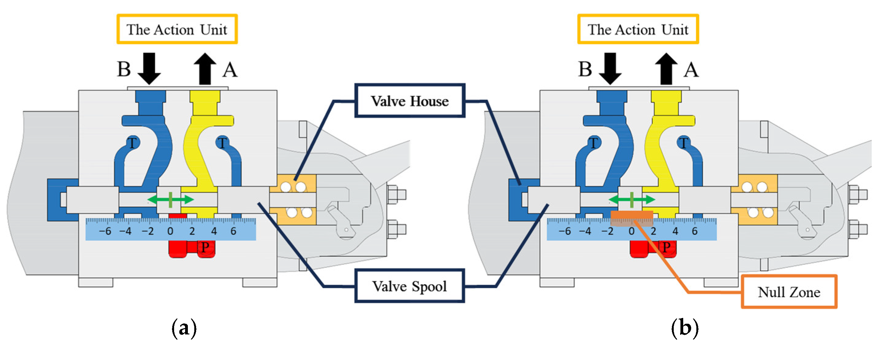
The proportional valve group 32 (PVG32) has been applied in various engineering fields [7]. The present paper will investigate the diagnosis of the PVG32 spool stick fault. The schematic diagram of the valve is presented in Figure 1. In accordance with the operational requirements, the handlebar is to be rotated in a clockwise direction, as illustrated in Figure 1a. Subsequently, the spool is shifted to the left side of the valve house, where the fluid is directed towards the action unit, thereby executing its designated power function.

It is conceivable that the occurrence of the valve spool stick fault may transpire during the operation of the valve (Figure 1b). For instance, the handlebar may be unable to rotate to the intended position due to the distortion of the valve inner wall after prolonged operation. This issue results in the valve spool being unable to move to its correct operating position and becoming stuck in the current situation. In such cases, the valve may supply an excess or deficiency of fluid to the action unit, which may result in an incorrect response to demands and even the failure of an entire system [8]. Therefore, a reliable diagnostic approach for the spool stick fault in hydraulic directional valves is required.

Data-driven methods employ data analysis techniques to achieve the goals of decision making, problem solving, and system development [9]. The application of these methods has been attempted in a variety of engineering contexts, including wind turbines, rotating machinery and rolling bearings. However, there is a paucity of published research on the diagnosis of hydraulic directional valve faults, particularly the spool stick.

The development of a data-driven diagnostic method to determine the spool stick fault of hydraulic directional valves is hindered by two main challenging issues. A significant challenge pertains to the procurement of adequate fault signals, a predicament exacerbated by the arduous nature of the working environment and the intricacy of the operating systems. A further challenge is posed by the temporal demands and the efficiency of the diagnostic process. Machine learning algorithms have been extensively utilised in various domains of fault diagnosis. Despite the capacity to intelligently extract the salient fault features with a view to providing effective support for fault diagnosis, the collected signals are frequently contaminated by ambient noise. This has the potential to compromise the performance of the algorithms.

In order to address the aforementioned issues, this paper presents a novel diagnostic approach that has been developed for the spool stick fault of the hydraulic directional valves. The proposed approach utilises a range of intelligent algorithms, including Wavelet Packet Denoising (WPD), Sparrow Search Algorithm (SSA), Variational Mode Decomposition (VMD), Convolutional Neural Network (CNN), and Long-Short Term Memory (LSTM). The primary contributions of this study can be enumerated as follows:

(1)

A hybrid signal processing framework (WPD-SSA-VMD) is proposed to enhance signal quality and processing efficiency. The WPD is initially employed for the denoising of raw vibration signals, followed by SSA-optimized VMD for the purpose of adaptive signal decomposition. This combination significantly reduces processing time while preserving essential fault features.

(2)

An integrated CNN-LSTM deep learning model has been developed to diagnose spool stick faults. This model has been developed by leveraging the strengths of both architectures. The utilisation of CNN (Convolutional Neural Network) is employed for the purpose of spatial feature extraction, whilst LSTM (Long Short-Term Memory) is utilised for the purpose of capturing long-range temporal dependencies in sequential vibration data.

(3)

A comprehensive evaluation system is established using three metrics: Model Accuracy (MA), Model Stability (MS), and Model Reliability (MR). A quantitative comparison and benchmarking against each other are conducted for these variables, utilising a 5-score ranking system. This enables a quantitative comparison and benchmarking of diagnostic performance across different models and sensor configurations.

Collectively, these contributions enable accurate, efficient, and reliable fault diagnosis for hydraulic directional valves, with potential applicability to other hydraulic systems.

The remainder of this paper is organized as follows. Section 2 provides a review of related works. Section 3 details the materials and methods. Section 4 presents and analyses the experimental results. Section 5 discussed the model parameter selection, the potential limitations and the corresponding future research. Finally, Section 6 concludes the paper.

2. Literature Survey

This section provides a review of the existing literature relevant to the methodologies employed in this study, thereby providing the necessary background and justifying the proposed hybrid approach. The review is structured into two main subsections. Firstly, signal processing techniques that are critical for the extraction of features are examined, with a particular focus on denoising and decomposition methods. Secondly, the paper explores machine learning and deep learning algorithms that form the basis of the diagnostic model. This structured review establishes the foundation for the integrated WPD-SSA-VMD and CNN-LSTM framework that is presented in this paper.

2.1. Signal Processing for Fault Diagnosis

A variety of signal processing methods have been developed and implemented in the field of fault diagnosis. Empirical mode decomposition (EMD) has gained considerable popularity as a signal processing method since it was first proposed in 1998 [10]. It can decompose non-linear and non-stationary signals adaptively in a manner different from traditional methods, such as the Fourier analysis and the filtering. Nevertheless, Lei et al. identified several limitations of EMD, including mode mixing, end effect, and stopping criterion [11]. Thus, Dragomiretskiy and Zosso developed the variational mode decomposition (VMD) as a novel method in 2013 to decompose any signal into a number of sub-signals in a more adaptive way [12]. The presence of a specific centre frequency and finite bandwidth in VMD enables it to circumvent the issues associated with EMD.

However, it should be noted that VMD requires the manual parameter selection, and that it is sensitive to the signal noise, which can affect the processing performance and efficiency. Therefore, VMD is usually employed in conjunction with the optimized algorithms to address the issues of the manual parameter selection. Jin et al. developed an improved grey wolf optimization algorithm for the VMD parameter selection, with the aim of identifying the weak bogie bearing faults of train axles [13]. The diagnostic accuracy was achieved by 96.7%. The method was based on manually extracted signal features, which limited its adaptability. Consequently, Li et al. applied the genetic algorithm to optimize the VMD parameters to diagnose faults in high-speed rolling bearings during their operational lifecycle [14]. Then, the optimized least squares support vector machine (SVM) was employed to identify fault features automatically, thus facilitating subsequent diagnostic procedures with an identification accuracy of 97%. The sparrow search algorithm (SSA) is an effective and novel optimization algorithm proposed by Xue and Shen in 2020 [15]. It was designed to simulate the anti-predation and foraging behaviour of the sparrow for optimization purposes. Xu et al. applied SSA to optimize VMD parameters to detect the face slab deflection, and its fitness function was designed with the value of the intrinsic mode function (IMF) and its corresponding centre frequency [16]. The validity of the proposed method was confirmed; however, it was determined that the optimisation procedure was time-consuming due to the extended signal length and the inadequate signal de-noising efficiency during the signal decomposition.

Consequently, denoising raw signals is a fundamental pre-processing step prior to the signal decomposition. WPD is one of the most effective strategies to address this issue [17]. Jiang et al. employed WPD and an improved adaptive neuro-fuzzy inference system to solve the issue of the electrical resistivity imaging (ERI) inversion [18]. The researchers utilized the Db10 wavelet function based on soft thresholding and Shannon entropy to remove the noise unit from their measured apparent resistivity data. Such a study could address two key problems of ERI inversion, i.e., the local minima and the overfitting. Beale et al. applied WPD to enhance the active acoustic damage detection of wind turbine blades [19]. The denoised signal resulted in a 60% enhancement in fault identification. These applications have been shown to provide a potential solution to the issue of the noise sensitivity associated with VMD, thereby improving the overall efficiency of the signal processing procedure.

In conclusion, the findings of this study indicate that the combination of these related methods may represent a potential avenue for obtaining a well-defined signal processing figure. In consideration of the signal pattern exhibited by the hydraulic directional valve spool in the present study, it is evident that WPD will be required to denoise the raw measured signals. Subsequently, the VMD technique will be utilised to decompose the de-noised signals, employing the SSA method to optimise the optimal parameter combination. In conclusion, the fault-related feature will be extracted for the subsequent application of the hydraulic directional valve spool stick fault diagnosis.

2.2. Deep Learning-Enabled Fault Diagnosis

Over the past few decades, machine learning algorithms have undergone rapid development, driven by the creation of powerful algorithms and the availability of large data sets. The support vector machine (SVM) is a supervised machine learning algorithm that can perform the classification and regression tasks. Zhang et al. combined the support vector data description and SVM with entropy-based features, which were investigated as indicators for the rotating machinery fault diagnosis [20]. The proposed method achieved over 94% fault detection accuracy. Nevertheless, SVM has several limitations that affect its widespread application in fault diagnosis. These include the low efficiency in handling with large datasets, the parameter selection sensitivity, and the interpretability [21]. Therefore, as an ensemble machine learning method, random forest (RF) has been applied to fault diagnosis due to the high interpretability and extensive input attributes of the tree-based model [22]. Mansouri et al. focused on the fault diagnosis in wind energy conversion systems by integrating Gaussian process regression and multi-class random forest [23]. The method illustrated the effectiveness of fault diagnosis with an overall identification accuracy of 99.94%.

The versatility of machine learning is further demonstrated in modern engineering systems that extend beyond traditional industrial machinery. To illustrate this point, consider the work of Marinković et al. [24], which explored the application of machine learning for digital twin techniques in the maintenance and exploitation of electric vehicles. The study under discussion highlights the potential of the aforementioned methods in predicting failures and optimizing maintenance schedules, thereby underscoring the cross-domain applicability of machine learning in complex system diagnostics.

However, these machine learning algorithms have the generalization issue when diagnosing faults under different conditions. Deep learning algorithms, including CNN and the recurrent neural network (RNN), have been widely employed in the fault diagnosis of mechanical systems due to their good ability to deal with complex input data and the high diagnostic accuracy. CNN is typically used to extract features from the sequential data and has been widely applied to the diagnosis of rolling bearing faults, as evidenced by the works of Guo et al. [25], Ruan et al. [26], and Zhao et al. [27]. In contrast, LSTM is a typical framework of RNNs, which is designed to sufficiently capture the long-range dependence of the sequential data [28]. An advanced algorithmic model has been proposed by Qin et al. to diagnose a wind turbine pitch system with multi-time sequence signal sources [29]. The utilisation of a long short-term memory (LSTM) network, equipped with a multi-channel attention mechanism, facilitated the identification of bearing and hub faults approximately 10 h prior to their occurrence, as documented by the wind farm. This outcome serves to substantiate the efficacy of the approach that was adopted.

Nevertheless, the limited ability of CNN to handle long-range dependencies in sequential data, and the LSTM challenge to capture long-term dependencies in sequential data, are two crucial obstacles to their further deployment in the fault diagnosis [30]. Thus, researchers have sought to integrate CNN with LSTM as a potential way to strengthen their characteristics for addressing complex tasks involving spatial and temporal dependencies. Xiang et al. have focused their research on the fault detection in wind turbines due to the complicated practical conditions involved [31]. The CNN model was integrated with the LSTM model as the proposed method to predict the early occurrence of faults and provide computable decision-making support. In addition, the CNN-LSTM model was used by Guo et al. for the hydraulic system fault diagnosis [32]. In this research, the strengths of CNN for feature extraction and LSTM for time series processing were combined. The model achieved an identification accuracy of 98.56% for different fault types.

In summary, the combination of CNN and LSTM models can be considered a viable method, given the diagnostic results and the strengths of the models in spatial features (processed by CNN) and temporal dependencies (processed by LSTM). In consideration of the characteristics of the hydraulic directional valve spool stick, the salient features are of a sequential nature with long-range dependence, rendering it well-suited for the implementation of a combined CNN-LSTM model for the purpose of fault diagnosis in the context of this study.

3. Materials and Methodologies

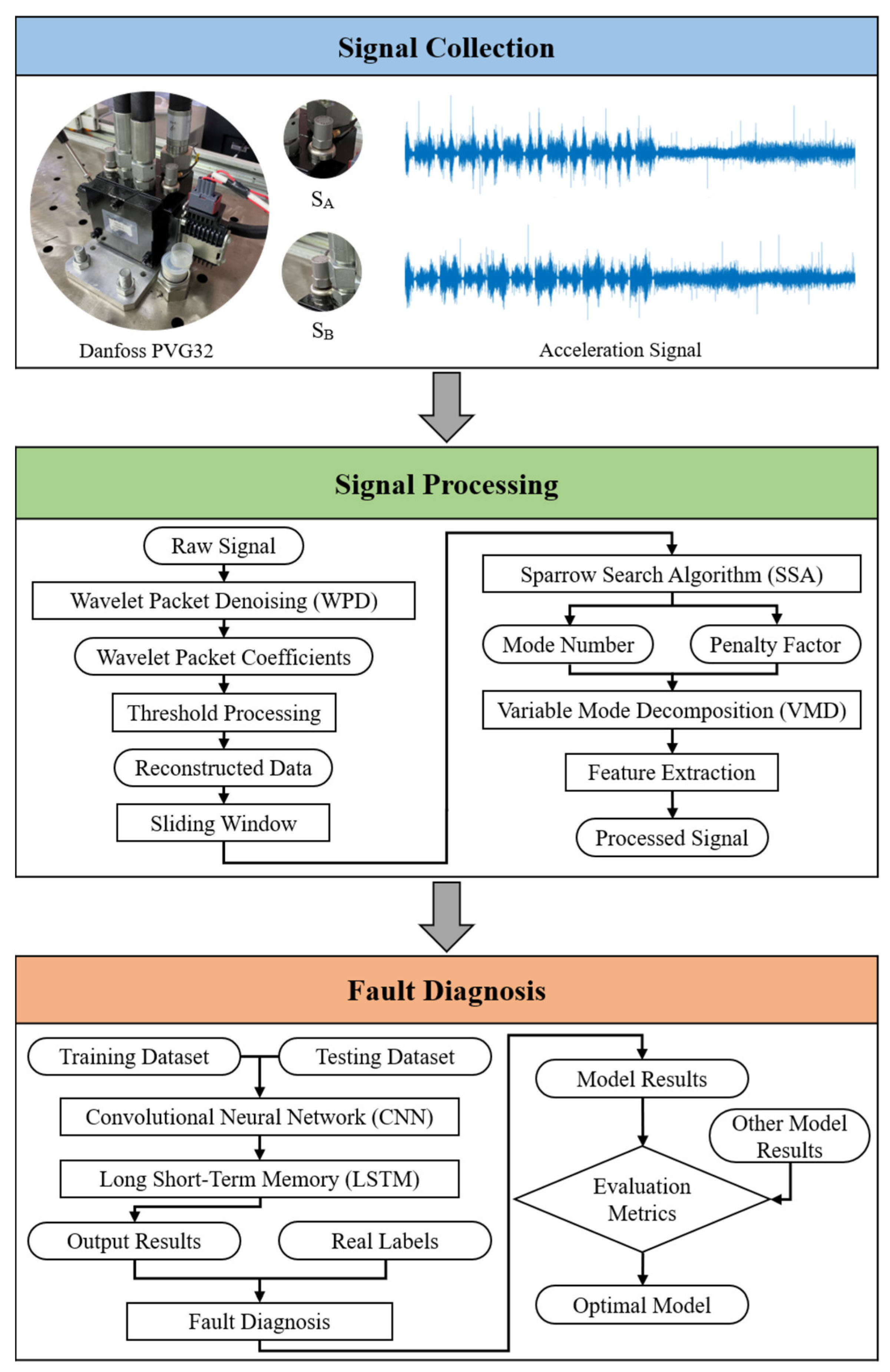
As demonstrated in Figure 2, the proposed research method (WPD-SSA-VMD-CNN-LSTM) comprises three primary procedures: signal collection, signal processing and fault diagnosis.

3.1. Signal Collection

3.1.1. Experimental Setup and Apparatus

In order to undertake a systematic investigation into the spool stick fault of the hydraulic directional valve, a dedicated experimental test rig was established on a Proportional Valve Group 32 (PVG32). The hydraulic system was configured to operate under a controlled load pressure of 0 MPa, with the objective of isolating the spool stick fault from pressure-induced effects. It was imperative that a constant pump drive speed of 1200 rpm was maintained in order to ensure consistent fluid flow throughout the duration of the experiments.

The primary data acquired for fault diagnosis were vibration signals, as they are highly sensitive to mechanical faults such as sticking spools. The employment of two high-sensitivity acceleration sensors (model: CT1010LC) was necessary in order to capture the aforementioned vibrational responses. The sensors were attached to two distinct ports (designated Port A and Port B) on the valve body, as illustrated in Figure 3. The employment of a dual-sensor configuration was instrumental in the documentation of potential asymmetrical vibration patterns. The induction of these patterns was attributed to the malfunction of the spool. The signals from these sensors were labelled S_A and S_B, respectively. The data acquisition system was configured with a sampling frequency of 4000 Hz [33]. This rate was selected to ensure the capture of the pertinent vibration frequency components associated with the valve’s operation, while maintaining an optimal data volume. As outlined in

Table 1. The experimental equipment and software.

Equipment	Software
Proportional Valve Group 32 (Danfoss, Nordborg, Denmark, Type PVG32)	Sign Collection: DAQami software (Version 3.0)
Acceleration Sensors (ICE Components, Marrieta, GA, USA, Type CT1010LC)	Signal Processing and Fault Diagnosis: MATLAB R2025a software (Version: v25.1.0.2943329)

the equipment and software utilised during the course of the experiments is enumerated.

3.1.2. Fault Simulation Methodology

The nominal operation of the valve involves the spool moving sinusoidally within a range of −7 mm to 7 mm inside the valve house, driven by a 0.01 Hz control signal (Figure 4a).

A critical preliminary step was the identification of the valve’s null zone. This is defined as the narrow range of spool displacement where minimal or no change occurs in the fluid flow and system pressure [34]. The zone as illustrated in Figure 4b was determined through empirical means to be between −2 mm and 2 mm for the valve under test [8]. This region is of particular interest as it has been observed that stiction faults often manifest when the spool attempts to traverse this critical area.

In order to simulate the occurrence of the spool stick fault, a deliberate intervention was performed. In contrast to the continuous movement characteristic of conventional valves, the present valve has been engineered to allow manual halting at a series of 11 predefined integral positions along its stroke. The strategic selection of these positions was undertaken to ensure comprehensive coverage of the operational range, with a particular emphasis on the null zone. The following fault positions were identified: The following values are to be considered: −7 mm, −6 mm, −5 mm, −4 mm, −3 mm, the null zone (approximated as the stuck position within −2 mm and 2 mm), 3 mm, 4 mm, 5 mm, 6 mm, and 7 mm.

At each of these positions, the spool was forcibly held, simulating a “stuck” condition. Subsequently, vibration data (signals S_A and S_B) were collected over a sufficient duration under this fault state. The process yielded a comprehensive dataset encompassing both normal movement and various fault scenarios. Consequently, this facilitated the identification of not only the occurrence of a stick fault, but also the precise position at which the spool was stuck.

3.2. Signal Processing

3.2.1. Wavelet Packet Denoising

WPD is based on the wavelet packet decomposition and the threshold denoising technique. Therefore, the WPD process can be divided into three general steps:

(1)

The signal decomposition:

Wavelet packet decomposition represents an enhanced form of wavelet transform that simultaneously decomposes the signal into low- and high- frequency sub-signals. This method can improve the high frequency resolution of the signals under the investigation and the local time domain analysis performance [35]. Thus, the general wavelet packet decomposition can be described as follows:

$$\left\{\begin{array}{c}{f}_i^{2j}\left(t\right)=\sum h_{m-2n}{f}_{i+1}^j\left(t\right)\\ f_i^{2j+1}\left(t\right)=\sum g_{m-2n}{f}_{i+1}^j\left(t\right)\end{array}\right.$$

(1)

where $t$ is the discrete time series, $f$ is the coefficient component of the wavelet packet decomposition, $f_{i+1}^j\left(t\right)$ is the raw input signal, $f_i^{2j}\left(t\right)$ and $f_i^{2j+1}\left(t\right)$ are the high- and low-frequency sub-signals, $h_{m-2n}$ and $g_{m-2n}$ are the high- and low-pass filter coefficients, $m$ and $n$ are the number of the decomposed layer, and $i$ and $j$ are the number of the wavelet packet node.

(2)

The threshold processing:

The calculation of high-pass filter coefficients $h_{m-2n}$ threshold is based on the Shannon entropy, after which the coefficients are quantified to reduce noise signals with the calculated threshold. The Shannon entropy ($SE$) can provide the information about the uncertainty and the basis for judgement in the decision-making process [36], as summarized below:

$$SE=-\sum _{h=1}^N {sn}_{h}log({sn}_h)$$

(2)

where $N$ is the sub-signal number, ${sn}_h$ is the sub-signal normalized value.

(3)

The signal reconstruction:

The aim is to reconstruct the low-frequency sub-signals $\sum g_{m-2n}{f}_i^{2j+1}\left(t\right)$ by combining them with the quantified high-frequency sub-signals $\sum h_{m-2n}{f}_i^{2j}\left(t\right)$, in order to obtain the required denoised signal ${fd}_{i+1}^j\left(t\right)$:

$${fd}_{i+1}^j\left(t\right)=\sum h_{m-2n}{f}_i^{2j}\left(t\right)+\sum g_{m-2n}{f}_i^{2j+1}\left(t\right)$$

(3)

3.2.2. Variational Mode Decomposition

VMD, initially proposed by Dragomiretskiy and Zosso, has become a widely used signal decomposition method for non-linear and non-stationary signals [12]. The method of transforming the signal decomposition problem into the variational problem, which seeks to find the extrema of a function that is the minimum in VMD, and the treatment of the variational problem, are two main essences of VMD. The procedures of VMD are outlined:

(1)

The signal decomposition

The input denoised signal $fd\left(t\right)$ can be decomposed into $k$ modal functions $u_k\left(t\right)$, which are also named intrinsic mode functions (IMFs). Then, the mixed $u_k\left(t\right)$ is combined with the estimated centre frequency $e^{-jwkt}$. Thus, the variational problem can be constructed with constraints, where all IMF modal functions $u_k\left(t\right)$ are added to the denoised signal $fd\left(t\right)$:

$$\begin{array}{c}\underset{u_k,{\omega }_k}{min} =\left\{{\displaystyle \sum _k} {∥{\partial }_t\left[\left(\delta (t)+{\displaystyle \frac{j}{k}}\right)u_k(t)\right]e^{-j{\omega }_{k}t}∥}_2\right\}\\ s.t.{\displaystyle \sum _k} u_k(t)=fd\left(t\right)\end{array}$$

(4)

where $fd\left(t\right)$ is the input denoised signal, $k$ is the decomposed mode number, $u_k\left(t\right)$ is the $k^{th}$ decomposed modal function, $e^{-jwkt}$ is the estimated center frequency, and ${\omega }_k$ is the $k^{th}$ mode estimated center frequency, ${\partial }_t$ is the $t$ partial derivative of the existing signal, ${\delta }_t$ is the Dirac Delta function.

(2)

Dealing the variational problem

In order to deal with Equation (4), first, it transforms the augmented Lagrangian equation into Equation (5) This is done by using the Lagrangian multiplier $\gamma \left(t\right)$ and the quadratic penalty factor $\alpha$:

$$\begin{array}{c}L\left(\right\{u_k\},\{{\omega }_n\},\gamma )=\\ \alpha {\displaystyle \sum _k} {∥\partial t\left[\left(\delta (t)+{\displaystyle \frac{j}{\pi t}}\times u_k(t)\right)\right]e^{-j{\omega }_{k}t}∥}_2^2+\\ {∥fd(t)-{\displaystyle \sum _k} u_k(t)∥}_2^2+(\gamma (t),fd(t)-{\displaystyle \sum _k} u_k(t))\end{array}$$

(5)

Then, the alternating direction multiplier method (ADMM) is employed to iteratively calculate Equations (4) and (5), until the value meets Equation (6) with the iteration number being $num$. The convergence conditions are as follows:

$${\sum }_{num}{\displaystyle \frac{{\parallel u_k^{num+1}-u_k^{num}\parallel }_2^2}{{\parallel u_k^{num}\parallel }_2^2}}<\epsilon$$

(6)

where $num$ is the iteration number, $\epsilon$ is the convergence error.

Finally, the input denoised signal $fd\left(t\right)$ can be decomposed via VMD to obtain the finite number of intrinsic mode functions (IMFs):

$$fd\left(t\right)={IMF}_1+{IMF}_2+\dots +{IMF}_i$$

(7)

where $i=1,2,\dots ,n$ is decided by the decomposed mode number $k$ manually.

3.2.3. Sparrow Search Algorithm

SSA is a novel swarm intelligence optimization algorithm developed by Xue and Shen in 2020 [15]. The algorithm was designed by simulating the behaviours of the sparrows, with a typical focus on the foraging and anti-predation actions. Therefore, SSA is able to simulate the sparrow foraging process to identify an optimal solution to the problem. The rules of the algorithm and the equations of the updated sparrow location are introduced below:

(a)

Each sparrow has the potential to become a producer if it is able to find more suitable food sources. Meanwhile, the ratio of producers and scroungers remains constant throughout the entire population.

(b)

Producers tend to have high energy reserve levels, and forages or scroungers are being responsible for finding the rich food source.

(c)

Individuals start chirping as a warning alarm when the sparrow detects the predator. As soon as the value of this warning alarm exceeds a safe threshold, it will be necessary for the producers to lead all of scroungers to the other safe regions.

Thus, during each iteration based on rules (b) and (c), the producer location can be renewed as follows:

$${PX}_{i,j}^{{iter}_{current}+1}=\left\{\begin{array}{c}{X}_{i,j}^{{iter}_{current}}\cdot \exp \left({\displaystyle \frac{-i}{\alpha \cdot {iter}_{max}}}\right),if R_2<ST\\ X_{i,j}^{{iter}_{current}}+Q\cdot L,if R_2\ge ST\end{array}\right.$$

(8)

where ${iter}_{current}$ is the current iteration number, $j=1,2,\dots ,d$ is the variable dimensions required to be optimised, $X_{i,j}^{{iter}_{current}}$ is the value of the $i th$ sparrow with the $j th$ dimension in the iteration, ${iter}_{max}$ is the maximum iteration number, $\alpha \left(\alpha \in \left(0,1\right]\right)$ is a random number, $R_2 (R_2\in \left[0,1\right]$) is the warning value. $ST (ST\in \left[0.5,1\right])$ is the safe threshold value, $Q$ is a normal distributed random number, and $L$ is an $1\times d$ matrix where all elements inside are $1$.

When $R_2<ST$, the surrounding is considered safe to search as there is no immediate threat from predators. This allows producers to conduct extensive searches. Nevertheless, a number of sparrows are identified as predators. It is imperative that all sparrows in this population should disperse immediately to other safe districts when $R_2\ge ST$.

(d)

The higher-energy sparrows will become the producers, while some starving scroungers may fly to other districts in search of food rather than gain more energy in the current district.

(e)

Scroungers will always be followed by producers, who will find and supply the optimal food sources. However, numerous scroungers may persistently supervise these producers and even compete for their food, thereby increasing their predation rate on all sparrows.

According to rules (d) and (e), the revised scrounger location can be introduced as follows:

$$\begin{array}{l}S{X}_{i,j}^{{iter}_{current}+1}\\ =\left\{\begin{array}{c}Q\cdot \exp \left({\displaystyle \frac{X_{\mathit{worst}}^{{iter}_{current}}-X_{i,j}^{{iter}_{current}}}{i^2}}\right),i>{\displaystyle \frac{N}{2}}\\ X_p^{{iter}_{current}+1}+\left|X_{i,j}^{{iter}_{current}}-X_{producer}^{{iter}_{current}+1}\right|\cdot A^{+}\cdot L,\mathrm{o}\mathrm{t}\mathrm{h}\mathrm{e}\mathrm{r}\mathrm{w}\mathrm{i}\mathrm{s}\mathrm{e}\end{array}\right.\end{array}$$

(9)

where $N$ is the sparrow number, $X_{\mathit{worst}}^{{iter}_{current}}$ is the overall worst position, $X_{producer}^{{iter}_{current}+1}$ is the producer at the optimized position in the ${iter}_{current}+1$ iteration, $A$ is the $1\times d$ matrix with randomly assigned value of $1$ or $-1$ for each element inside the typical matrix, $A^{+}=A^t(A{A}^t{)}^{-1}$.

The $i th$ scrounger will obtain an unsatisfied fitness value and will commence starvation if $i>{\displaystyle \frac{N}{2}}$. Otherwise, if $i\le {\displaystyle \frac{N}{2}}$, the $i th$ scrounger has randomly found a foraging location that is close to the optimal location.

(f)

Approximately 10% to 20% of the sparrow population at the periphery of the district are aware of the potential danger, so that they immediately move to a safer district in search of a more favourable environment.

The initial sparrow locations are randomly generated among the population according to the rule (f), which can be expressed as follows:

$$X_{i,j}^{{iter}_{current}+1}=\left\{\begin{array}{c}{X}_{\mathrm{b}\mathrm{e}\mathrm{s}\mathrm{t}}^{{iter}_{current}}+\beta \cdot \left|X_{ij}^{{iter}_{current}}-X_{\mathrm{b}\mathrm{e}\mathrm{s}\mathrm{t}}^{{iter}_{current}}\right|,if f_i>f_b\\ X_{ij}^{{iter}_{current}}+K\cdot \left({\displaystyle \frac{\left|X_{ij}^{{iter}_{current}}-X_{\mathrm{w}\mathrm{o}\mathrm{r}\mathrm{s}\mathrm{t}}^{{iter}_{current}}\right|}{\left(f_i-f_w\right)+\epsilon }}\right),if f_i=f_b\end{array}\right.$$

(10)

where $X_{\mathrm{b}\mathrm{e}\mathrm{s}\mathrm{t}}^{{iter}_{current}}$ is the overall best location, $\beta$ is the normal distributed random number with a variance of 1 and the average of 0, corresponding to the controlled parameter, $k (k\in [-\mathrm{1,1}\left]\right)$ is the sparrow movement direction and the step-controlled factor, $f_b,f_w$ are the fitness values for the best and the worst locations, respectively, $f_i$ is the $i th$ sparrow fitness value, $\epsilon$ is the constant value set as the smallest number to avoid 0 appearing in the denominator.

The sparrow is situated at the periphery of the group and may be the target of predators when $f_i>f_b$. When $f_i=f_b$, the sparrow is stayed in the central location, where it is forced to stay close to others because of the awareness of the imminent danger.

3.2.4. VMD Parameter Optimization by SSA

The performance of VMD is significantly influenced by two key parameters: the quadratic penalty factor ($\alpha$) and the decomposed mode number ($k$). The conventional approach is to manually select these parameters based on experimental results or expert experience, which is often inefficient and suboptimal. Therefore, in this study, SSA is applied to adaptively optimize the parameters of VMD, i.e., $\alpha$ and $k$.

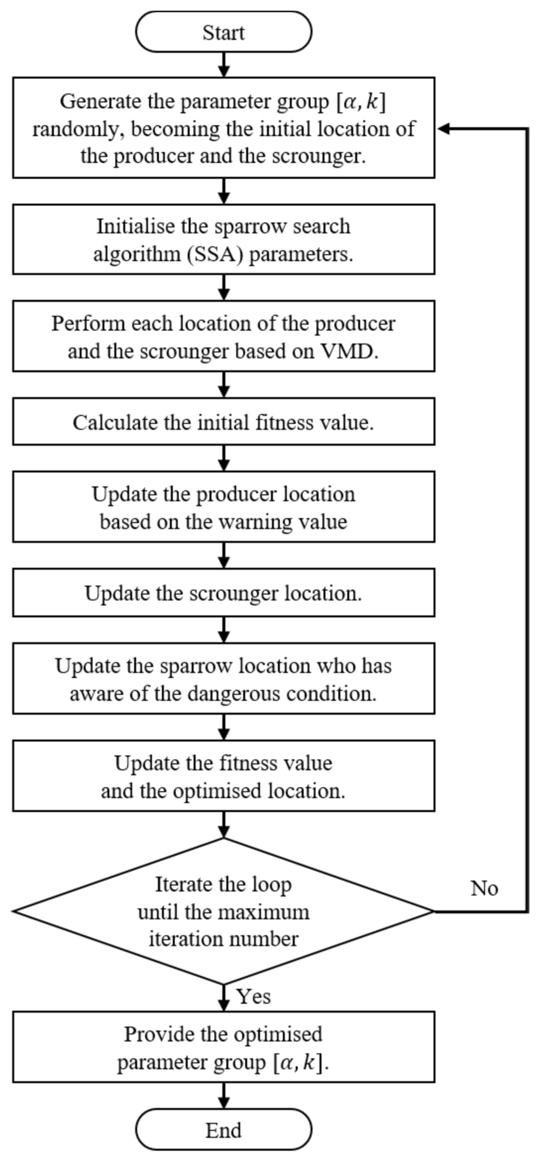
The general process of the SSA-optimized VMD is shown in Figure 5 and can be described in the following steps:

(1)

Initialization: The SSA population (sparrows) is initialized with each individual representing a potential solution, i.e., a combination of the VMD parameters [$\alpha$, $k$].

(2)

Fitness Evaluation: For each individual in the population, the VMD algorithm is run with its specific [$\alpha$, $k$] values to decompose the signal. The fitness of the solution is calculated as the envelope entropy of the resulting Intrinsic Mode Functions (IMFs). Envelope entropy serves as an effective fitness function because a lower value indicates less noise and more pronounced fault features in the decomposed components, which is desirable for effective feature extraction.

(3)

SSA Population Update: Based on the fitness evaluation, the positions of the producers, scroungers, and scouts are updated according to the SSA rules (as defined in Section 3.2.3). This step aims to guide the population towards the parameter combination that minimizes the envelope entropy.

(4)

Termination Check: The algorithm checks if the maximum number of iterations has been reached or if the fitness value has converged. If not, the process returns to Step 2.

(5)

Output Optimal Parameters: Once the termination condition is met, the best parameter combination [${\alpha }_{optimal}$, $k_{optimal}$] found by the SSA is output.

(6)

Final VMD: The denoised signal is finally decomposed using the VMD algorithm with the optimized parameters, yielding a set of high-quality IMFs for subsequent feature extraction.

This automated optimization process ensures that VMD is adapted to the specific characteristics of the input signal, leading to more robust and informative signal decomposition for fault diagnosis.

3.2.5. Feature Extraction

Considering the recorded signal characteristics of hydraulic directional valve spool stick faults, it can be posited that time domain features are sufficient for the fault diagnosis.

3.3. Fault Diagnosis

3.3.1. Convolutional Neural Network

CNN is a typical deep learning model with a shared weight network construction. The fundamental principle of CNN is the application of multiple filters, which are applied to extract features from the input data and classify or regress them [30]. A CNN model consists of an input layer, a convolutional layer with the activation function, a pooling layer, a fully connected layer with the SoftMax function, and an output layer.

3.3.2. Long Short-Term Memory

LSTM is an enhanced RNN that can examine the long- and short- term dependent messages to reduce gradient troubles during the model training process. It is able to handle time series data and fuse relevant features where CNN is unable to deal with such data types [32]. The general LSTM consists of three gates: an input gate, an output gate, and a forget gate.

3.3.3. Combination of CNN and LSTM

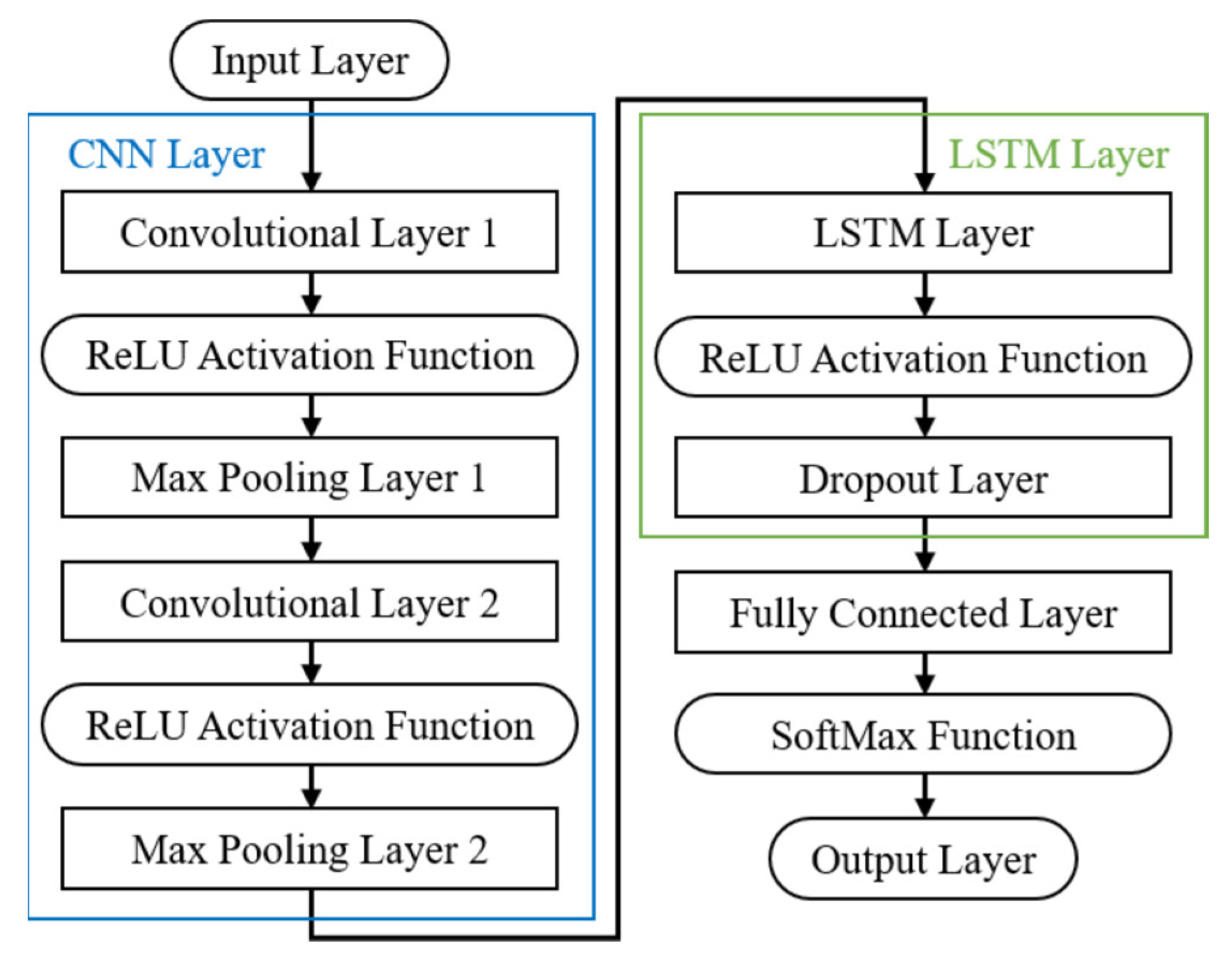
The integrated model of CNN and LSTM can be constructed for the purpose of diagnosing the hydraulic directional valve spool stick fault due to the sequential signal with long-range dependence features based on the signal processing and denoising procedure. Therefore, the potential combination of CNN and LSTM can leverage the respective strengths of each model, including the spatial feature extraction ability of CNN, the temporal advantage of LSTM, and the reduction in the overfitting issue. The flowchart of the CNN-LSTM model is illustrated in Figure 6, which contains the input layer, the CNN layer, the LSTM layer, the fully connected layer, and the output layer, respectively.

3.3.4. Evaluation Metrics

The objective of the evaluation metrics is to facilitate a comparative analysis of the diagnostic performance of different models. Then, a ranking system is employed to identify the optimal model for diagnosing the hydraulic directional valve spool stick fault in this study. Three indices are presented below:

(a)

Model Accuracy (MA): The average accuracy of four model training ratios (50%, 60%, 70%, and 80%) is presented to demonstrate the overall diagnostic accuracy of the model.

(b)

Model Stability (MS): The standard deviation of the diagnostic accuracy at different training ratios is used to reflect the model stability under different conditions.

(c)

Model Reliability (MR): The logarithm of the MA is calculated using the log base of the MS. The overall model reliability with different training ratios can be obtained for the further analysis of the optimization of the approach.

A ranking system has been used to compare the performance of different fault diagnostic models. The rank is on a scale of 1 to 5, where 5 is the best performance and 1 is the worst.

4. Results and Analysis

4.1. Signal Processing Approach

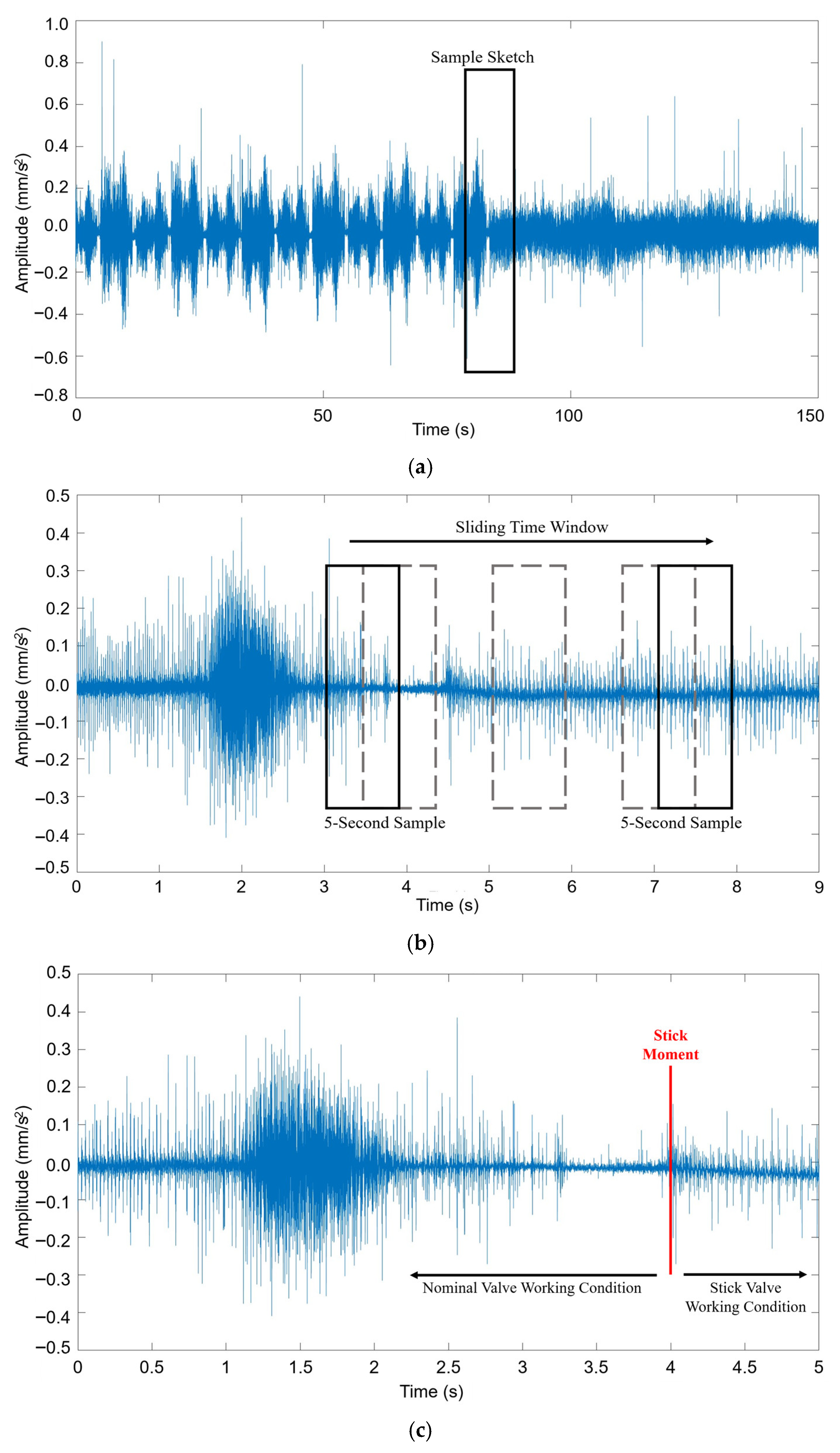
For each experimental condition (normal operation or a specific stick fault position), long-duration vibration signals were recorded. In order to facilitate the training of models and the subsequent analysis of the results, the sliding time window technique was applied to the raw signals. This method involves the extraction of numerous shorter, fixed-length samples from the continuous data stream. This process results in a substantial expansion of the size of the training dataset, thereby enhancing the model’s capacity to learn generalizable features. A window length corresponding to 20,000 data points was selected, providing a balance between capturing sufficient temporal information and maintaining computational efficiency. The pre-processing steps, from the original sample sketch to the final selected sample signals marked with the stick moment, are visually summarized in Figure 7.

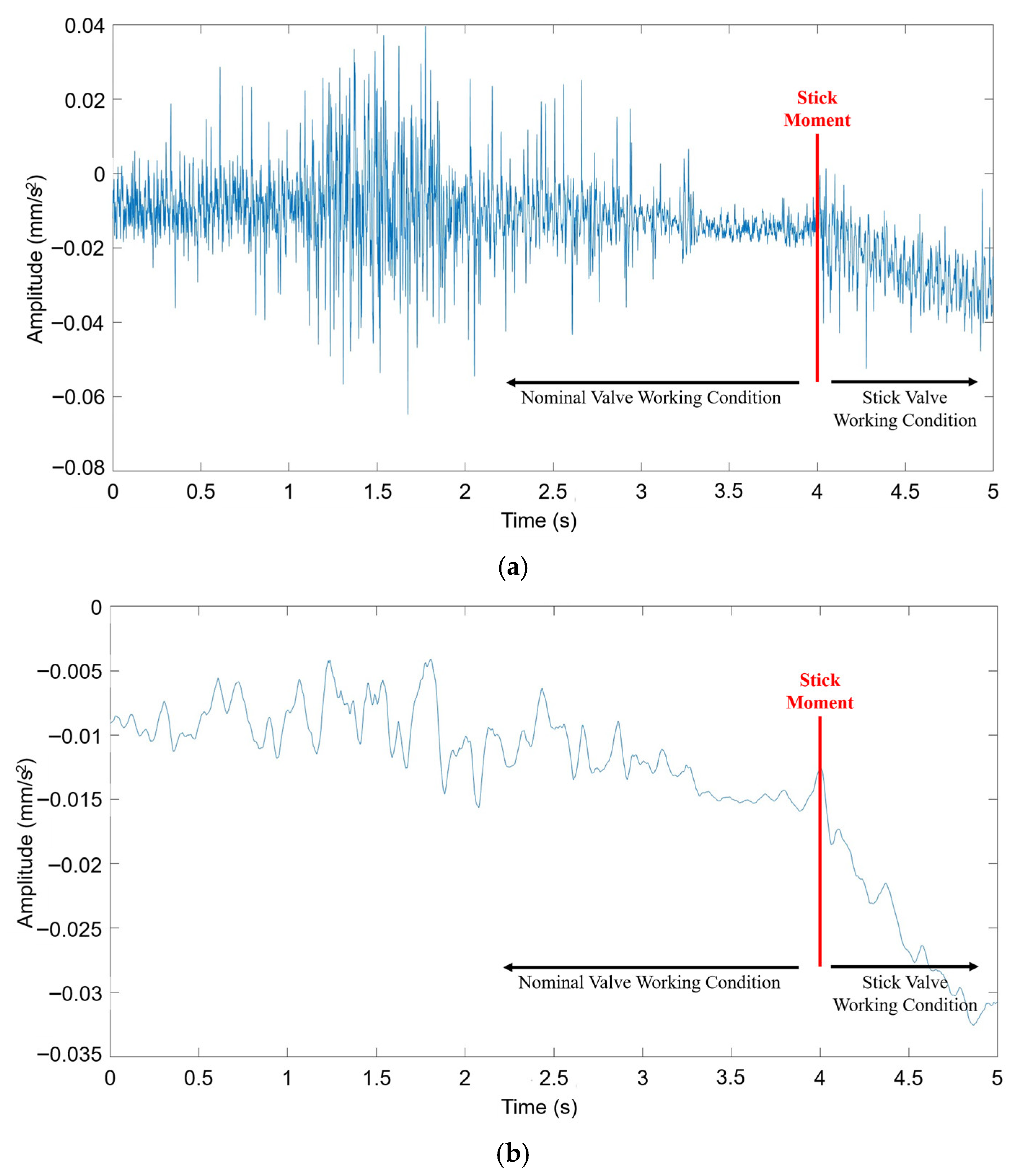
Figure 8 illustrates two signal processing approaches: SSA-VMD and WPD-SSA-VMD, respectively. In Figure 8a, the IMF has been obtained via VMD optimized by SSA. It is evident that the selected sample signals are subject to noise. However, WPD is applied prior to the SSA-optimized VMD, resulting in a significant denoising effect, as illustrated in Figure 8b. The processed signals show a sudden drop after the valve stick moment. Meanwhile, the optimal value of SSA in terms of fitness is applied to optimize parameters of the VMD, including the quadratic penalty factor ($\alpha$) and the decomposed mode number ($k$). As a result, the optimized parameter combination of VMD, i.e., 6046 of $\alpha$ and 19 of $k$, is identified with the lowest envelope entropy cost. It could represent the information uncertainty and the envelope randomness of the signals, and thereby it is advantageous for parameter optimized demands.

Further comparisons were made to demonstrate the need to apply WPD during the signal processing procedure.

Table 2. The results of signal processing approaches.

Approach	SSA-VMD				WPD-SSA-VMD
Ratio	50%	60%	70%	80%	50%	60%	70%	80%
SA	97.27%	98.79%	99.09%	99.70%	95.45%	96.67%	97.27%	98.64%
SB	97.27%	97.88%	98.18%	99.09%	95.15%	96.18%	96.36%	97.27%
SA & SB	99.64%	99.77%	100.00%	100.00%	99.09%	99.39%	99.70%	100.00%

and

Table 3. The comparisons of signal processing approaches.

Approach	SSA-VMD	WPD-SSA-VMD	Difference
SA	98.71%	97.01%	1.70%
SB	98.11%	96.24%	1.86%
SA & SB	99.85%	99.55%	0.31%
Time per Iteration	17,345.45 s	9818.18 s	56.60%

present the selected settings of the fault diagnosis model in this study, which are evaluated under four different model training ratios, 50%, 60%, 70% and 80%. Overall, the diagnostic results of both the signal processing approach, i.e., SSA-VMD and WPD-SSA-VMD, are above 95%. In all sensor groups, i.e., S_A, S_B, and S_A & S_B, the SSA-VMD approach showed superior accuracy levels compared to the WPD-SSA-VMD approach by 1.70%, 1.86%, and 0.31%, respectively. The average increase in accuracy is approximately 1.29% higher than that observed for the WPD-SSA-VMD approach. The visualization of the results showed that the WPD approach would slightly reduce the diagnostic accuracy as the denoising action could result in fewer fault features being filtered out of the signal. Nevertheless, it can be seen that WPD could save each iteration time for about 56.60% of the time spent per iteration of the VMD parameter optimization. The significant improvement in pre-processing efficiency offered by WPD is sufficient to justify the application of this validated strategy during the signal processing procedure. Concurrently, it could still be maintained a certain degree of diagnostic performance in the hydraulic directional valve spool stick fault.

Therefore, the signal processing approach employed in this study is identified as WPD-SSA-VMD. Firstly, the signals are processed by WPD. Then, the denoised signals are decomposed with SSA-optimized VMD. Finally, time domain features are extracted as a feature vector to support the diagnostic demand.

4.2. Fault Diagnosis Model

Five intelligent models are applied to select the optimal method, including SVM, RF, CNN, LSTM, and CNN-LSTM. Each model is trained with four ratios (50%, 60%, 70%, and 80%) and three sensor groups (S_A, S_B, and S_A & S_B). Therefore, the comprehensive performance is obtained in the diagnosis of the hydraulic directional valve spool stick fault. Consequently, the diagnostic results of the models as evaluated by the evaluation system and the 5-score ranking system are presented in

Table 4. The results of fault diagnosis models.

Sensor Group	SA				SB				SA & SB
Training Ratio	50%	60%	70%	80%	50%	60%	70%	80%	50%	60%	70%	80%
SVM	69.82%	70.68%	72.12%	73.18%	69.45%	70.91%	72.12%	73.64%	86.91%	87.05%	88.48%	89.55%
RF	93.27%	94.32%	94.55%	95.45%	92.27%	93.64%	94.45%	95.45%	97.82%	98.36%	98.79%	99.09%
CNN	94.18%	94.55%	95.15%	96.06%	94.18%	94.77%	95.15%	96.06%	98.36%	98.79%	99.09%	99.39%
LSTM	78.76%	79.64%	82.36%	83.64%	78.64%	79.27%	82.36%	83.18%	94.27%	95.59%	96.59%	97.64%
CNN-LSTM	95.45%	96.67%	97.27%	98.64%	95.15%	96.18%	96.36%	97.27%	99.09%	99.39%	99.70%	100.00%

and

Table 5. The analysis of fault diagnosis models.

Sensor Group	SA			SB			SA & SB			Rank
Index	MA	MS	MR	MA	MS	MR	MA	MS	MR	MA	MS	MR
SVM	71.45%	0.0129	0.0773	71.53%	0.0154	0.0803	88.00%	0.0109	0.0283	1.00	2.00	1.00
RF	94.40%	0.0078	0.0119	93.95%	0.0117	0.0140	98.52%	0.0048	0.0028	3.00	3.33	3.00
CNN	94.98%	0.0071	0.0104	95.04%	0.0068	0.0102	98.91%	0.0038	0.0020	4.00	4.67	4.00
LSTM	81.10%	0.0198	0.0534	80.86%	0.0194	0.0539	96.02%	0.0124	0.0092	2.00	1.00	2.00
CNN-LSTM	97.01%	0.0115	0.0068	96.24%	0.0075	0.0078	99.55%	0.0034	0.0008	5.00	4.00	5.00

.

In general, SVM shows the poorest performance across all sensor groups, with the highest MA observed in the S_A & S_B group, reaching 88%. The performance of RF and CNN is comparable, with differences in MA of around 1%. The LSTM model exhibits a 15% decrease in MA in both S_A and S_B sensor groups, and a 2% decrease in MA compared to the RF and CNN models in the S_A & S_B sensor group. However, the CNN-LSTM model achieves the highest MA performance among all models in S_A, S_B, and S_A & S_B, with the values of 97.01%, 96.24%, and 99.55%, respectively. In contrast, the MS value provides insight into the stability of the model, with a lower value indicating the greater stability. The CNN model exhibited the lowest MS values in two sensor groups (S_A and S_B), and the LSTM model shows the highest MS values. While the CNN-LSTM model obtains the most consistent performance across all sensor groups, in particular the S_A & S_B sensor group, which achieves the lowest value (=0.0034).

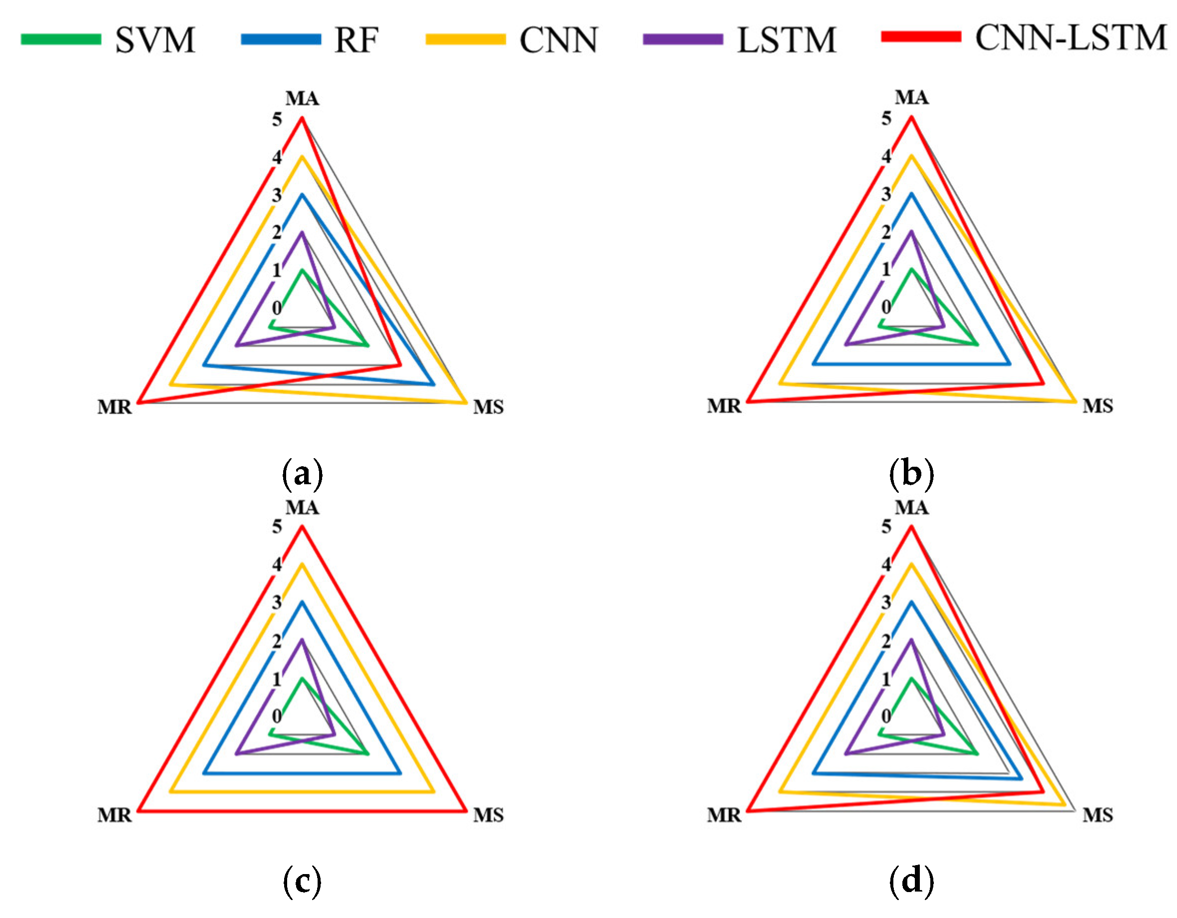
Furthermore, it is advisable to minimize the MR in order to ensure that the diagnostic model has the requisite generalization capacity under different training ratios (50%, 60%, 70% and 80%). Similarly to MA, CNN-LSTM achieves the lowest MR value among five models in three sensor groups, demonstrating the strengths of CNN and LSTM. Further procedures of the 5-score ranking system provide a clear picture of the model comparison, as shown in Figure 9.

The proposed fault diagnostic model, CNN-LSTM, shows the optimal performance as evidenced by the red solid line across almost all conditions. In particular, MA and MR are observed to be fully satisfactory. Only MS exhibits a slight decrease compared with the RF model as displayed in S_A sensor, and the CNN model performs well in S_A and S_B sensor groups. On the other hand, SVM and LSTM show suboptimal results, with scores of less than or equal to 2. Conversely, the RF model achieves the 3rd highest score among five models. The above comparisons motivate the integration of the CNN and LSTM models in this study. The CNN model is able to process the spatial data, while the LSTM model is able to process the sequential data over longer periods of time. However, the enhanced generalization capacity of the CNN-LSTM model is identified to be superior to that of the stand-alone models of either the CNN model or the LSTM model. Consequently, the fault diagnosis process begins with the input of fault features to the CNN model, which is then applied to the diagnosis of the final results by the LSTM model.

5. Discussion

5.1. Parameter Selection

The selection of appropriate model parameters is an important aspect that needs to be discussed to ensure that the proposed approach can maintain a certain level of efficiency and accuracy in diagnosing the valve spool stick fault. Therefore, a number of factors are considered, containing the LSTM cell, the CNN convolutional layer, and the kernels of each CNN convolutional layer, respectively. Each potential parameter is subjected to four training ratios with three groups of sensors, as previously described.

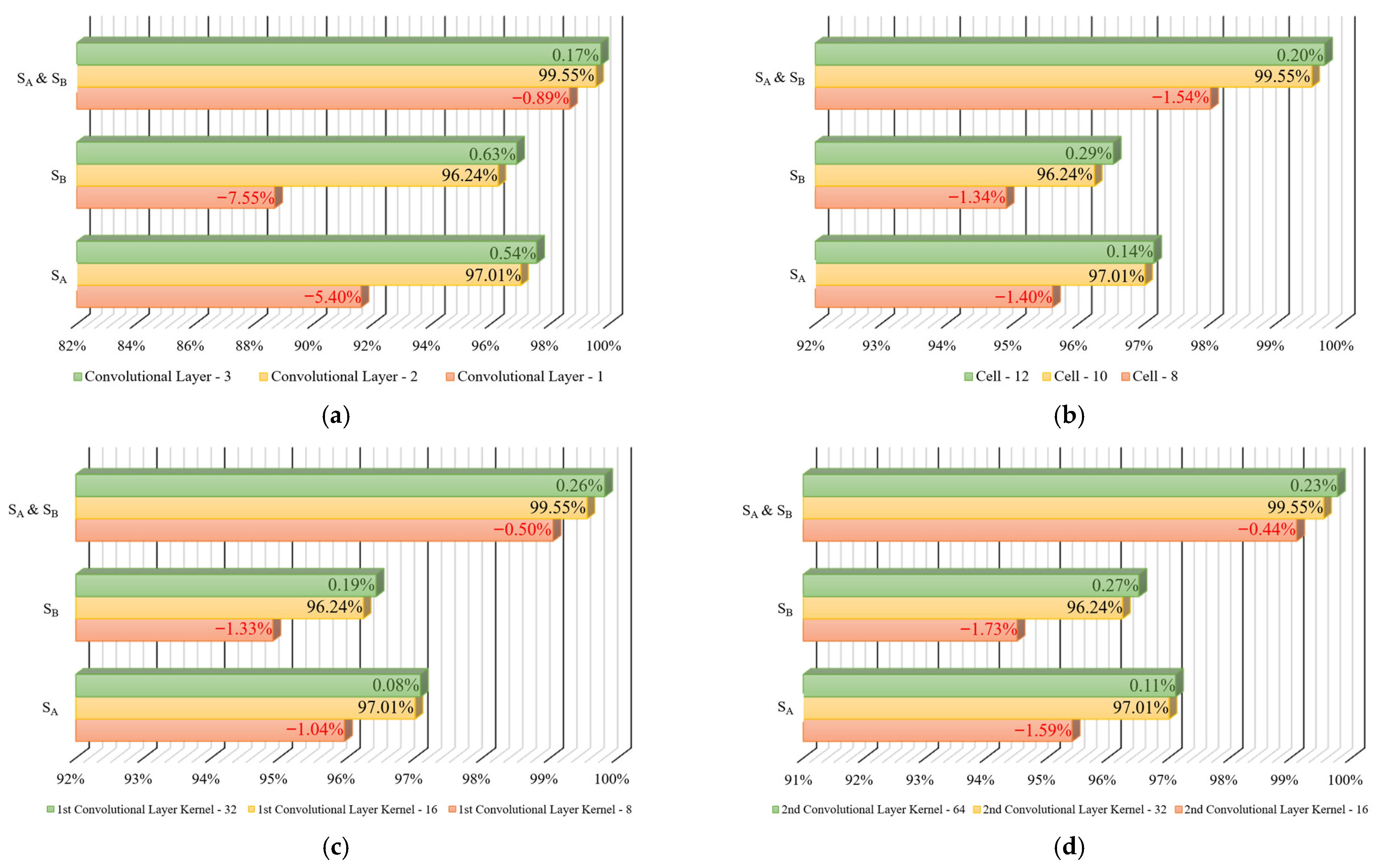
Each graph in Figure 10 is calculated based on the average fault diagnostic results. A percentage data label is proposed to reflect differences in results between parameters being compared. The green label represents a superior performance, while the red label represents an inferior performance in the same condition. In general, the larger the parameter value, the better the diagnostic performance.

Regarding to the number of the convolutional layers applied in Figure 10a, the model with a single convolutional layer is found to give unsatisfactory diagnostic results. The S_A and S_B sensor group values are observed to be 5.40% and 7.55% lower than those of the model with two convolutional layers. Although the model with three convolutional layers has the highest diagnostic accuracy, the overall increase is approximately 0.50% on average, with a minimum increase of 0.17% in the S_A & S_B sensor group. Similarly, the selection of the LSTM cell also shows similar patterns (Figure 10b). The smaller number of LSTM cells achieves a decline of over 1% compared to 10 cells, while the larger 12-cell configuration obtains a performance improvement of 0.20%. Based on the integrated comparison of accuracy changes, the two-convolutional-layer model with 10 LSTM cells is identified as the optimal candidate.

Considering the number of kernels in two convolutional layers, the likely parameters are determined to be 16 in the 1st convolutional layer and 32 in the 2nd convolutional layer. The largest reduction is observed in the 2nd convolutional layer with 16 kernels on the S_B sensor, with a decrease of 1.73%. The least improvement (0.08%) is observed in the 1st convolutional layer with 32 kernels at the S_A sensor. The overall increase in accuracy of both convolutional layers with different kernels is no greater than 0.30%. Thus, the use of larger kernels leads to higher levels of accuracy, but the benefits are limited, as shown in Figure 10c,d.

Furthermore, the time required for diagnosis is counted and presented in

Table 6. The fault diagnosing time of model parameters.

Model Parameters		Average Time (s)	Model Parameters		Average Time (s)
CNN Convolutional Layer	1	47.75	Kernels in 1st CNN Convolutional Layer	8	56.25
	2	58.00		16	58.00
	3	68.75		32	62.50
Model Parameters		Average Time (s)	Model Parameters		Average Time (s)
LSTM Cell	8	60.50	Kernels in 2nd CNN Convolutional Layer	16	56.00
	10	58.00		32	58.00
	12	59.25		64	62.75

to demonstrate the effectiveness of the model parameters under identical hardware and software conditions. Each value is the average time of all sensor groups with all training ratios, so that the generalization ability of the model can be detected among these parameters. It can be concluded that the smaller the value applied, the shorter the time cost. Nevertheless,

Table 7. The overall parameter comparisons.

Model Parameters		Accuracy Ratio	Time Ratio	Model Parameters		Accuracy Ratio	Time Ratio
CNN Convolutional Layer	1	−4.61%	−17.67%	Kernels in 1st CNN Convolutional Layer	8	−0.95%	−3.02%
	2	―	―		16	―	―
	3	0.45%	15.64%		32	0.18%	7.20%
Model Parameters		Accuracy Ratio	Time Ratio	Model Parameters		Accuracy Ratio	Time Ratio
LSTM Cell	8	−1.43%	4.13%	Kernels in 2nd CNN Convolutional Layer	16	−1.25%	−3.45%
	10	―	―		32	―	―
	12	0.18%	2.11%		64	0.20%	7.57%

calculates the rate change in the accuracy level and the diagnosis time. This allows a clear visualization of the overall difference and ensures that the most appropriate parameters can be rigorously and logically selected.

The substantial time difference is observed in the CNN convolutional layer. The single convolutional layer reduces the time cost by 17.67%, while three convolutional layers require 15.64% more time to complete the diagnostic procedure. The accuracy ratio of the single convolutional layer is reduced by 4.61%, while three convolutional layers exhibit an increase of 0.45%. Conversely, the time ratios of the kernel numbers in the convolutional layer are as expected. It is observed that the smaller kernel applied results in a shorter time spent, while the lower accuracy is obtained. Although the number of kernels is increased, resulting in a 0.20% improvement in diagnostic performance, the overall time cost is found to increase by 7.00%. In addition, the time required for smaller or larger LSTM cells is found to be longer, with a decline in accuracy ratio of 1.43% and an increase of 0.18%, respectively.

Thus,

Table 8. The final selected sufficient parameter.

Model Parameter	CNN Convolutional Layer	LSTM Cell	Kernels in 1st CNN Convolutional Layer	Kernels in 2nd CNN Convolutional Layer
Value	2	10	16	32

illustrates the final selected sufficient parameters for the CNN-LSTM model. The parameters ensure that the hydraulic directional valve spool stick fault diagnosis can achieve a certain level of efficiency and accuracy.

5.2. Potential Limitations

Notwithstanding the encouraging outcomes, it is imperative to acknowledge the study’s inherent limitations:

(1)

Computational Efficiency: Despite the incorporation of WPD leading to a significant reduction in signal processing time by 56.60%, the overall diagnostic process, particularly the SSA-optimized VMD and the CNN-LSTM model, remains computationally intensive. This may hinder the real-time application in industrial settings where computational resources are limited.

(2)

Generalization Ability: The model was subjected to training and validation procedures using a specific type of hydraulic directional valve (PVG32) within the confines of a controlled laboratory environment. However, the performance of the system under other valve types or under more varied and harsh real-world operating conditions (e.g., different fluid contaminants, temperature fluctuations, or pressure levels) remains unverified.

(3)

Sensor Dependency and Placement: The findings of this study demonstrated that the diagnostic accuracy was found to be sensitive to the sensor location. This was evidenced by a discrepancy in performance between the SA and SB sensor groups. This finding indicates that the model’s robustness may be influenced by the configuration of sensors in practical applications.

(4)

Feature Extraction Scope: The feature extraction process was predicated exclusively on time-domain features. While the inclusion of frequency-domain or time-frequency features was sufficient for the purposes of this study, the incorporation of such features could potentially capture more nuanced fault characteristics and further improve diagnostic robustness, especially with regard to incipient or compound faults.

5.3. Future Research

In order to address the aforementioned limitations and further advance the field, future research will focus on the following directions:

(1)

Multi-Sensor Information Fusion: Subsequent research endeavours will encompass the integration of supplementary sensor types, including pressure and temperature sensors. The objective of this integration is to develop a more comprehensive and robust array of fault features. It is hypothesised that this will enhance diagnostic accuracy and reliability to a greater extent than that achievable with vibration signals alone.

(2)

Model Lightweighting and Optimization: It is acknowledged that considerable effort will be expended on the development of lightweight versions of the diagnostic model. Such efforts may take the form of techniques such as model pruning, quantisation, or knowledge distillation. The objective of this approach is twofold: firstly, to reduce the computational burden, and secondly, to facilitate deployment in real-time embedded systems.

(3)

Transfer Learning and Generalizability: The present study will entail the execution of research, the objective of which is to apply transfer learning techniques. The implementation of these techniques will enable the pre-trained model to be adapted for the purpose of fault diagnosis in different types of hydraulic valves or systems with limited new data. It is hypothesised that the result of the adaptation process will be an enhancement in the generalisability of the model.

(4)

Enhanced Feature Extraction: The exploration of automated feature extraction, combining the time, frequency, and time-frequency domains using deep learning, will be pursued. Furthermore, the development of adaptive signal processing techniques capable of self-adjustment to varying noise levels and operational conditions is identified as a key objective.

6. Conclusions

This study has successfully developed and validated a hybrid intelligent framework for diagnosing spool stick faults in hydraulic directional valves. The conclusions presented herein are derived directly from the experimental results and discussions, synthesizing the key findings as follows:

(1)

The hybrid signal processing strategy (WPD-SSA-VMD) is of critical importance for achieving optimal diagnostic efficiency. In direct response to the challenge of computational cost, as discussed in Section 4.1, the integration of Wavelet Packet Denoising (WPD) as a pre-processing step was proven to be highly effective. The results presented in Table 2 offer quantitative evidence that this strategy led to a significant reduction in signal processing time per iteration by 56.60%, thereby decisively addressing the efficiency issue. This enhancement in processing speed was accompanied by a negligible yet valid trade-off in accuracy, with a reduction of approximately 1.29%, thereby validating the WPD-SSA-VMD as the optimal pre-processing pipeline for this specific application.

(2)

The CNN-LSTM model has been demonstrated to be the superior diagnostic architecture. The comprehensive model comparison in Section 4.2, evaluated using the MA, MS, and MR indices, conclusively demonstrated that the hybrid CNN-LSTM model outperformed all benchmark models (SVM, RF, CNN, LSTM). As outlined in Table 5 and Figure 9, the model demonstrated the highest Model Accuracy (MA) of 97.01% and 96.24% for individual sensors, and an impressive 99.55% for the fused sensor group. While its Model Stability (MS) was marginally lower than that of the CNN model in certain single-sensor scenarios, it exhibited the most consistent and reliable performance overall, as demonstrated by its superior Model Reliability (MR) scores. This finding serves to validate the design hypothesis that the combination of CNNs’ spatial feature extraction and LSTMs’ temporal modelling creates a more powerful diagnostic tool.

(3)

The selection of model parameters is directly linked to achieving a balance between accuracy and speed. The detailed discussion in Section 5.1 on parameter selection provides a clear rationale for the final model configuration. The selected parameters, comprising two convolutional layers, 10 long short-term memory (LSTM) cells, and kernel sizes of 16 and 32, were not chosen randomly but were empirically determined to offer the optimal compromise. As outlined in Table 7, this configuration circumvents the substantial 4.61% accuracy decline associated with a reduced model and the 15.64% temporal augmentation observed in a more substantial model. Consequently, it ensures diagnostic efficacy without incurring substantial computational overheads.

(4)

The fusion of multiple sensors has been demonstrated to significantly enhance the robustness of diagnostic systems. The findings consistently highlighted the benefit of utilizing multiple sensors. As demonstrated in Table 4 and Table 5, the fused S_A & S_B sensor group consistently demonstrated the highest levels of accuracy and the lowest levels of standard deviation across all models. The final CNN-LSTM model demonstrated an accuracy of 99.55%, substantiating the hypothesis that data from multiple valve ports provides a more comprehensive and robust fault signature.

In summary, the present research provides a validated, end-to-end solution for the spool stick fault diagnosis of hydraulic directional valves. The proposed WPD-SSA-VMD-CNN-LSTM framework has been demonstrated to be accurate, efficient, and robust. In future work, the limitations noted in Section 5.2, particularly regarding computational cost and generalization, will be addressed as the future research (Section 5.3) by exploring lightweight model designs and transfer learning techniques to facilitate real-world, industrial deployment.

References

1. Wang, J.; Yang, Z.; Liu, S.; Zhang, Q.; Han, Y. A comprehensive overview of hybrid construction machinery. Adv. Mech. Eng. 2016, 8. [Google Scholar] [CrossRef]
2. Quan, Z.; Quan, L.; Zhang, J. Review of energy efficient direct pump controlled cylinder electro-hydraulic technology. Renew. Sustain. Energy Rev. 2014, 35, 336–346. [Google Scholar] [CrossRef]
3. Kadar, F.; Hos, C.; Stepan, G. Delayed oscillator model of pressure relief valves with outlet piping. J. Sound Vib. 2022, 534, 117016. [Google Scholar] [CrossRef]
4. Awad, H.; Parrondo, J. Hydrodynamic self-excited vibrations in leaking spherical valves with annular seal. Alex. Eng. J. 2020, 59, 1515–1524. [Google Scholar] [CrossRef]
5. Simic, M.; Herakovic, N. Reduction of the flow forces in a small hydraulic seat valve as alternative approach to improve the valve characteristics. Energy Convers. Manag. 2015, 89, 708–718. [Google Scholar] [CrossRef]
6. Licsko, G.; Champneys, A.; Hos, C. Nonlinear analysis of a single stage pressure relief valve. Int. J. Appl. Math. 2023, 39, 286–299. [Google Scholar] [CrossRef]
7. Danfoss PVG 32 Proportional Valves. Available online: https://www.danfoss.com/en/products/dps/valves-and-actuators/valves/pvg-proportional-valves/pvg-32-proportional-valves (accessed on 10 September 2025).
8. Danfoss PVG 32 Proportional Valve Group Technical Information. Available online: https://assets.danfoss.com/documents/197489/BC152886483664zh-001401.pdf (accessed on 10 September 2025).
9. Gawde, S.; Patil, S.; Kumar, S.; Kamat, P.; Kotecha, K.; Abraham, A. Multi-fault diagnosis of industrial rotating machines using data-driven approach: A review of two decades of research. Eng. Appl. Artif. Intell. 2023, 123 Pt A, 106139. [Google Scholar] [CrossRef]
10. Huang, N.E.; Shen, Z.; Long, S.R.; Wu, M.C.; Shih, H.H.; Zheng, Q.; Yen, N.C.; Tung, C.C.; Liu, H. The empirical mode decomposition and the Hilbert spectrum for nonlinear and non-stationary time series analysis. Proc. R. Soc. A 1998, 454, 903–995. [Google Scholar] [CrossRef]
11. Lei, L.; Lin, J.; He, Z.; Zuo, M.J. A review on empirical mode decomposition in fault diagnosis of rotating machinery. Mech. Syst. Signal Process. 2012, 35, 108–126. [Google Scholar] [CrossRef]
12. Dragomiretskiy, K.; Zosso, D. Variational mode decomposition. IEEE Trans. Signal Process. 2014, 62, 531–544. [Google Scholar] [CrossRef]
13. Jin, Z.; He, D.; Wei, Z. Intelligent fault diagnosis of train axle box bearing based on parameter optimization VMD and improved DBN. Eng. Appl. Artif. Intell. 2022, 110, 104713. [Google Scholar] [CrossRef]
14. Li, J.; Luo, W.; Bai, M.; Song, M. Fault diagnosis of high-speed rolling bearing in the whole life cycle based on improved grey wolf optimizer-least squares support vector machines. Digit. Signal Process. 2024, 145, 104345. [Google Scholar] [CrossRef]
15. Xue, J.; Shen, B. A novel swarm intelligence optimization approach: Sparrow search algorithm. Syst. Sci. Control Eng. 2019, 8, 22–34. [Google Scholar] [CrossRef]
16. Xu, L.; Cai, D.; Shen, W.; Su, H. Denoising method for Fiber Optic Gyro measurement signal of face slab deflection of concrete face rockfill dam based on sparrow search algorithm and variational modal decomposition. Sens. Actuators A Phys. 2021, 331, 112913. [Google Scholar] [CrossRef]
17. Liu, W.; Zhu, R.; Zhou, W.; Wang, J. Research on feature extraction method for different levels of cracks and pitting in spur gear based on dynamic characteristic templates. Measurement 2024, 228, 114335. [Google Scholar] [CrossRef]
18. Jiang, F.; Dong, L.; Dai, Q.; Nobes, D.C. Using wavelet packet denoising and ANFIS networks based on COSFLA optimization for electrical resistivity imaging inversion. Fuzzy Sets Syst. 2018, 337, 93–112. [Google Scholar] [CrossRef]
19. Beale, C.; Niezrecki, C.; Inalpolat, M. An adaptive wavelet packet denoising algorithm for enhanced active acoustic damage detection from wind turbine blades. Mech. Syst. Signal Process. 2020, 142, 106754. [Google Scholar] [CrossRef]
20. Zhang, J.; Zhang, Q.; Qin, X.; Sun, Y. A two-stage fault diagnosis methodology for rotating machinery combining optimized support vector data description and optimized support vector machine. Measurement 2022, 200, 111651. [Google Scholar] [CrossRef]
21. Verikas, A.; Gelzinis, A.; Bacauskiene, M. Mining data with random forests: A survey and results of new tests. Pattern Recognit. 2011, 44, 330–349. [Google Scholar] [CrossRef]
22. Cerrada, M.; Zurita, G.; Cabrera, D.; Sánchez, R.V.; Artés, M.; Li, C. Fault diagnosis in spur gears based on genetic algorithm and Random Forest. Mech. Syst. Signal Process. 2016, 70–71, 87–103. [Google Scholar] [CrossRef]
23. Mansouri, M.; Fezai, R.; Trabelsi, M.; Mansour, H.; Nounou, H.; Nounou, M. Fault diagnosis of wind energy conversion systems using gaussian process regression-based multi-class random forest. IFAC-PapersOnLine 2022, 55, 127–132. [Google Scholar] [CrossRef]
24. Marinković, D.; Dezső, G.; Milojević, S. Application of Machine Learning During Maintenance and Exploitation of Electric Vehicles. Adv. Eng. Lett. 2024, 3, 132–140. [Google Scholar] [CrossRef]
25. Guo, Z.; Yang, M.; Huang, X. Bearing fault diagnosis based on speed signal and CNN model. Energy Rep. 2022, 8, 904–913. [Google Scholar] [CrossRef]
26. Ruan, D.; Wang, J.; Yan, J.; Gühmann, C. CNN parameter design based on fault signal analysis and its application in bearing fault diagnosis. Adv. Eng. Inform. 2023, 55, 101877. [Google Scholar] [CrossRef]
27. Zhao, K.; Xiao, J.; Li, C.; Xu, Z.; Yue, M. Fault diagnosis of rolling bearing using CNN and PCA fractal-based feature extraction. Measurement 2023, 223, 113754. [Google Scholar] [CrossRef]
28. Ravikumar, K.N.; Yadav, A.; Kumar, H.; Gangadharan, K.V.; Narasimhadhan, A.V. Gearbox fault diagnosis based on multi-scale deep residual learning and stacked LSTM model. Measurement 2021, 186, 110099. [Google Scholar] [CrossRef]
29. Qin, S.; Tao, J.; Zhao, Z. Fault diagnosis of wind turbine pitch system based on LSTM with multi-channel attention mechanism. Energy Rep. 2023, 10, 4087–4096. [Google Scholar] [CrossRef]
30. Dao, F.; Zeng, Y.; Qian, J. Fault diagnosis of hydro-turbine via the incorporation of Bayesian algorithm optimized CNN-LSTM neural network. Energy 2024, 290, 130326. [Google Scholar] [CrossRef]
31. Xiang, L.; Wang, P.; Yang, X.; Hum, A. Fault detection of wind turbine based on SCADA data analysis using CNN and LSTM with attention mechanism. Measurement 2021, 175, 109094. [Google Scholar] [CrossRef]
32. Guo, X.; Lu, K.; Cheng, Y.; Zhao, W.; Wu, H.; Li, D.; Li, J.; Yang, S.; Zhang, Y. Research on fault diagnosis method for hydraulic system of CFETR blanket transfer device based on CNN-LSTM. Fusion Eng. Des. 2022, 185, 113321. [Google Scholar] [CrossRef]
33. CT10 Series–Current Sense Transformers. Available online: https://www.icecomponents.com/current-sense-transformers/ct10-series (accessed on 10 September 2025).
34. Wang, T.; Zhang, Q.; Fang, J.; Lai, Z.; Feng, R.; Wei, J. Active fault-tolerant control for the dual-valve hydraulic system with unknown dead-zone. ISA Trans. 2024, 145, 399–411. [Google Scholar] [CrossRef] [PubMed]
35. Lv, Z.; Wu, Y.; Zhuang, W.; Zhang, X.; Zhu, L. A multi-peak detection algorithm for FBG based on WPD-HT. Opt. Fiber Technol. 2022, 68, 102805. [Google Scholar] [CrossRef]
36. Hao, Y.; Zhu, L.; Yan, B.; Qin, S.; Cui, D.; Lu, H. Milling chatter detection with WPD and power entropy for Ti-6Al-4V thin-walled parts based on multi-source Signals Fusion. Mech. Syst. Signal Process. 2022, 177, 109225. [Google Scholar] [CrossRef]
Figure 1. The working principle and fault of the PVG32. (a) The nominal condition. (b) The spool stick fault.
Applsci 15 10937 g001
Figure 2. The flowchart of the proposed method.
Applsci 15 10937 g002
Figure 3. The signal collection system.
Applsci 15 10937 g003
Figure 4. The operational range of the valve spool. (a) The movement range. (b) The null zone.
Applsci 15 10937 g004
Figure 5. The flowchart of the SSA optimized VMD.
Applsci 15 10937 g005
Figure 6. The flowchart of the CNN-LSTM model.
Applsci 15 10937 g006
Figure 7. The recorded signal pre-processing steps. (a) The sample sketch. (b) The sliding time window. (c) The selected sample signals.
Applsci 15 10937 g007
Figure 8. The comparison of signal processing approaches. (a) SSA-VMD. (b) WPD-SSA-VMD.
Applsci 15 10937 g008
Figure 9. The model comparison with the 5-score rank system. (a) The SA sensor group. (b) The SB sensor group. (c) The SA & SB sensor group. (d) The average score value.
Applsci 15 10937 g009
Figure 10. The selection of model parameters. (a) The CNN convolutional layer. (b) The LSTM cell. (c) The kernels in 1st CNN convolutional layer. (d) The kernels in 2nd CNN convolutional layer.
Applsci 15 10937 g010