

A Novel Method Combining Radial Projection with Simultaneous Multislice Imaging for Measuring Cerebrovascular Pulse Wave Velocity


Abstract
1. Introduction
2. Materials and Methods
2.1. Simulation Data
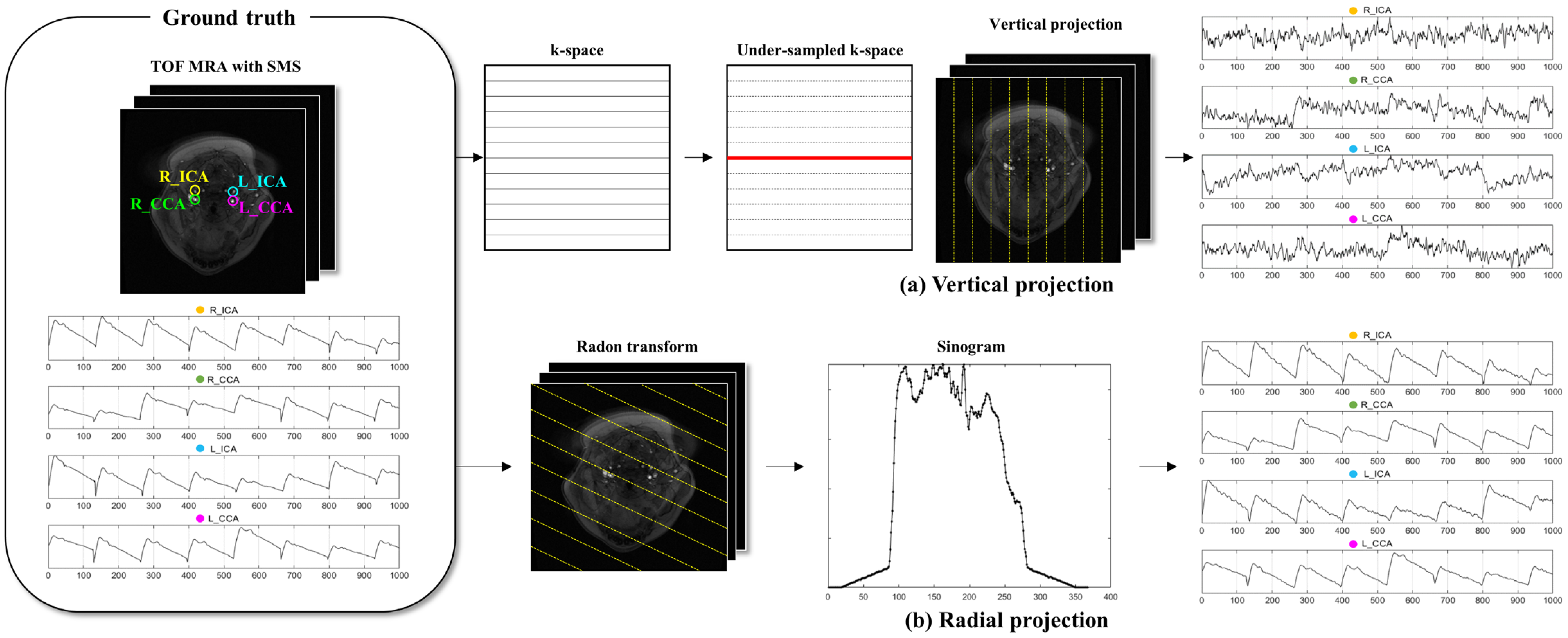
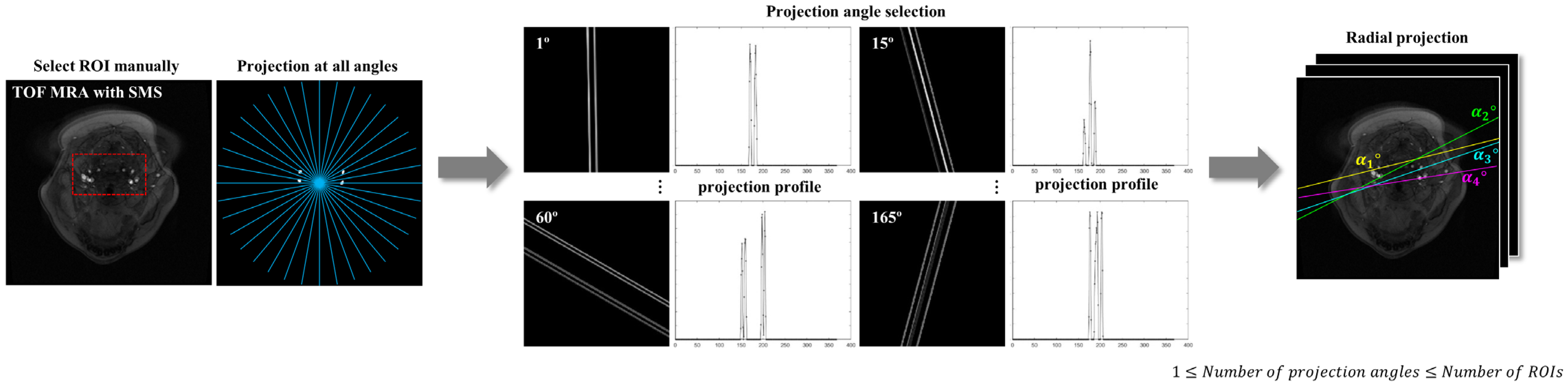
2.2. Projection Methods
2.3. PWV Calculation
2.4. Evaluation with Error Analysis
3. Results
4. Discussion
5. Conclusions
Author Contributions
Funding
Institutional Review Board Statement
Informed Consent Statement
Data Availability Statement
Conflicts of Interest
References
- Cecelja, M.; Chowienczyk, P. Role of Arterial Stiffness in Cardiovascular Disease. JRSM Cardiovasc. Dis. 2012, 1, 1–10. [Google Scholar] [CrossRef] [PubMed]
- Kim, H.-L.; Kim, S.-H. Pulse Wave Velocity in Atherosclerosis. Front. Cardiovasc. Med. 2019, 6, 41. [Google Scholar] [CrossRef] [PubMed]
- Gąsecki, D.; Rojek, A.; Kwarciany, M.; Kowalczyk, K.; Boutouyrie, P.; Nyka, W.; Laurent, S.; Narkiewicz, K. Pulse Wave Velocity Is Associated with Early Clinical Outcome after Ischemic Stroke. Atherosclerosis 2012, 225, 348–352. [Google Scholar] [CrossRef] [PubMed]
- Kim, J.; Cha, M.-J.; Lee, D.H.; Lee, H.S.; Nam, C.M.; Nam, H.S.; Kim, Y.D.; Heo, J.H. The Association between Cerebral Atherosclerosis and Arterial Stiffness in Acute Ischemic Stroke. Atherosclerosis 2011, 219, 887–891. [Google Scholar] [CrossRef] [PubMed]
- Laurent, S.; Katsahian, S.; Fassot, C.; Tropeano, A.-I.; Gautier, I.; Laloux, B.; Boutouyrie, P. Aortic Stiffness Is an Independent Predictor of Fatal Stroke in Essential Hypertension. Stroke 2003, 34, 1203–1206. [Google Scholar] [CrossRef]
- Fiori, G.; Fuiano, F.; Scorza, A.; Conforto, S.; Sciuto, S.A. Non-Invasive Methods for PWV Measurement in Blood Vessel Stiffness Assessment. IEEE Rev. Biomed. Eng. 2022, 15, 169–183. [Google Scholar] [CrossRef]
- Darnaud, C.; Courtet, A.; Schmitt, A.; Boutouyrie, P.; Bouchard, P.; Carra, M.C. Association between Periodontitis and Pulse Wave Velocity: A Systematic Review and Meta-Analysis. Clin. Oral. Investig. 2021, 25, 393–405. [Google Scholar] [CrossRef]
- Wentland, A.L.; Grist, T.M.; Wieben, O. Review of MRI-Based Measurements of Pulse Wave Velocity: A Biomarker of Arterial Stiffness. Cardiovasc. Diagn. Ther. 2014, 4, 193. [Google Scholar]
- Jiang, B.; Liu, B.; McNeill, K.L.; Chowienczyk, P.J. Measurement of Pulse Wave Velocity Using Pulse Wave Doppler Ultrasound: Comparison with Arterial Tonometry. Ultrasound Med. Biol. 2008, 34, 509–512. [Google Scholar] [CrossRef]
- Laurent, S.; Cockcroft, J.; Van Bortel, L.; Boutouyrie, P.; Giannattasio, C.; Hayoz, D.; Pannier, B.; Vlachopoulos, C.; Wilkinson, I.; Struijker-Boudier, H.; et al. Expert Consensus Document on Arterial Stiffness: Methodological Issues and Clinical Applications. Eur. Heart J. 2006, 27, 2588–2605. [Google Scholar] [CrossRef]
- Urban, M.W. Understanding Arterial Biomechanics with Ultrasound and Waveguide Models. Acoust. Today 2023, 19, 46. [Google Scholar] [CrossRef] [PubMed]
- Vappou, J.; Luo, J.; Okajima, K.; Di Tullio, M.; Konofagou, E. Aortic Pulse Wave Velocity Measured by Pulse Wave Imaging (PWI): A Comparison with Applanation Tonometry. Artery Res. 2011, 5, 65–71. [Google Scholar] [CrossRef] [PubMed]
- Bossuyt, J.; Van De Velde, S.; Azermai, M.; Vermeersch, S.J.; De Backer, T.L.M.; Devos, D.G.; Heyse, C.; Filipovsky, J.; Segers, P.; Van Bortel, L.M. Noninvasive Assessment of Carotid-Femoral Pulse Wave Velocity: The Influence of Body Side and Body Contours. J. Hypertens. 2013, 31, 946–951. [Google Scholar] [CrossRef] [PubMed]
- Yi, K.-K.; Park, C.; Yang, J.; Lee, Y.-B.; Kang, C.-K. Quantitative Thermal Stimulation Using Therapeutic Ultrasound to Improve Cerebral Blood Flow and Reduce Vascular Stiffness. Sensors 2023, 23, 8487. [Google Scholar] [CrossRef]
- Graf, S.; Craiem, D.; Barra, J.G.; Armentano, R.L. Estimation of Local Pulse Wave Velocity Using Arterial Diameter Waveforms: Experimental Validation in Sheep. J. Phys. Conf. Ser. 2011, 332, 012010. [Google Scholar] [CrossRef]
- Price, D.J.A. Tissue Doppler Imaging: Current and Potential Clinical Applications. Heart 2000, 84, ii11–ii18. [Google Scholar] [CrossRef]
- Atkinson, P.; Wells, P.N.T. Pulse-Doppler Ultrasound and Its Clinical Application. Yale J. Biol. Med. 1977, 50, 367. [Google Scholar]
- Pilz, N.; Heinz, V.; Ax, T.; Fesseler, L.; Patzak, A.; Bothe, T.L. Pulse Wave Velocity: Methodology, Clinical Applications, and Interplay with Heart Rate Variability. Rev. Cardiovasc. Med. 2024, 25, 266. [Google Scholar] [CrossRef]
- Calabia, J.; Torguet, P.; Garcia, M.; Garcia, I.; Martin, N.; Guasch, B.; Faur, D.; Vallés, M. Doppler Ultrasound in the Measurement of Pulse Wave Velocity: Agreement with the Complior Method. Cardiovasc. Ultrasound 2011, 9, 13. [Google Scholar] [CrossRef]
- Rabben, S.I.; Stergiopulos, N.; Hellevik, L.R.; Smiseth, O.A.; Slørdahl, S.; Urheim, S.; Angelsen, B. An Ultrasound-Based Method for Determining Pulse Wave Velocity in Superficial Arteries. J. Biomech. 2004, 37, 1615–1622. [Google Scholar] [CrossRef]
- Rubens, D.J.; Bhatt, S.; Nedelka, S.; Cullinan, J. Doppler Artifacts and Pitfalls. Radiol. Clin. N. Am. 2006, 44, 805–835. [Google Scholar] [CrossRef] [PubMed]
- Ali, M.F.A. Transcranial Doppler Ultrasonography (Uses, Limitations, and Potentials): A Review Article. Egypt. J. Neurosurg. 2021, 36, 20. [Google Scholar] [CrossRef]
- Purkayastha, S.; Sorond, F. Transcranial Doppler Ultrasound: Technique and Application. Semin. Neurol. 2013, 32, 411–420. [Google Scholar] [CrossRef]
- Geva, T. Magnetic Resonance Imaging: Historical Perspective. J. Cardiovasc. Magn. Reson. 2006, 8, 573–580. [Google Scholar] [CrossRef] [PubMed]
- McDonnell, C.H., 3rd; Herfkens, R.J. Magnetic Resonance Imaging and Measurement of Blood Flow. West. J. Med. 1994, 160, 237. [Google Scholar]
- Barth, M.; Breuer, F.; Koopmans, P.J.; Norris, D.G.; Poser, B.A. Simultaneous Multislice (SMS) Imaging Techniques. Magn. Reson. Med. 2016, 75, 63–81. [Google Scholar] [CrossRef] [PubMed]
- Jung, J.-Y.; Lee, Y.-B.; Kang, C.-K. Novel Technique to Measure Pulse Wave Velocity in Brain Vessels Using a Fast Simultaneous Multi-Slice Excitation Magnetic Resonance Sequence. Sensors 2021, 21, 6352. [Google Scholar] [CrossRef]
- Feng, L. Golden-Angle Radial MRI: Basics, Advances, and Applications. Magn. Reson. Imaging 2022, 56, 45–62. [Google Scholar] [CrossRef]
- Zhu, Y.; Gao, S.; Cheng, L.; Bao, S. Review: K-Space Trajectory Development. In Proceedings of the 2013 IEEE International Conference on Medical Imaging Physics and Engineering, Shenyang, China, 19–20 October 2013; pp. 356–360. [Google Scholar] [CrossRef]
- Berry, E.S.K.; Jezzard, P.; Okell, T.W. The Advantages of Radial Trajectories for Vessel-Selective Dynamic Angiography with Arterial Spin Labeling. Magn. Reson. Mater. Phys. Biol. Med. 2019, 32, 643–653. [Google Scholar] [CrossRef]
- Charlton, P.H.; Harana, J.M.; Vennin, S.; Li, Y.; Chowienczyk, P.; Alastruey, J. Pulse Wave Database (PWDB): A Database of Arterial Pulse Waves Representative of Healthy Adults. Heart Circ. 2019. [Google Scholar] [CrossRef]

| Noise Levels | MAE a Mean ± SD (m/s) | |||
|---|---|---|---|---|
| Radial Projection | Vertical Projection | |||
| Left | Right | Left | Right | |
| 10% | 0.30 ± 0.12 | 0.49 ± 0.28 | 3.95 ± 1.57 | 3.03 ± 1.11 |
| 20% | 0.55 ± 0.32 | 0.74 ± 0.34 | 3.27 ± 0.93 | 3.37 ± 1.22 |
| 30% | 1.09 ± 0.64 | 0.94 ± 0.79 | 3.47 ± 1.33 | 3.00 ± 0.98 |
| 40% | 1.24 ± 0.55 | 1.73 ± 1.10 | 3.62 ± 0.81 | 3.31 ± 1.06 |
| 50% | 1.49 ± 1.00 | 1.60 ± 0.96 | 3.77 ± 1.08 | 3.09 ± 0.87 |
| 60% | 1.26 ± 0.67 | 2.12 ± 1.31 | 3.97 ± 1.43 | 3.58 ± 1.06 |
| 70% | 2.27 ± 1.41 | 2.28 ± 1.38 | 3.38 ± 1.70 | 3.18 ± 0.68 |
| 80% | 2.02 ± 0.97 | 2.07 ± 0.82 | 3.21 ± 1.46 | 3.33 ± 1.27 |
| 90% | 3.10 ± 1.66 | 2.54 ± 1.38 | 3.42 ± 1.16 | 3.22 ± 1.06 |
| 100% | 2.45 ± 1.29 | 2.61 ± 1.21 | 3.64 ± 0.76 | 3.21 ± 1.01 |
| Mean ± SD (m/s) | 1.64 ± 0.80 | 3.40 ± 0.28 | ||
| Noise Levels | H | PWV Mean ± SD (m/s) | p (Corrected) | Pairwise Comparisons (DSCF) p | ||||
|---|---|---|---|---|---|---|---|---|
| G (N = 10) | R (N = 10) | V (N = 10) | G-R | G-V | R-V | |||
| 10% | Lt | 2.74 ± 0.27 | 2.79 ± 0.35 | 1.13 ± 2.56 | 1.000 | 0.993 | 0.102 | 0.087 |
| Rt | 2.76 ± 0.50 | 2.82 ± 0.54 | 0.26 ± 1.33 | 0.016 * | 0.938 | 0.004 * | 0.003 * | |
| 20% | Lt | 2.65 ± 0.25 | 2.76 ± 0.48 | 0.75 ± 2.28 | 0.586 | 0.893 | 0.060 | 0.060 |
| Rt | 2.80 ± 0.50 | 2.92 ± 0.43 | 0.19 ± 0.99 | 0.001 * | 0.493 | <0.001 * | <0.001 * | |
| 30% | Lt | 2.67 ± 0.19 | 3.12 ± 0.77 | 0.24 ± 1.78 | 0.109 | 0.684 | 0.037 * | 0.009 * |
| Rt | 2.74 ± 0.43 | 2.99 ± 0.88 | 0.09 ± 1.01 | 0.001 * | 0.951 | <0.001 * | <0.001 * | |
| 40% | Lt | 2.78 ± 0.28 | 3.28 ± 0.63 | 0.40 ± 1.53 | 0.012 * | 0.219 | 0.007 * | 0.003 * |
| Rt | 2.83 ± 0.43 | 3.01 ± 1.26 | −0.22 ± 1.27 | 0.002 * | 0.493 | <0.001 * | <0.001 * | |
| 50% | Lt | 2.63 ± 0.22 | 3.17 ± 1.32 | −0.46 ± 1.16 | 0.001 * | 0.493 | <0.001 * | <0.001 * |
| Rt | 2.82 ± 0.54 | 2.95 ± 1.29 | −0.22 ± 0.71 | 0.001 * | 0.893 | <0 .001 * | <0.001 * | |
| 60% | Lt | 2.74 ± 0.30 | 2.76 ± 0.72 | −0.19 ± 1.98 | 0.047* | 0.988 | 0.007 * | 0.009 * |
| Rt | 2.86 ± 0.48 | 3.15 ± 1.54 | −0.67 ± 0.83 | 0.001 * | 0.588 | <0.001 * | <0.001 * | |
| 70% | Lt | 2.68 ± 0.25 | 2.93 ± 1.07 | 0.50 ± 1.62 | 0.038 * | 0.540 | 0.007 * | 0.009 * |
| Rt | 2.80 ± 0.43 | 2.25 ± 1.28 | 0.14 ± 0.84 | 0.004 * | 0.951 | <0 .001 * | 0.003 * | |
| 80% | Lt | 2.87 ± 0.59 | 2.69 ± 1.18 | 0.44 ± 1.93 | 0.074 | 0.997 | 0.007 * | 0.018 * |
| Rt | 2.89 ± 0.56 | 2.11 ± 0.97 | −0.14 ± 0.88 | 0.002 * | 0.493 | <0.001 * | 0.002 * | |
| 90% | Lt | 2.71 ± 0.56 | 1.00 ± 1.94 | 0.22 ± 1.13 | 0.003 * | 0.006 * | <0.001 * | 0.220 |
| Rt | 2.77 ± 0.53 | 2.33 ± 2.10 | −0.43 ± 0.98 | 0.022 * | 0.818 | <0.001 * | 0.027 * | |
| 100% | Lt | 2.84 ± 0.31 | 2.50 ± 1.06 | 0.00 ± 1.61 | 0.036 * | 0.730 | 0.007 * | 0.007 * |
| Rt | 2.81 ± 0.42 | 1.01 ± 1.28 | −0.38 ± 0.81 | 0.001 * | 0.006 * | <0.001 * | 0.034 * | |
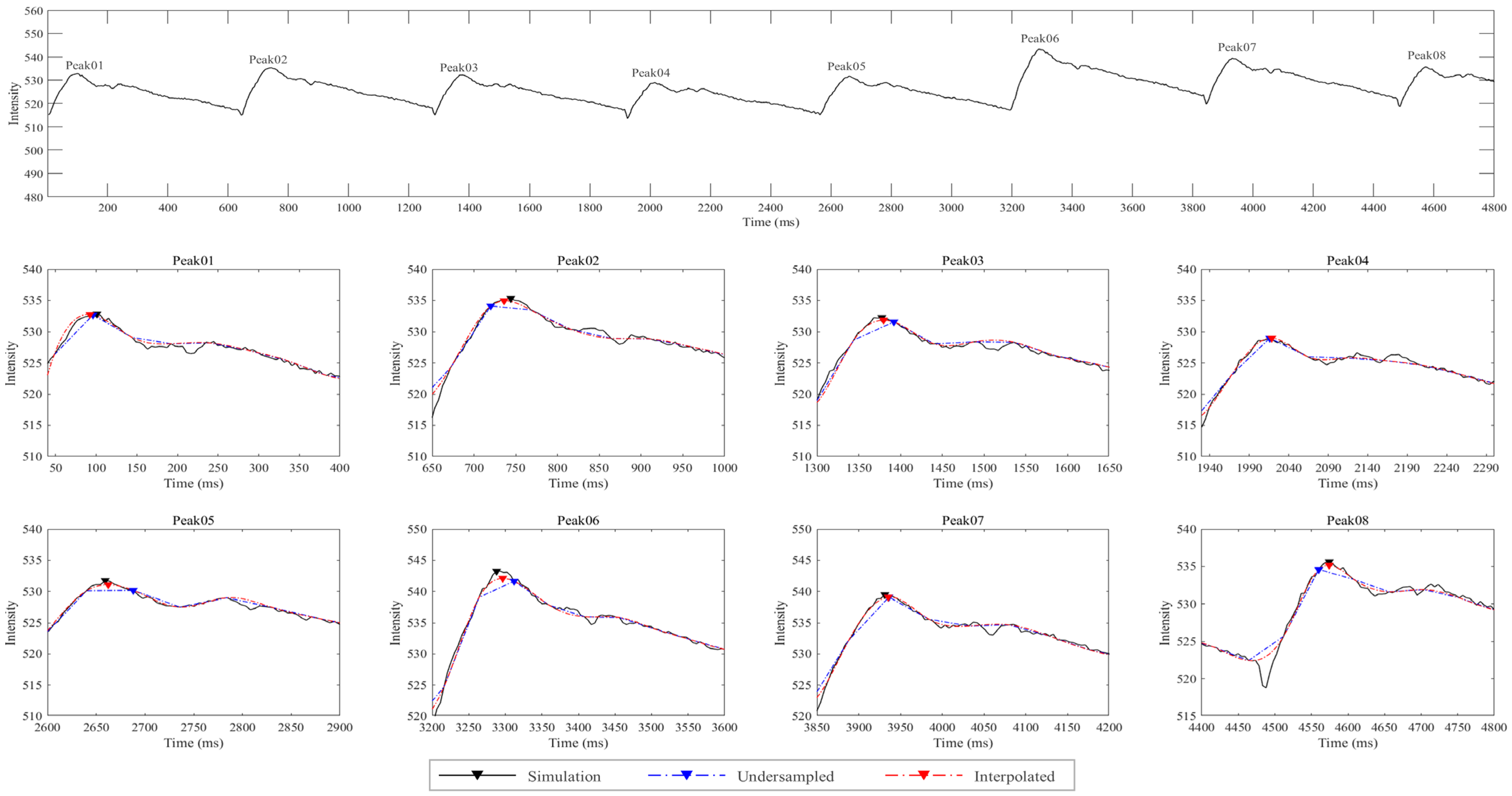
| Noise Levels a | PWV Mean ± SD (m/s) b | p (Corrected) | Pairwise Comparisons (DSCF) p | ||||
|---|---|---|---|---|---|---|---|
| S | U | I | S-U | S-I | U-I | ||
| Without noise | 2.68 ± 0.35 | 1.22 ± 0.07 | 2.87 ± 0.33 | <0.001 * | <0.001 * | 0.052 | <0.001 * |
| 10% | 2.83 ± 0.51 | 1.18 ± 0.14 | 2.86 ± 0.34 | <0.001 * | <0.001 * | 0.679 | <0.001 * |
| 20% | 2.84 ± 0.39 | 1.18 ± 0.14 | 2.83 ± 0.32 | <0.001 * | <0.001 * | 0.960 | <0.001 * |
| 30% | 2.87 ± 0.61 | 1.18 ± 0.14 | 2.86 ± 0.35 | <0.001 * | <0.001 * | 0.366 | <0.001 * |
| 40% | 2.93 ± 0.69 | 1.16 ± 0.16 | 2.86 ± 0.29 | <0.001 * | <0.001 * | 0.902 | <0.001 * |
| 50% | 3.03 ± 0.63 | 1.15 ± 0.18 | 2.90 ± 0.33 | <0.001 * | <0.001 * | 0.958 | <0.001 * |
| 60% | 3.01 ± 0.54 | 1.2 ± 0.14 | 2.88 ± 0.34 | <0.001 * | <0.001 * | 0.944 | <0.001 * |
| 70% | 2.98 ± 0.42 | 1.16 ± 0.10 | 2.81 ± 0.38 | <0.001 * | <0.001 * | 0.689 | <0.001 * |
| 80% | 2.96 ± 0.63 | 1.14 ± 0.20 | 2.85 ± 0.29 | <0.001 * | <0.001 * | 0.996 | <0.001 * |
| 90% | 3.02 ± 0.80 | 1.15 ± 0.18 | 2.92 ± 0.36 | <0.001 * | <0.001 * | 0.645 | <0.001 * |
| 100% | 3.09 ± 0.83 | 1.15 ± 0.30 | 2.88 ± 0.34 | <0.001 * | <0.001 * | 0.890 | <0.001 * |
Disclaimer/Publisher’s Note: The statements, opinions and data contained in all publications are solely those of the individual author(s) and contributor(s) and not of MDPI and/or the editor(s). MDPI and/or the editor(s) disclaim responsibility for any injury to people or property resulting from any ideas, methods, instructions or products referred to in the content. |
© 2025 by the authors. Licensee MDPI, Basel, Switzerland. This article is an open access article distributed under the terms and conditions of the Creative Commons Attribution (CC BY) license (https://creativecommons.org/licenses/by/4.0/).
Share and Cite
Shim, J.-M.; Kang, C.-K.; Son, Y.-D. A Novel Method Combining Radial Projection with Simultaneous Multislice Imaging for Measuring Cerebrovascular Pulse Wave Velocity. Appl. Sci. 2025, 15, 997. https://doi.org/10.3390/app15020997
Shim J-M, Kang C-K, Son Y-D. A Novel Method Combining Radial Projection with Simultaneous Multislice Imaging for Measuring Cerebrovascular Pulse Wave Velocity. Applied Sciences. 2025; 15(2):997. https://doi.org/10.3390/app15020997
Chicago/Turabian StyleShim, Jeong-Min, Chang-Ki Kang, and Young-Don Son. 2025. "A Novel Method Combining Radial Projection with Simultaneous Multislice Imaging for Measuring Cerebrovascular Pulse Wave Velocity" Applied Sciences 15, no. 2: 997. https://doi.org/10.3390/app15020997
APA StyleShim, J.-M., Kang, C.-K., & Son, Y.-D. (2025). A Novel Method Combining Radial Projection with Simultaneous Multislice Imaging for Measuring Cerebrovascular Pulse Wave Velocity. Applied Sciences, 15(2), 997. https://doi.org/10.3390/app15020997