Optimization of Reasonable Finished State for Cable-Stayed Bridge with Steel Box Girder Based on Multiplier Path Following Method

Abstract

The increasing use of cable-stayed bridges with steel box girders necessitates more sophisticated design approaches, as the diverse environments of bridge locations place higher demands on the design process. Determining a reasonable finished state is a critical aspect of bridge design, yet the current methods are significantly constrained. A new approach to optimizing the finished state is proposed. This method’s practicality and efficiency are verified through a case study, analyzing how constraints on vertical girder deflection, horizontal pylon displacement, cable forces, and cable force uniformity affect the optimization outcome. The results show that convergence of the mixed-constraint quadratic programming model is achieved within 30 iterations, yielding an optimized finished state that meets the design criteria. The chosen constraint ranges are deemed appropriate, and the optimization method for the construction stage is thus demonstrably feasible and efficient. The multiplier path following optimization algorithm is computationally efficient, exhibiting good convergence and insensitivity to the problem size. Being easy to program, it avoids the arbitrariness of manual cable adjustment, enabling straightforward determination of a reasonable finished state for the cable-stayed bridge with a steel box girder. The vertical displacement of the main girder, the positive and negative bending moments, and the normal stresses at the top and bottom edges, as well as the positive and negative bending moments in the towers, are significantly influenced by the constraint ranges. The horizontal displacement of the pylon roof is significantly affected by the constraint ranges of both the main girder’s vertical displacement and the pylon’s horizontal displacement, while the remaining constraint ranges have a limited impact.

1. Introduction

A cable-stayed bridge is a composite structural system, primarily composed of cables, pylons, and main girders [1], which has been established it as one of the most competitive bridge types in modern bridge engineering due to its slender and aesthetically pleasing form, combined with its high strength, low self-weight, and significant spanning capacity [2,3]. Cable-stayed bridges with steel box girders, characterized by high structural integrity and efficient construction, are favored by engineers. Recent years have seen increased traffic volumes, leading to the wider application, larger spans, more slender main beams, and greater variety of the structural systems in cable-stayed bridges with steel box girders. Simultaneously, determining a reasonable finished state has become a critical aspect of the design and analytical calculations for cable-stayed bridges [4,5]. Accurate and efficient determination of a reasonable finished state is therefore crucial for the application and development of these bridges.

The design process for cable-stayed bridges with steel box girders aims for a reasonable finished state, characterized by a uniform distribution and a smooth profile of the internal forces in the main girder and pylons under the permanent loads of the erected structure and a uniformly increasing cable force as a function of the cable length. Structural layout and cable forces are the primary factors influencing the reasonable finished state of cable-stayed bridges. Cable forces also influence the structural layout, and adjusting the cable forces is relatively easier. Therefore, cable forces are generally chosen as the optimization objective. During the design of the Swedish Strömsund cable-stayed bridge with steel box girders [6], Dischinger considered cable force calculations for the first time, and cables transitioned from passive load-bearing elements to components capable of actively adjusting the internal force distribution. Optimizing the cable tension allowed for the attainment of reasonable internal forces and profiles in the finished state. This demonstrates that given the structural system and the dead load distribution of a cable-stayed bridge, the problem of optimizing the finished state of a cable-stayed bridge can be transformed into an optimization problem focused on the cable forces [7,8].

Iterative development has led to diverse cable force optimization methods for cable-stayed bridges. The common approaches fall into four categories. The first category comprises optimization methods for specified structural states, primarily including the rigid support continuous beam method [9], the zero-displacement method, and the internal force (stress) equilibrium method [10,11]. While each of these methods has its advantages, they fail to fully account for the stresses and deformations of all of the components in the cable-stayed bridge [12]. The second category employs the minimum bending energy (moment) method [13]. This approach does not target a predetermined structural state but rather optimizes the cable forces by minimizing the structure’s bending strain energy. Notwithstanding capturing the essence of cable force optimization, its capacity is confined to optimizing the cable forces in the dead load state of the completed bridge, excluding considerations of prestress and live loads. The third category utilizes the influence matrix method [14,15]. This approach establishes a functional relationship between the cable forces and optimization objectives through influence matrices. However, relying solely on the influence matrix method does not clearly define the optimization target and often requires a large number of iterations. The fourth category employs mathematical optimization methods [16,17], primarily linear and nonlinear programming algorithms. Linear programming algorithms still fail to account for the states of all of the bridge components. Nonlinear programming algorithms, however, surmount the limitations of the minimum bending energy method, enabling targeted selection of the objective functions, constraints, and optimization algorithms tailored to the specific characteristics of different cable-stayed bridge systems. Nevertheless, the computational process of nonlinear programming algorithms is complex, and controlling the convergence of the results is challenging [18,19]. Accordingly, improving conventional nonlinear programming algorithms is a key path to optimizing the cable forces in cable-stayed bridges.

Advances in technology have significantly aided the optimization of the cable forces in cable-stayed bridges using finite element software, but the underlying logic for solving the problem still relies on nonlinear programming algorithms. Wilson [20] proposed the sequential quadratic programming algorithm in 1963, with significant advancements made by Han and Powell [21,22,23] in the 1970s. Xiao et al. [24] established a mathematical model based on quadratic programming, using the sum of the bending energies of the main beam and pylons as the objective function and incorporating constraints on the longitudinal compression of the main beam, the bending moments in the main beam and pylons, and the support reactions to optimize the cable forces in cable-stayed bridges. Lonetti et al. [25,26] used finite element programs, combined with the allocation principles of dead and live loads, to iteratively define the stresses and cross-sectional properties of post-tensioned stay cables, suspension cables, and main cables, ultimately obtaining the final layout. This procedure also considered the minimum required cross-sectional area of each stay cable under a dead load, verifying the maximum allowable stress and deflection of the cable-stayed bridge under normal and limit states. Hassan et al. [18,27], utilizing the real-coded genetic algorithm (RCGA), employed B-spline interpolation curves to accurately represent the cable force distributions. They effectively addressed the substantial number of variables resulting from the large quantities of cables by calculating the cable forces in steel–concrete composite bridges through minimization of the square root of the sum of the squares (SRSS) of the deflections at the bridge deck and pylon nodes while also minimizing the weight of the steel cables to determine their optimal cross-sectional area. Ha et al. [28] combined a nonlinear, inelastic analysis with genetic algorithms to simultaneously optimize the initial prestress and total weight of the cables using a unit load matrix, significantly reducing the computational costs. Guo et al. [29] combined simulated annealing with cubic B-spline interpolation to select the minimum cable force from the generated objective function values as the optimal solution utilizing the OpenSees platform. The static responses of the deck, pylons, and stay cables in the cable-stayed bridge were then calculated. Sung et al. [30] combined the mutation operations from particle swarm optimization (PSO) and simulated annealing (SA) with the traditional genetic algorithm (GA). By minimizing the deviation between the displacements at completion and the established construction objectives, they enhanced the algorithm’s capacity to escape local minima when calculating the cable forces. Wang et al. [31] employed Midas Civil and MATLAB as their structural analysis and cable force optimization tools, respectively. A multi-objective particle swarm optimization algorithm was used to construct a mathematical model for cable force optimization. Fuzzy set theory was then incorporated to determine the reasonable dead load state of the cable-stayed bridge.

Synthesizing the above, the aforementioned methods have propelled the development of cable force optimization in cable-stayed bridges, but methods optimizing specified structural states fail to address the combined stresses and deformations of all of the bridge components. The minimum bending energy (bending moment) method requires manual cable adjustments to obtain a reasonable force distribution. Using only the influence matrix method results in an ill-defined optimization objective and a large number of iterations. Some mathematical optimization methods have complex calculation processes and may fail to converge if the constraints are not appropriately chosen. To address this, this article innovatively simplifies the optimization of the reasonable finished state of cable-stayed bridges with steel box girders into a mixed-constraint quadratic programming mathematical model, quantifying the optimization target. The derived multiplier path following optimization algorithm is then employed to determine the reasonable finished state. Subsequently, an optimization analysis of the finished state is conducted using the Xiangshan Port cable-stayed bridge with steel box girders as a case study, validating the method’s feasibility and efficiency. The impact of varying constraint ranges on the optimized results was investigated, offering a new approach to determining the reasonable finished state of cable-stayed bridges with steel box girders.

2. Optimization Principles

Based on the structural attributes of cable-stayed bridges with steel box girders, the principles for establishing a reasonable finished state are outlined below:

• The cable forces should lie between the minimum force required by the cable sag considerations and the maximum force allowed by the material’s strength and should increase uniformly with an increasing cable length. Nevertheless, localized variations in the cable force are permissible in regions such as near the pylon, transition piers, or auxiliary piers.
• The internal forces and normal stresses in the main beam should be small and uniformly distributed to ensure that the normal stresses at the top and bottom edges of the cross-section do not exceed the allowable values specified in the code under the most adverse load combinations.
• The eccentricity of the pylon should be minimized to ensure a smaller bending moment in the pylon. Considering live loads and the most adverse load combinations, the pylon should be pre-eccentricated towards the outer span under the dead load of the completed bridge.
• The transition and auxiliary piers should possess an adequate upward vertical reaction capacity under a dead load to minimize the occurrence of negative reactions under a live load. Should negative reactions prove unavoidable, the counterweights or tension-type supports can be incorporated to satisfy the design requirements.

3. The Optimization Model

3.1. Design Variables

In the optimization analysis of a cable-stayed bridge with steel box girders, the cable forces are treated as unknown variables. The entire bridge comprises n fully independent pairs of stay cables. The forces of each stay cable $T_{\mathrm{i}}(i=1,2,\cdots ,n)$, represented vectorially, are as follows:

$$T={\left(T_1,T_2,\cdots ,T_{\mathrm{n}}\right)}^{\mathrm{T}}$$

(1)

3.2. The Optimized Objective

Utilizing the sum of the bending energies of the main beam and the pylon [13] as the optimization objective function, this function provides a comprehensive representation of the overall structural state, leading to satisfactory results for both the displacements and member forces. The objective function can be expressed as

$$U={\displaystyle \underset{\mathrm{g}}{\int }\frac{M^2}{2EI}\mathrm{d}s}+{\displaystyle \underset{\mathrm{p}}{\int }\frac{M^2}{2EI}\mathrm{d}s}$$

(2)

where g represents the main beam, and p represents the pylon.

For discrete beam structures, assuming a constant material elastic modulus $E_{\mathrm{i}}$ and sectional moment of inertia $I_{\mathrm{i}}$ along each element length, the combined bending energy of the steel box girder and pylons can be expressed as

$$U={\displaystyle \sum _{\mathrm{i}=1}^{\mathrm{m}}\frac{L_{\mathrm{i}}}{4E_{\mathrm{i}}{I}_{\mathrm{i}}}}\left(M_{\mathrm{Li}}^2+M_{\mathrm{Ri}}^2\right)$$

(3)

where $m$ represents the total number of main girder and pylon units; $L_{\mathrm{i}}$ represents the length of element $\mathrm{i}$; and $M_{\mathrm{Li}}$ and $M_{\mathrm{Ri}}$ represent the bending moments of the left and right sides of element $\mathrm{i}$, respectively, under a dead load.

Formula (3) can be expressed in matrix form

$$U=M_{\mathrm{L}}^{\mathrm{T}}B{M}_{\mathrm{L}}+M_{\mathrm{R}}^{\mathrm{T}}B{M}_{\mathrm{R}}$$

(4)

where $B=\mathrm{diag}(L_{\mathrm{i}}/4E_{\mathrm{i}}{I}_{\mathrm{i}})(i=1,2,\cdots ,m)$; $M_{\mathrm{L}}$ and $M_{\mathrm{R}}$ represent the bending moment vectors of the left and right sides of the elements, respectively, under a dead load.

The concept of the influence matrix [14] yields

$$\left\{\begin{array}{c}{M}_{\mathrm{L}}=M_{\mathrm{LD}}+C_{\mathrm{ML}}T\\ M_{\mathrm{R}}=M_{\mathrm{RD}}+C_{\mathrm{MR}}T\end{array}\right.$$

(5)

where $M_{\mathrm{LD}}$ and $M_{\mathrm{RD}}$ represents the bending moment vectors of the left and right sides of the elements, respectively, under self-weight and a secondary dead load; $C_{\mathrm{ML}}$ and $C_{\mathrm{MR}}$ represents the influence matrix of the bending moments of the left and right sides of the elements, respectively, under a unit cable force; $T$ represents the cable force vector.

Substituting Formula (5) into Formula (4) yields Formula (6):

$$U=T^{\mathrm{T}}HT+2c^{\mathrm{T}}T+F$$

(6)

where $H=C_{\mathrm{ML}}^{\mathrm{T}}B{C}_{\mathrm{ML}}+C_{\mathrm{MR}}^{\mathrm{T}}B{C}_{\mathrm{MR}}$ is an $n$-order symmetric positive definite matrix, which represents the influence of the unit cable force on the sum of the bending energy of the girder and the pylon; $c^{\mathrm{T}}=M_{\mathrm{LD}}^{\mathrm{T}}B{C}_{\mathrm{ML}}+M_{\mathrm{RD}}^{\mathrm{T}}B{C}_{\mathrm{MR}}$ is an $n$-dimensional column vector, which represents the influence of the self-weight, secondary dead load, and unit cable force on the sum of the bending energy of the girder and the pylon; and $F=M_{\mathrm{LD}}^{\mathrm{T}}B{M}_{\mathrm{LD}}+M_{\mathrm{RD}}^{\mathrm{T}}B{M}_{\mathrm{RD}}$ is a constant which represents the influence of self-weight and the secondary dead load on the sum of the bending energy of the girder and the pylon.

3.3. Constraint Conditions

3.3.1. Constraint on the Cable Force

Cable force constraints are necessary to accommodate the sag and material strength requirements for the cable-stayed bridge under both the dead load condition and operational loading. Based on the influence of structural self-weight and secondary dead loads and employing the concept of influence matrices, these constraints are formulated as

$$T_{\mathrm{L}}\le T_{\mathrm{D}}+C_{\mathrm{T}}T\le T_{\mathrm{U}}$$

(7)

where $T_{\mathrm{U}}$ and $T_{\mathrm{L}}$ represent the specified upper and lower limit values of the cable force, respectively; $T_{\mathrm{D}}$ represents the cable forces generated by self-weight and the secondary dead load; and $C_{\mathrm{T}}$ represents the influence matrix of the cable force under the unit cable force.

3.3.2. A Uniformity Constraint on the Cable Force

With regard to all of the stay cables in cable-stayed bridges, employing only Formula (7) as the constraint for the cable forces may lead to unreasonable differences in the forces between adjacent stay cables. Therefore, it is necessary to incorporate a uniformity constraint on the cable force. This is achieved by introducing a measure of the non-uniformity in the cable forces between adjacent stay cables [32] and constraining this variation to ensure a more uniform distribution. In order to analyze the distribution characteristics of the cable forces within the entire cable-stayed bridge, we introduce the “cable force distribution parameter”. The numerical value of this parameter is directly related to the uniformity of the cable force distribution. If the cable forces of the adjacent three stay cables are denoted as $T_{\mathrm{i}-1}$, $T_{\mathrm{i}}$, and $T_{\mathrm{i}+1}$, then the cable force distribution parameter can be defined as

$$P_{\mathrm{i}}={\displaystyle \frac{T_{\mathrm{i}-1}+T_{\mathrm{i}+1}}{2}}-T_{\mathrm{i}}\hspace{1em}\left(i=2,\cdots ,n-1\right)$$

(8)

And written in matrix form as

$$P=DT$$

(9)

where $D$ is an $(n-2)·n$-order matrix:

$$D={\left[\begin{array}{cccccc}0.5& -1& 0.5& 0& \cdots & 0\\ 0& 0.5& -1& 0.5& \cdots & 0\\ ⋮& ⋮& ⋮& ⋮& \ddots & ⋮\\ 0& 0& 0& 0.5& -1& 0.5\end{array}\right]}_{\left(\mathrm{n}-2,\mathrm{n}\right)}$$

Then, the uniformity constraint on cable forces can be expressed as

$$P_{\mathrm{L}}\le P\le P_{\mathrm{U}}$$

(10)

where $P_{\mathrm{U}}$ and $P_{\mathrm{L}}$ represent the specified upper and lower limit values of the cable force distribution parameter, a reasonable value of which can be determined through trial and error.

3.3.3. The Displacement Constraint on the Main Girder and the Pylons

The displacements of the main girder and pylons in a cable-stayed bridge with steel box girders can be adjusted during construction using a predetermined camber. However, structural deformation directly reflects the design’s rationality, and appropriate displacement constraints lead to more reasonable finished cable forces under dead load conditions. Therefore, the displacements of the main girder and pylons should be constrained. Based on the influence of the structure’s self-weight and the secondary dead load on displacements and using the concept of influence matrices, the displacement constraint on the structures can be expressed as

$${\delta }_{\mathrm{L}}\le {\delta }_{\mathrm{D}}+C_{\mathrm{\delta }}T\le {\delta }_{\mathrm{U}}$$

(11)

where ${\delta }_{\mathrm{U}}$ and ${\delta }_{\mathrm{L}}$ represents the specified upper and lower limit values of displacement, respectively; ${\delta }_{\mathrm{D}}$ represents the displacement of the structure generated by self-weight and the secondary dead load; and $C_{\mathrm{\delta }}$ represents the influence matrix for the nodal displacements under unit cable force.

3.3.4. Normal Stress Constraints on the Main Girder and the Pylons

The normal stresses in the main girder and pylons should be uniformly distributed and should not exceed the allowable values specified in the codes. Based on the influence of self-weight and the secondary dead load on the structural normal stresses and using the concept of influence matrices, the normal stress constraint on the structures can be expressed as

$${\sigma }_{\mathrm{L}}\le {\sigma }_{\mathrm{D}}+C_{\mathrm{\sigma }}T\le {\sigma }_{\mathrm{U}}$$

(12)

where ${\sigma }_{\mathrm{U}}$ and ${\sigma }_{\mathrm{L}}$ represent the specified upper and lower limit values of normal stress, respectively; ${\sigma }_{\mathrm{D}}$ represents the normal stress of the structure generated by self-weight and the secondary dead load; and $C_{\mathrm{\sigma }}$ represents the influence matrix of structural normal stress under the unit cable force.

3.3.5. Other Constraints

In addition to constraining the displacements, normal stresses, and cable forces of the main girder and pylons within certain ranges, specific values for the deformations and internal forces of certain structural elements can be prescribed within those same ranges. This allows for the inclusion of an equality constraint

$$S_{\mathrm{D}}+C_{\mathrm{e}}T=S$$

(13)

where $S_{\mathrm{D}}$ represents the displacement, internal force, or normal stress of the main girder and pylons and the cable force generated by self-weight and the secondary dead load; $C_{\mathrm{e}}$ represents the influence matrix of the displacement, internal force, or normal stress of the main girder and pylons and the cable force under the unit cable force; and $S$ represents the expectations of the displacement, internal force, or normal stress of the main girder and pylons and the cable force.

3.4. Establishment of the Optimization Model

Based on the analysis above, omitting the constant term in Equation (6) allows for the establishment of a quadratic programming model for optimizing the finished state of the cable-stayed bridge with steel box girders. This simplification yields

$$\left\{\begin{array}{c}\min U\left(T\right)={\displaystyle \frac{1}{2}}{T}^{\mathrm{T}}HT+c^{\mathrm{T}}T\hfill \\ \mathrm{s}.\mathrm{t}.\hspace{1em}AT\ge b, C_{\mathrm{e}}T=f\hfill \end{array}\right.$$

(14)

where $A={\left[\begin{array}{cccccccc}{C}_{\mathrm{T}}^{\mathrm{T}}& -C_{\mathrm{T}}^{\mathrm{T}}& D& -D& C_{\mathrm{\delta }}^{\mathrm{T}}& -C_{\mathrm{\delta }}^{\mathrm{T}}& C_{\mathrm{\sigma }}^{\mathrm{T}}& C_{\mathrm{\sigma }}^{\mathrm{T}}\end{array}\right]}^{\mathrm{T}}$ represents an $m\times n$-order matrix, which is the influence matrix of the unit cable forces on the various states of the structure:

$$b={\left[\begin{array}{cccccccc}{\left(T_{\mathrm{L}}-T_{\mathrm{D}}\right)}^{\mathrm{T}}& {\left(-T_{\mathrm{U}}+T_{\mathrm{D}}\right)}^{\mathrm{T}}& P_{\mathrm{U}}& -P_{\mathrm{U}}& {\left({\delta }_{\mathrm{L}}-{\delta }_{\mathrm{D}}\right)}^{\mathrm{T}}& {\left(-{\delta }_{\mathrm{U}}+{\delta }_{\mathrm{D}}\right)}^{\mathrm{T}}& {\left({\sigma }_{\mathrm{L}}-{\sigma }_{\mathrm{D}}\right)}^{\mathrm{T}}& {\left(-{\sigma }_{\mathrm{U}}+{\sigma }_{\mathrm{D}}\right)}^{\mathrm{T}}\end{array}\right]}^{\mathrm{T}}$$

represents an $n$-dimensional column vector, which is the difference between each structural state under self-weight and the secondary dead load and its corresponding upper and lower bounds; $f=S-S_{\mathrm{D}}$ represents an $l$-dimensional column vector, which is the difference between each structural state under self-weight and the secondary dead load and its expected value.

Ultimately, the problem of determining a reasonable finished state of a cable-stayed bridge with steel box girders is reduced into a quadratic programming problem with mixed constraints.

4. Principles and Solving Steps of the Multiplier Path Following Method

4.1. Principles

The multiplier method, an algorithm for solving optimization problems with equality constraints, was proposed by Powell [33] and Hestenes [34] simultaneously and independently in 1969. Its basic principle is that through the introduction of a Lagrange function and an appropriate penalty function, the original problem can be transformed into a series of unconstrained optimization problems. Due to the introduction of the Lagrange function and the appropriate penalty function, this method can surmount the “sick” imperfection in the Lagrange function with an exterior penalty function method.

The path following method, an interior point algorithm for solving linear programming problems, was proposed by Karmarka in 1984. Then, it was developed to solve quadratic programming problems [35]. This algorithm is a polynomial-time algorithm, insensitive to the problem size. Furthermore, the iterations always search within the feasible region towards the optimal solution, exhibiting small computational demands and good convergence. The solution methodology leverages relaxed Karush–Kuhn–Tucker conditions (KKT conditions, necessary and sufficient conditions for the existence of the optimal solution) and the concept of a central path to maintain an approximately optimal search direction in each iteration, thereby transforming the problem of the optimal solution search into a problem of a central path search [36,37,38,39].

To address the mixed-constraint quadratic programming problem presented in Equation (14), this article combines the solution strategies of the two aforementioned methods to develop an improved optimization algorithm: the multiplier path following optimization algorithm. This method’s core idea is as follows: First, the multiplier method is used to transform the mixed-constraint quadratic programming model into a quadratic programming model with only inequality constraints; then, the path following method is employed to solve this modified model, effectively integrating the two algorithms.

4.1.1. Conversion of the Compound Constraints into Inequality Constraints Using the Multiplier Method

For the quadratic programming problem in Formula (14), the augmented Lagrangian function can be defined as follows:

$$\mathrm{\Phi }\left(T,v,\beta \right)=f\left(T\right)-v^{\mathrm{T}}\left(C_{\mathrm{e}}T-f\right)+{\displaystyle \frac{\beta }{2}}{\left(C_{\mathrm{e}}T-f\right)}^{\mathrm{T}}\left(C_{\mathrm{e}}T-f\right)$$

(15)

where $\beta$ represents the penalty parameter; $\nu =(v_1,v_2,\cdots ,v_{\mathrm{l}}{)}^{\mathrm{T}}$ represents the Lagrange multiplier vector, in which $l$ is the number of rows in the coefficient matrix of equality constraint equation $C_{\mathrm{e}}$.

Then, Formula (14) can be converted into

$$\left\{\begin{array}{l}\min \mathrm{\Phi }\left(T,v,\beta \right)\\ \mathrm{s}.\mathrm{t}. AT\ge b\end{array}\right.$$

(16)

4.1.2. Introduction of the Relaxed KKT Condition

According to the KKT conditions of the quadratic programming problem, a sufficient and necessary condition for $T$ to be the optimal solution is the existence of a Lagrange multiplier $y={(y_1,y_2,\cdots ,y_{\mathrm{m}})}^{\mathrm{T}}>0$ and a slack variable $w={(w_1,w_2,\cdots ,w_{\mathrm{m}})}^{\mathrm{T}}>0$ such that

$$\left\{\begin{array}{l}Qx+C-A^{\mathrm{T}}y=0\\ Ax-w-b=0\\ y_{\mathrm{i}}{w}_{\mathrm{i}}=0 \left(i=1,2,\cdots ,m\right)\\ y\ge 0,w\ge 0\end{array}\right.$$

(17)

where ${\mathrm{\nabla }}_{\mathrm{T}}\mathrm{\Phi }={\displaystyle \frac{\partial \mathrm{\Phi }}{\partial T}}$; $Q=H+\beta C_{\mathrm{e}}^{\mathrm{T}}{C}_{\mathrm{e}}$; $C=c-C_{\mathrm{e}}^{\mathrm{T}}\left(v+\beta f\right)$; $m$ is the number of rows in the coefficient matrix of inequality constraint equation $A$.

The relaxed KKT conditions, derived by substituting $YWe=\mu e$ for $y_{\mathrm{i}}{w}_{\mathrm{i}}=0 (i=1,2,\cdots ,m)$, are as follows:

$$\left\{\begin{array}{l}QT+C-A^{\mathrm{T}}y=0\\ AT-w-b=0\\ YWe=\mu e\\ y\ge 0,w\ge 0\end{array}\right.$$

(18)

where $Y=\mathrm{diag}(y_1,y_2,\cdots ,y_{\mathrm{m}})$; $W=\mathrm{diag}(w_1,w_2,\cdots ,w_{\mathrm{m}})$; $e={(1,1,\cdots ,1)}_{\mathrm{m}}^{\mathrm{T}}$; $\mu$ is the center path parameter; and $\mu =\delta {\displaystyle \frac{y^{\mathrm{T}}w}{m}}>0$, $0<\delta <1$.

For each center path parameter $\mu$, Formula (18) has the unique solution $\{T(\mu ),y(\mu ),w(\mu )|\mu >0\}$, named the center path. The path following method attempts to approach the optimal solution gradually through iterating along the direction of the center path.

4.1.3. Solving Along the Direction of the Center Path

The solution with the use of the path following method is as follows: first, arbitrarily choose a point $(T,y,w)$, where $y>0$ and $w>0$; then, determine the direction $(\mathrm{\Delta }T,\mathrm{\Delta }y,\mathrm{\Delta }w)$ such that $(T+\mathrm{\Delta }T,y+\mathrm{\Delta }y,w+\mathrm{\Delta }w)$ satisfies Formula (18), i.e.,

$$\left\{\begin{array}{l}Q\left(T+\mathrm{\Delta }T\right)-A^{\mathrm{T}}\left(y+\mathrm{\Delta }y\right)+C=0\\ A\left(T+\mathrm{\Delta }T\right)-\left(w+\mathrm{\Delta }w\right)-b=0\\ \left(Y+\mathrm{\Delta }Y\right)\left(W+\mathrm{\Delta }W\right)e=\mu e\end{array}\right.$$

(19)

where $\mathrm{\Delta }Y=\mathrm{diag}(\mathrm{\Delta }{y}_1,\mathrm{\Delta }{y}_2,\cdots ,\mathrm{\Delta }{y}_{\mathrm{m}})$; and $\mathrm{\Delta }W=\mathrm{diag}(\mathrm{\Delta }{w}_1,\mathrm{\Delta }{w}_2,\cdots ,\mathrm{\Delta }{w}_{\mathrm{m}})$.

After simplifying the preceding equation and neglecting the second-order incremental terms, the following expression is obtained:

$$-Q\mathrm{\Delta }T+A^{\mathrm{T}}\mathrm{\Delta }y=C+QT-A^{\mathrm{T}}y$$

(20)

$$A\mathrm{\Delta }T-\mathrm{\Delta }w=b-AT+w$$

(21)

$$W\mathrm{\Delta }y+Y\mathrm{\Delta }w=\mu e-YWe$$

(22)

It follows from Formula (22) that

$$\mathrm{\Delta }w=Y^{-1}\left(\mu e-YWe-W\mathrm{\Delta }y\right)$$

(23)

The substitution of Formula (23) into Formula (21), followed by its representation in matrix form, results in the formula below:

$$\left[\begin{array}{cc}-Q& A^{\mathrm{T}}\\ A& Y^{-1}W\end{array}\right]\left[\begin{array}{c}\mathrm{\Delta }T\\ \mathrm{\Delta }y\end{array}\right]=\left[\begin{array}{c}C+QT-A^{\mathrm{T}}y\\ b-AT+\mu Y^{-1}e\end{array}\right]$$

(24)

The solution to Formulas (23) and (24) provides the search direction. A one-dimensional search is then conducted to determine the new solution and the corresponding optimal step length. This iterative procedure is repeated until convergence to a solution meeting the predefined accuracy criterion is achieved.

4.1.4. Determination of the Optimal Step Size

After obtaining the search direction $(\mathrm{\Delta }T,\mathrm{\Delta }y,\mathrm{\Delta }w)$, it is necessary to determine the step size parameter $\lambda$ for movement along this direction to compute the initial value $(T+\lambda \mathrm{\Delta }T,y+\lambda \mathrm{\Delta }y,w+\lambda \mathrm{\Delta }w)$ for the subsequent iteration. However, since $y>0$ and $w>0$, the conditions for the value of $\lambda$ should satisfy

$$\left\{\begin{array}{l}y+\lambda \mathrm{\Delta }y>0\\ w+\lambda \mathrm{\Delta }w>0\end{array}\right.$$

(25)

i.e.,

$$\left\{\begin{array}{l}{y}_{\mathrm{i}}+\lambda \mathrm{\Delta }{y}_{\mathrm{i}}>0\\ w_{\mathrm{i}}+\lambda \mathrm{\Delta }{w}_{\mathrm{i}}>0\end{array}\right.\left(i=1,2,\cdots ,m\right)$$

(26)

Because $y_{\mathrm{i}}>0$, $w_{\mathrm{i}}>0$, $\lambda >0$, it follows that

$$\left\{\begin{array}{l}{\displaystyle \frac{1}{\lambda }}>-{\displaystyle \frac{\mathrm{\Delta }{y}_{\mathrm{i}}}{y_{\mathrm{i}}}}\\ {\displaystyle \frac{1}{\lambda }}>-{\displaystyle \frac{\mathrm{\Delta }{w}_{\mathrm{i}}}{w_{\mathrm{i}}}}\end{array}\right.\left(i=1,2,\cdots ,m\right)$$

(27)

i.e.,

$${\displaystyle \frac{1}{\lambda }}>\underset{i}{\max }\left(-{\displaystyle \frac{\mathrm{\Delta }{y}_{\mathrm{i}}}{y_{\mathrm{i}}}},-{\displaystyle \frac{\mathrm{\Delta }{w}_{\mathrm{i}}}{w_{\mathrm{i}}}}\right)$$

(28)

In order to guarantee the strict satisfaction of Formula (25), we introduce a positive number $p$, which is less than 1 and near 1. Consequently, the step size parameter $\lambda$ is

$$\lambda =\min \left\{p{\left[\underset{\mathrm{i}}{\max }\left(-{\displaystyle \frac{\mathrm{\Delta }{y}_{\mathrm{i}}}{y_{\mathrm{i}}}},-{\displaystyle \frac{\mathrm{\Delta }{w}_{\mathrm{i}}}{w_{\mathrm{i}}}}\right)\right]}^{-1},1\right\}$$

(29)

4.1.5. The Convergence Criterion

During the k-th iteration of the algorithm, we define $\rho =b-A{T}^{(\mathrm{k})}+w^{(\mathrm{k})}$, $\sigma =C+Q{T}^{(\mathrm{k})}-A^{\mathrm{T}}{y}^{(\mathrm{k})}$, and $\gamma =(y^{(\mathrm{k})}{)}^{\mathrm{T}}{w}^{(\mathrm{k})}$, and set the permissible error $\epsilon >0$.

• Condition 1: If $\max (‖\rho ‖,‖\sigma ‖,\gamma ,‖C_{\mathrm{e}}T-f‖)\le \epsilon$, the iteration converges, yielding the optimal solution $T^{*}$ that meets the requirements;
• Condition 2: If $‖C_{\mathrm{e}}T-f‖>\epsilon$ and $‖C_{\mathrm{e}}{x}^{\left(\mathrm{k}\right)}-f‖/‖C_{\mathrm{e}}{T}^{\left(\mathrm{k}+1\right)}-f‖\ge \theta \left(0<\theta <1\right)$, the penalty function ${\beta }^{\left(\mathrm{k}+1\right)}=\alpha {\beta }^{\left(\mathrm{k}\right)}\left(\alpha >1\right)$, and the Lagrange multiplier vector $v$ is updated;
• Condition 3: If $‖C_{\mathrm{e}}T-f‖>\epsilon$ and $‖C_{\mathrm{e}}{x}^{\left(\mathrm{k}\right)}-f‖/‖C_{\mathrm{e}}{T}^{\left(\mathrm{k}+1\right)}-f‖<\theta \left(0<\theta <1\right)$, the penalty function $\beta$ remains unchanged, and the Lagrange multiplier vector $v$ is updated.

The update formula for the Lagrange multiplier vector $v$ is

$$v^{(\mathrm{k}+1)}=v^{\left(\mathrm{k}\right)}-\beta (C_{\mathrm{e}}{T}^{\left(\mathrm{k}\right)}-f)$$

(30)

4.2. Solving Steps

Based on the preceding discussion, the steps for implementing the multiplier path following optimization algorithm to solve the problem are as follows [40]:

• The initialization step involves setting the initial value $T^{\left(1\right)}$, $y^{\left(1\right)}>0$, $w^{\left(1\right)}>0$, $v^{\left(1\right)}>0$, the positive parameter $0<p<1$, $0<\delta <1$, the permissible error $\epsilon >0$, and the iteration counter $k=1$.
• Subsequently, these formulas $\rho =b-A{T}^{\left(\mathrm{k}\right)}+w^{\left(\mathrm{k}\right)}$, $\sigma =C+Q{T}^{\left(\mathrm{k}\right)}-A^{\mathrm{T}}{y}^{\left(\mathrm{k}\right)}$, $\gamma =(y^{\left(\mathrm{k}\right)}{)}^{\mathrm{T}}{w}^{\left(\mathrm{k}\right)}$, and $\mu =\delta {\displaystyle \frac{\gamma }{m}}$ are solved. If the resulting solution satisfies condition $\max (‖\rho ‖,‖\sigma ‖,\gamma ,‖C_{\mathrm{e}}T{w}^{\left(\mathrm{k}\right)}-f‖)\le \epsilon$, we can determine $T^{*}=T^{(\mathrm{k})}$, and the iterative process is terminated. Otherwise, the Lagrange multiplier vector $v$ is updated based on the convergence criterion, and the algorithm proceeds to the next iteration.
• The search direction $(\mathrm{\Delta }{T}^{\left(\mathrm{k}\right)},\mathrm{\Delta }{y}^{\left(\mathrm{k}\right)},\mathrm{\Delta }{w}^{\left(\mathrm{k}\right)})$ is calculated from Formulas (23) and (24).
• The step size parameter $\lambda =\min \{p{[\underset{\mathrm{i}}{\max }(-\mathrm{\Delta }{y}_{\mathrm{i}}^{\left(\mathrm{k}\right)}/y_{\mathrm{i}}^{\left(\mathrm{k}\right)},-\mathrm{\Delta }{w}_{\mathrm{i}}^{\left(\mathrm{k}\right)}/w_{\mathrm{i}}^{\left(\mathrm{k}\right)})]}^{-1},1\}$ is obtained for the search along the direction $(\mathrm{\Delta }{T}^{\left(\mathrm{k}\right)},\mathrm{\Delta }{y}^{\left(\mathrm{k}\right)},\mathrm{\Delta }{w}^{\left(\mathrm{k}\right)})$.
• Following the determination of the step size parameter $\lambda$, these formulas $T^{\left(\mathrm{k}+1\right)}=T^{\left(\mathrm{k}\right)}+\lambda \mathrm{\Delta }{T}^{\left(\mathrm{k}\right)}$, $y^{\left(\mathrm{k}+1\right)}=y^{\left(\mathrm{k}\right)}+\lambda \mathrm{\Delta }{y}^{\left(\mathrm{k}\right)}$, and $w^{\left(\mathrm{k}+1\right)}=w^{\left(\mathrm{k}\right)}+\lambda \mathrm{\Delta }{w}^{\left(\mathrm{k}\right)}$ are solved. Subsequently, the iteration counter k is incremented to k + 1, and the algorithm returns to step 2. Iteration proceeds until convergence is reached [40].

In summary, the iterative application of the multiplier path following optimization algorithm to the stay cable force $T^{(\mathrm{k})}$ aims to obtain the optimal solution $T^{*}$. The iterative process is illustrated in Figure 1 below.

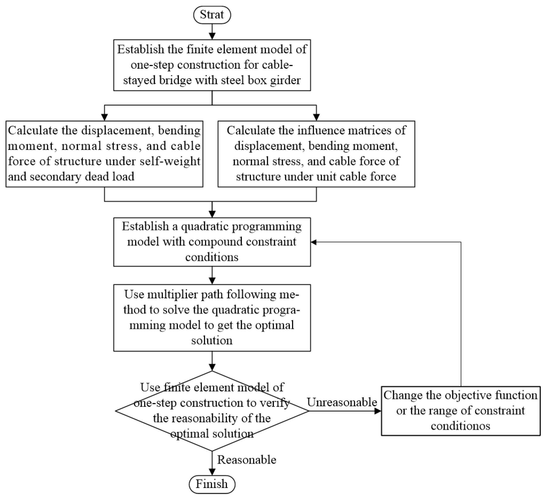
5. The Optimization Method for the Finished State

In light of the foregoing analysis, the optimization process for the finished state of a cable-stayed bridge with steel box girders based on the multiplier path following method can be summarized as follows:

• A finite element analysis is conducted using a model of the cable-stayed bridge with steel box girders that accounts for the finished state. This analysis determines the influence matrices for the displacements, internal forces, normal stresses, and cable forces, as well as these same structural responses under self-weight and secondary dead load conditions.
• The finite element analysis results, in conjunction with Formulas (6) and (14), are used to determine the parameters $H$, $c$, $A$, $b$, and $f$ necessary for the formulation of the quadratic programming model.
• According to the objective function, the constraint conditions, and Formula (14), the quadratic programming model for optimizing the finished state of a cable-stayed bridge can be established.
• Given the initial iterative value $T^{\left(1\right)}$ for the iteration of the initial cable force and the convergence criterion $\epsilon >0$, the MATLAB program [41] is developed based on the multiplier path following optimization algorithm. This program is then used to compute the optimal initial cable force $T^{*}$, satisfying the constraint conditions.
• The reasonableness of $T^{*}$ is assessed by incorporating it into the finite element model and evaluating the results. A reasonable finished state is determined if the computed results satisfy the established constraints; otherwise, iterative refinement involves adjusting the constraint bounds or modifying the objective function, returning to step 3 for model re-optimization and resolution, a process depicted in Figure 2.

6. A Feasibility Analysis of the Optimization Method for the Finished State

6.1. Bridge Overview

The main structure of Xiangshan Port bridge is a five-span, continuous, semi-floating-system cable-stayed bridge with steel box girders, double pylons, and double cable planes, the span arrangement of which is (82 + 262 + 688 + 262 + 82) m, as shown in Figure 3. The pylons employ a diamond-shaped concrete structure, with a total height of 226.5 m, utilizing C50 concrete. The main girder is a flat, streamlined steel box girder, with a standard section width of 26.4 m and a height of 3.5 m at the center line. Q345D steel is employed. The cable stays are composed of parallel high-strength steel wires with a tensile strength of 1670 MPa. A total of 176 cable stays are utilized throughout the bridge, arranged in a double-plane, fan-shaped configuration in space. The main-span cable stays are numbered J1 to J22 from the pylon to the mid-span, and the side-span cable stays are numbered A1 to A22 from the pylon to the transition pier.

6.2. The Finite Element Model

A finite element model of the bridge was developed using the MIDAS Civil 2015 program, employing a “herringbone” calculation scheme. Space frame elements were used to model the main girder, the pylons, and the crossbeam of the pylons, while cable stays were modeled using space truss elements. Rigid arms connected the stay cables to the main girder and towers, as well as the main girder to the crossbeam of the pylons. The pier foundations were modeled as fixed supports, and vertical and horizontal constraints were applied at the appropriate locations on the transition and intermediate piers supporting the main girder.

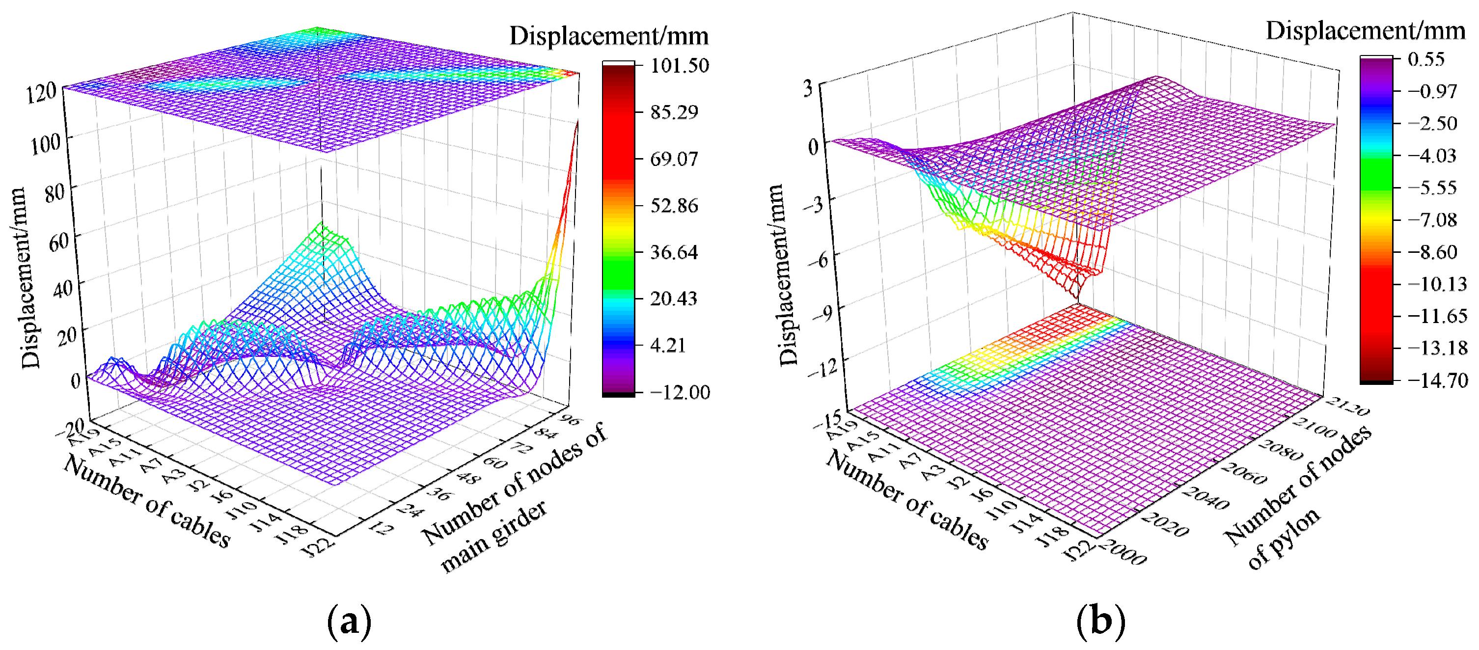
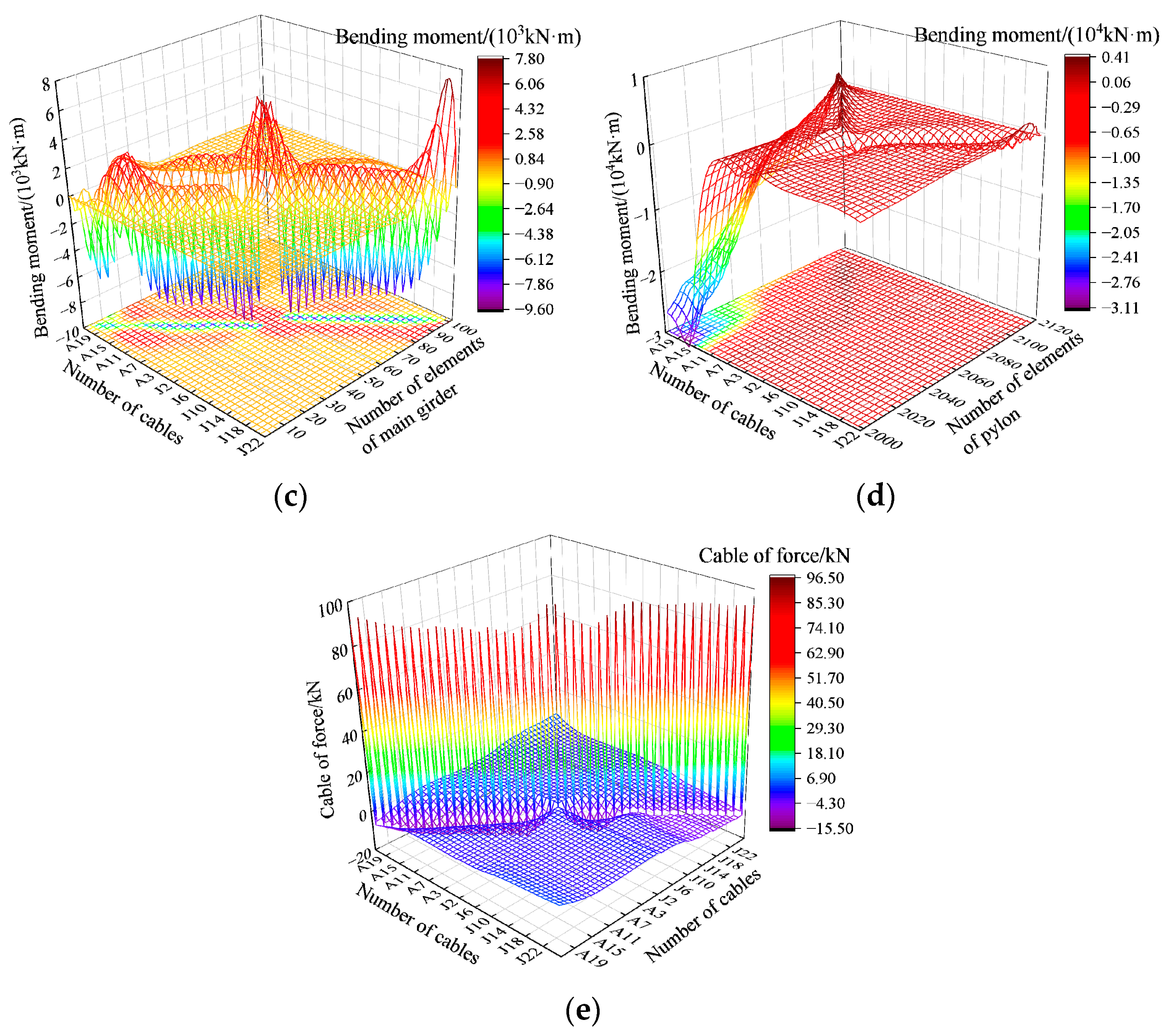
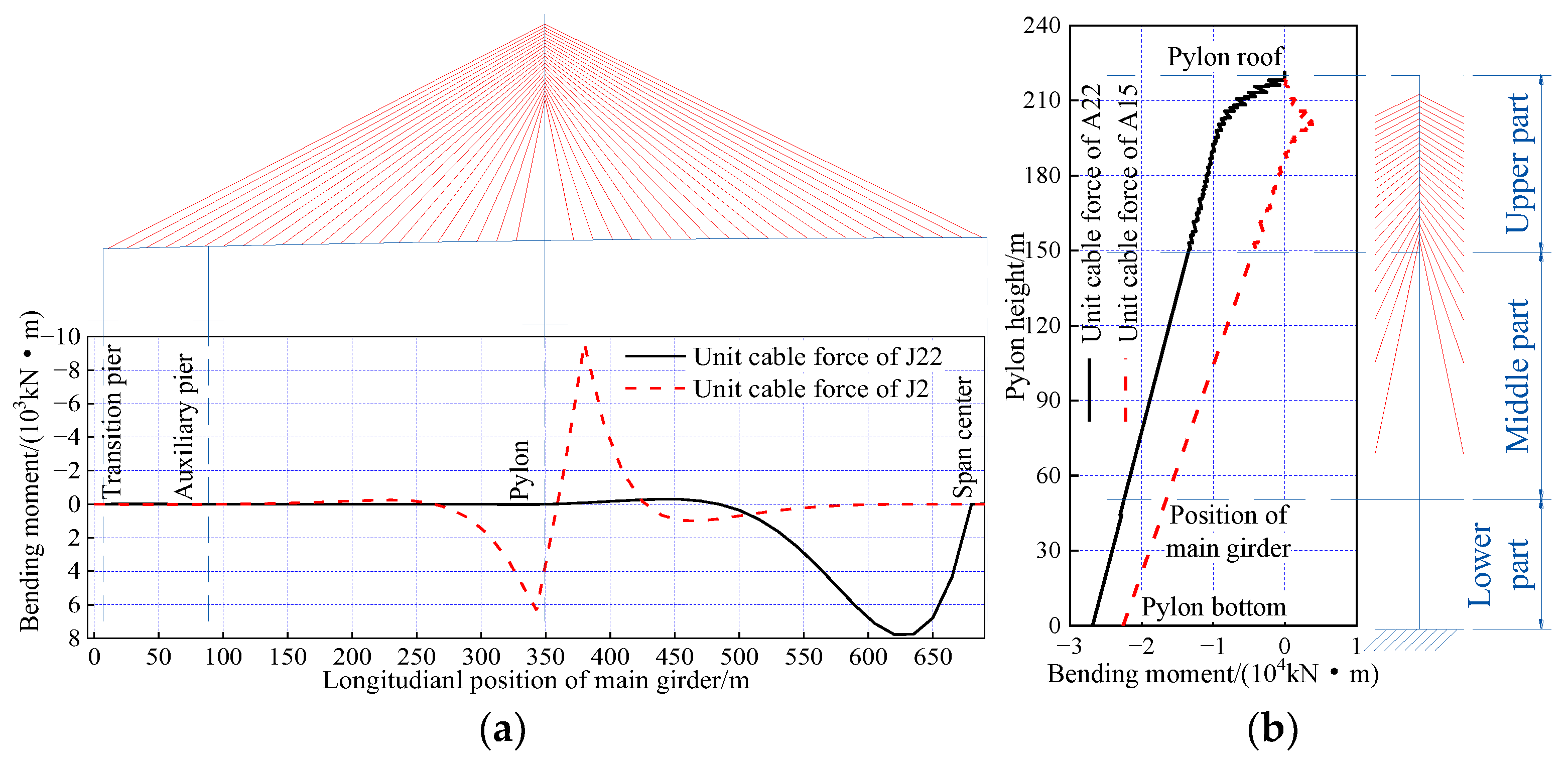
6.3. Calculation of the Influence Matrices

Following the procedure outlined in Figure 2, the influence matrix for the cable forces on the structural displacements, internal forces, and cable forces was first calculated, as shown in Figure 4. This allowed for the determination of the most sensitive cable locations for various states of the main girder and pylons. Due to the symmetrical nature of the bridge in the longitudinal direction, only one half of the structure was considered in the influence matrix calculation. A unit cable force of 1000 kN was employed.

Figure 4a indicates that cable stays J22 and A19 had the greatest influence on the vertical displacement of the main beam. Figure 5 exhibits the maximum influence on the vertical displacement of the main girder. Under a unit cable force of J22 on the main-span side, the maximum upward deflection of the main girder was 101 mm, occurring mid-span. Under a unit cable force of A19 on the side-span side, the maximum downward deflection of the main girder was 12 mm, occurring near $2L/3$ of the adjacent side span. The cable forces of J22 and A22 exhibited the maximum influence on the horizontal displacement of the pylon. Under a unit cable force of J22 on the main-span side, the horizontal displacement of the pylon top was 0.16 mm towards the mid-span side. Under a unit cable force of A22 on the side-span side, the horizontal displacement of the pylon top was 15 mm towards the side-span side.

Figure 4c shows that cable stays J22 and J2 had the greatest influence on the bending moment of the main girder. Figure 6 demonstrates that the cable forces of J22 and J2 had the greatest influence on the bending moment of the main girder. The unit force of cable J22 resulted in a maximum positive bending moment of 7766 kN·m in the main beam, occurring near $2L/5$ of the main span. Under the unit cable force of J2 near the pylon, the maximum negative bending moment of the main girder was −9584 kN·m, occurring at the anchor section of cable J2. The cable forces of A15 and A22 had the greatest influence on the bending moment of the pylon. Under the unit cable force of A15 on the side-span side, the maximum positive bending moment of the pylon was 4042 kN·m, occurring at the upper–middle part of the upper pylon. Under the unit cable force of A22 on the side-span side, the maximum negative bending moment of the pylon was −26,855 kN·m, occurring at the bottom of the pylon.

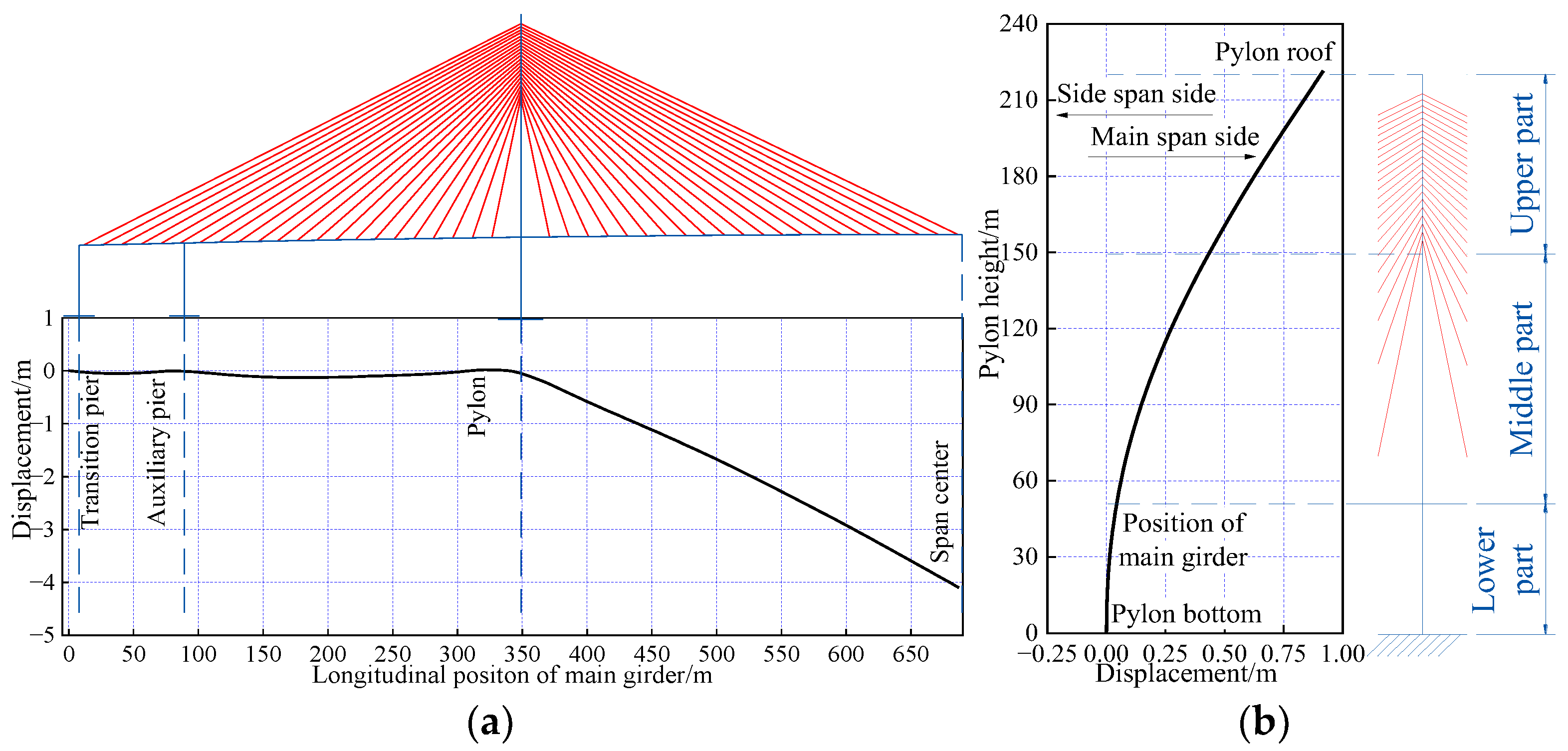
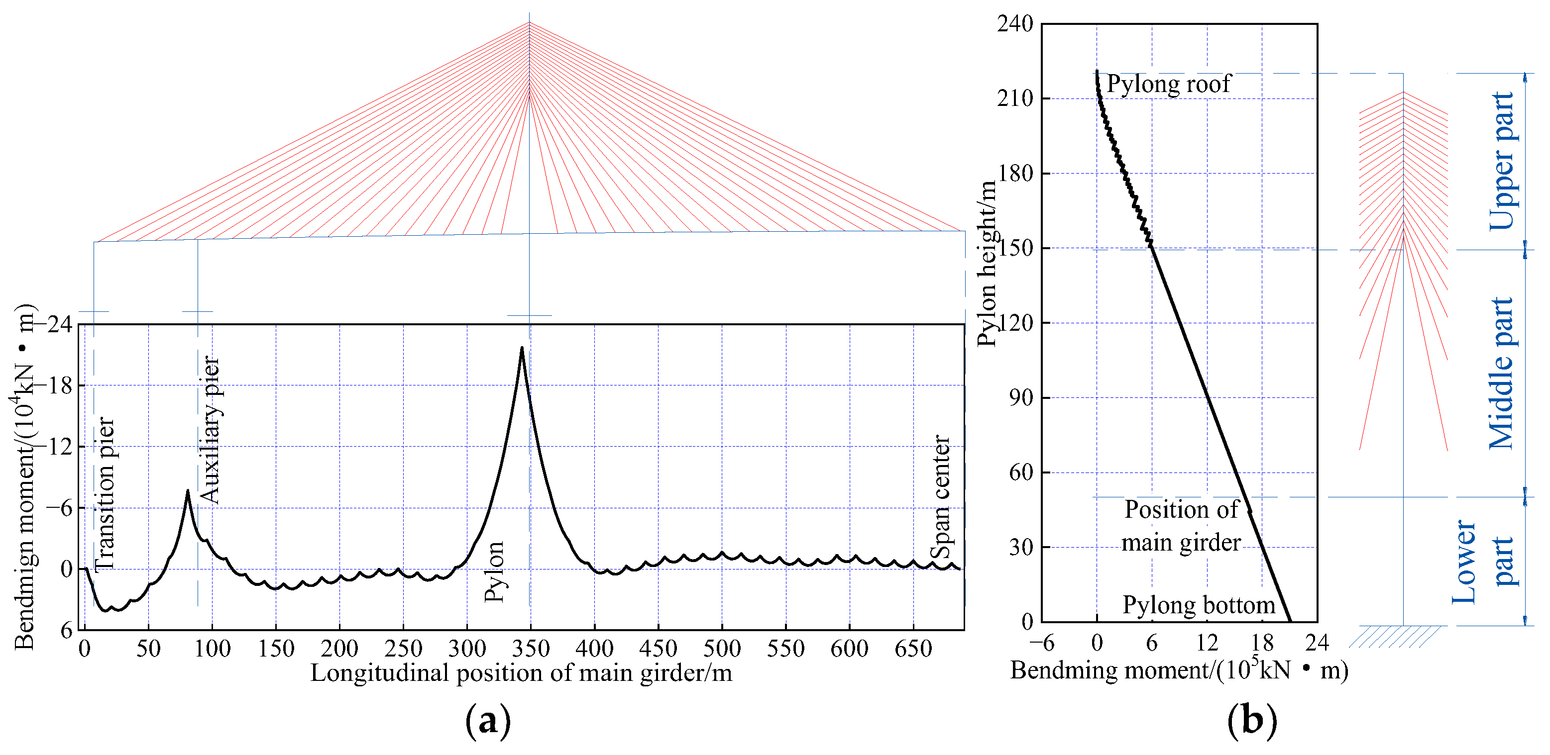
6.4. Calculation of the Structure’s State

As shown in Figure 7, under the action of the self-weight and secondary dead loads (excluding the cable forces), the vertical displacement of the main girder ranged from −4100 mm to 1 mm, with the maximum sag occurring mid-span. The horizontal displacement of the top of the pylon was 918 mm toward the main span.

Figure 8 illustrates the bending moment distributions in the main girder and the pylons under the combined action of self-weight and secondary dead loads (excluding the cable forces). The main girder bending moment ranged from −217,291 to 41,297 kN·m, with the maximum positive moment located approximately at 2L/5 of the side span and the maximum negative moment near the pylon supports. The pylon bending moments ranged from −2,110,609 to 0 kN·m, with the maximum negative moment occurring at the base.

As summarized in Figure 9, the cable forces in the cable-stayed bridge, subjected to self-weight and secondary dead loads (excluding the cable forces), fell within the range of 360 kN to 4026 kN. The maximum cable force was observed in cable J20 located on the mid-span side, whereas the minimum cable force was found in cable J1 near the pylon supports.

6.5. Setting the Optimization Parameters

The determination of reasonable optimization parameters proceeds iteratively. Initially, approximate ranges for each constraint are established empirically. A trial calculation is then performed for a single constraint (e.g., displacement) to refine its acceptable range. This process is repeated for subsequent constraints (e.g., cable tension), holding the previously determined ranges constant. This iterative approach extends to all constraint types. Detailed calculations are presented in Section 7. Based on these trial results, the final optimization parameters are as follows: the cable force $1800 \mathrm{kN}<T_{\mathrm{i}}\le 0.4T_{\mathrm{pdi}}$ ($T_{\mathrm{pdi}}$ is the damage force of cable $i$); the cable force distribution parameter $\left|P_{\mathrm{i}}\right|\le 300 \mathrm{kN}$; the vertical displacement of the main girder nodes $\left|{\delta }_{\mathrm{gi}}\right|\le 150 \mathrm{mm}$; the horizontal displacement of the pylon $-30 \mathrm{mm}\le {\delta }_{\mathrm{pi}}\le 0 \mathrm{mm}$; the normal stresses in the top and bottom flanges of the main girder $\left|{\sigma }_{\mathrm{gi}}\right|\le 120 \mathrm{MPa}$; and the normal stresses on the sides of the pylon ${\sigma }_{\mathrm{pi}}\le 0$.

Through trials, the parameters needed during the optimization process can be set as follow: the initial slack variable vector $w^{\left(1\right)}=(1,\cdots ,1{)}_{\mathrm{m}}^{\mathrm{T}}$; the initial Lagrange multiplier vectors $y^{\left(1\right)}=(1,\cdots ,1{)}_{\mathrm{m}}^{\mathrm{T}}$ and $v^{\left(1\right)}=(1,\cdots ,1{)}_1^{\mathrm{T}}$; the initial iterative cable force vector $T^{\left(1\right)}=(1000,\cdots ,1000{)}_{\mathrm{n}}^{\mathrm{T}}$; and $p=0.95$, $\delta =0.30$, $\alpha =4.00$, ${\beta }^{\left(1\right)}=2.00$, $\theta =0.80$, and the convergence criterion $\epsilon =0.001$.

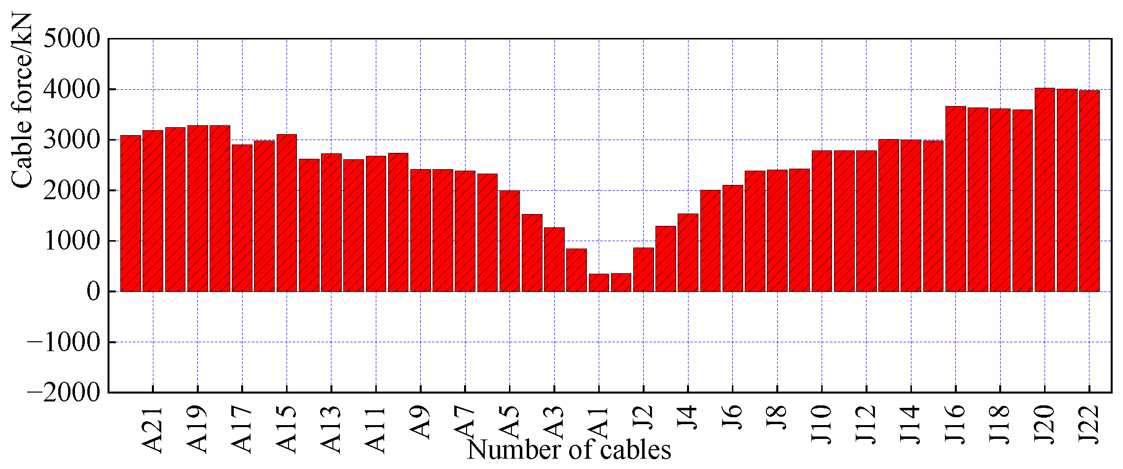
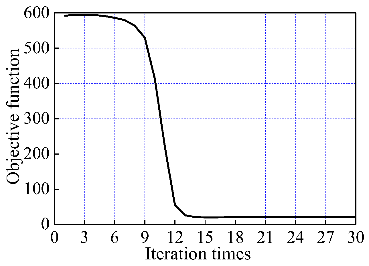
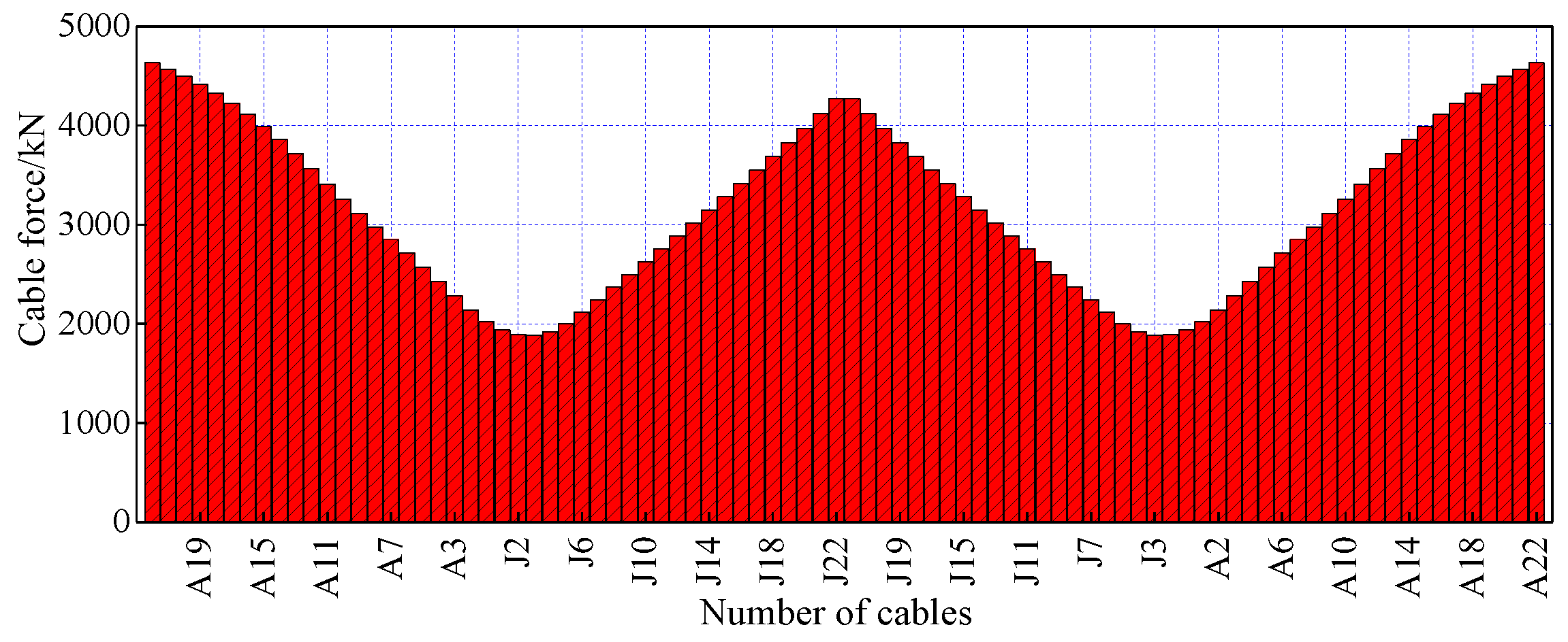
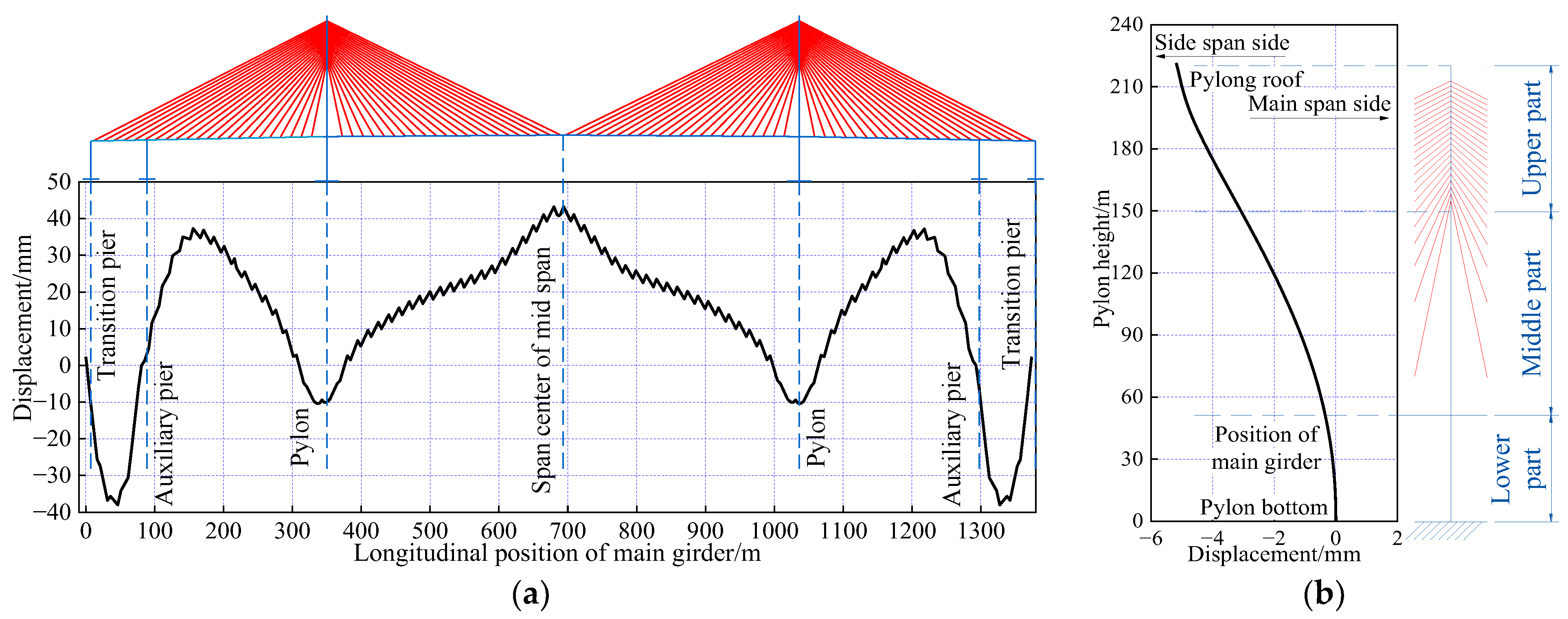
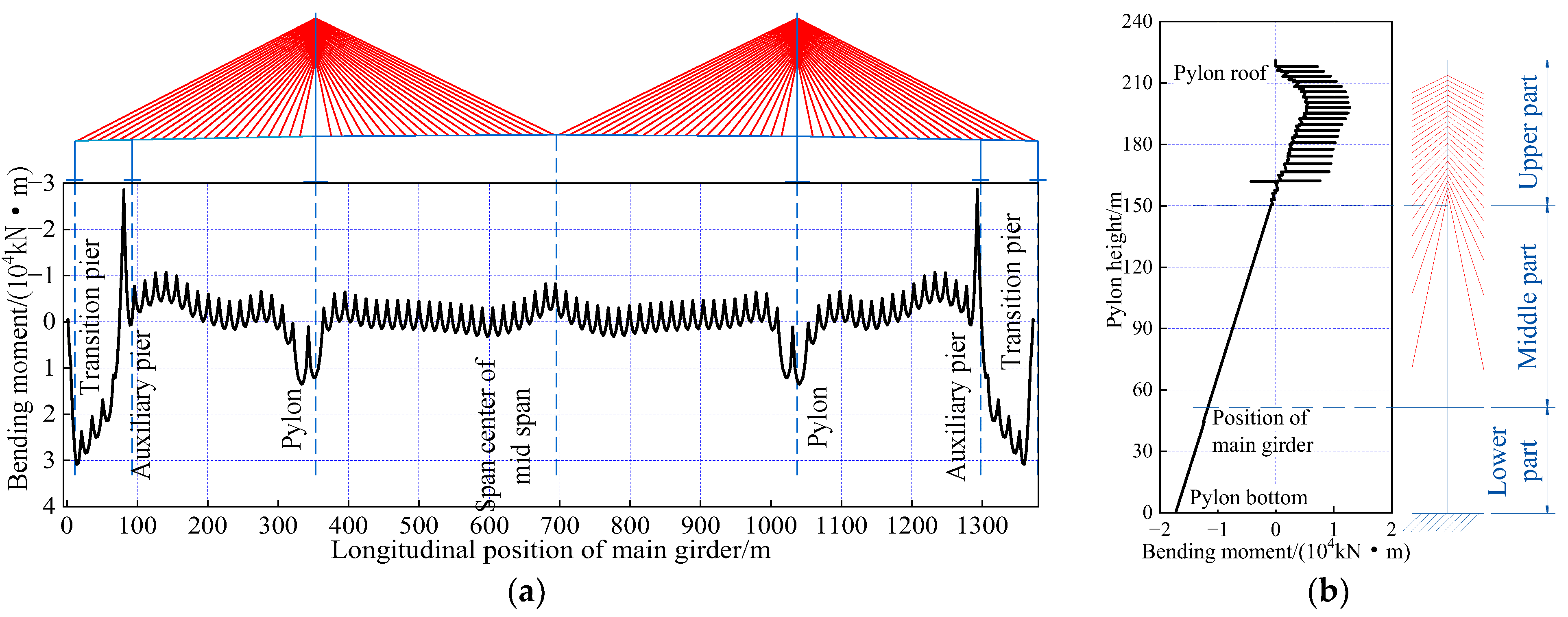
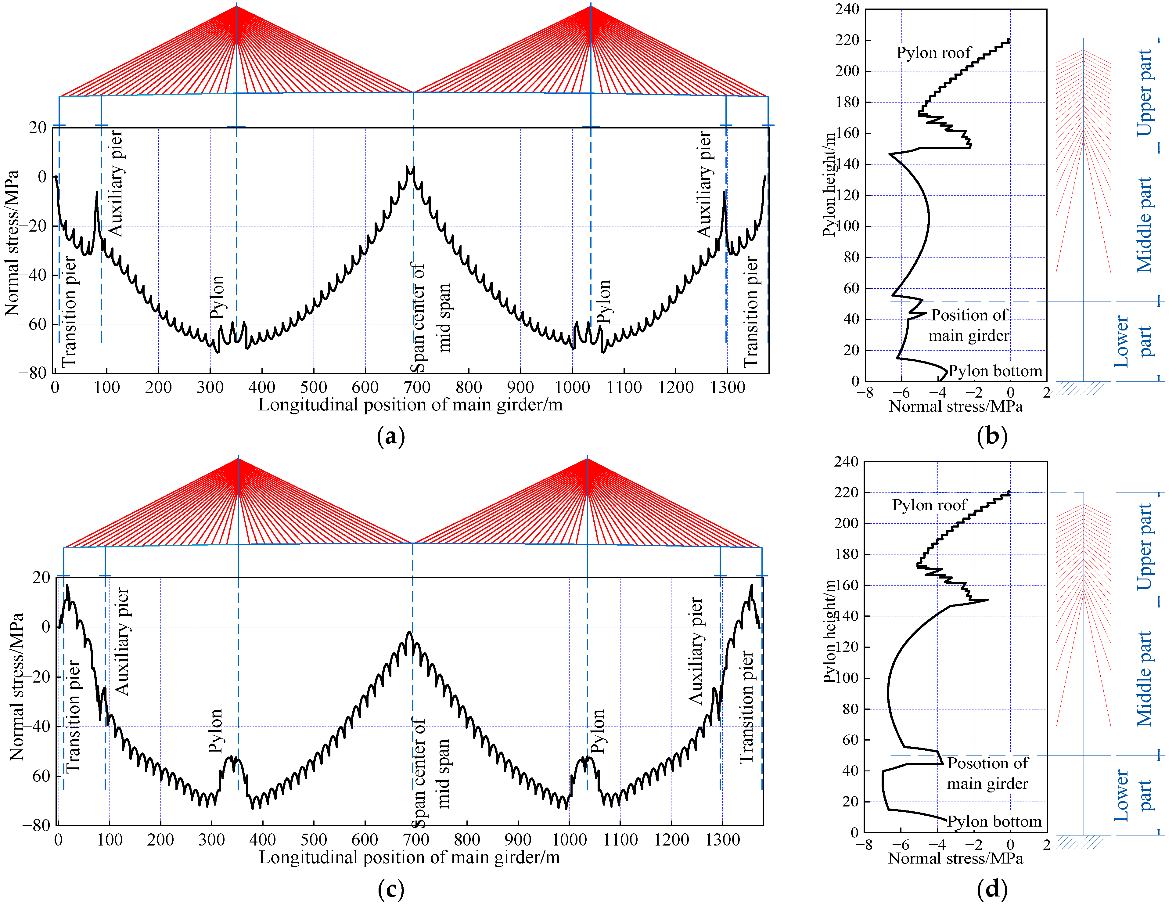
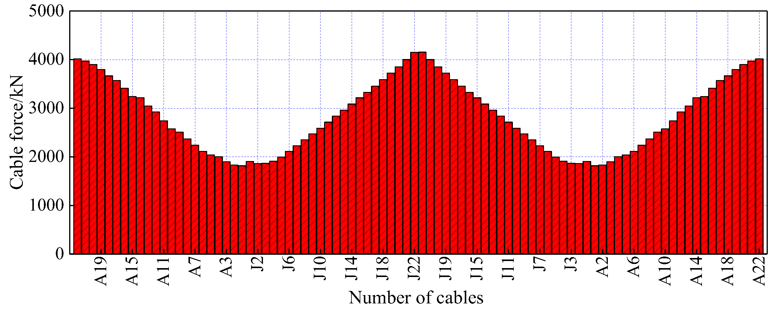
6.6. Optimization Results

The objective function values for the optimization process, as plotted in Figure 10, demonstrate a significant decrease with an increasing number of iterations. Specifically, after 30 iterations, the objective function value dropped from an initial value of 592 to a final value of 21. At this point, $\max (‖\rho ‖,‖\sigma ‖,\gamma ,‖C_{\mathrm{e}}{T}^{\left(\mathrm{k}\right)}-f‖)=4.10\times {10}^{-4}<\epsilon$, which meant that iteration had converged. Thereafter, the optimal cable force sequence, shown in Figure 11, ranged from 1883 kN to 4631 kN. The maximum force occurred in cable A22 on the side span, while the minimum was in cable J3 near the pylon. This sequence was input into a finite element model of the complete bridge (including self-weight, the secondary dead load, the optimal cable forces, and all constraints, without considering the construction stages) to validate the optimization’s accuracy. If the results are reasonable (the evaluation method is referenced in the Optimization Principles section), the optimization of the finished state of the cable-stayed bridge with steel box girders is complete. Otherwise, the constraints or the objective function can be modified to reformulate the quadratic programming model for further optimization.

Figure 12 depicts the distributions of the main girder’s vertical displacement and the pylon’s horizontal displacement under the finished dead load condition. Optimization of the main beam results in vertical displacements ranging from −38 to +43 mm. The maximum positive deflection occurs mid-span, while the maximum negative deflection consistently occurs at the mid-span of the side span. The lateral displacement of the top of the tower is 5 mm towards the side span.

The axial force distributions of the main girder and the pylons under the finished dead load state are shown in Figure 13. The optimized axial forces in the main beam and the pylons are predominantly compressive. The axial force in the main beam ranges from −93,986 to 15 kN and increases uniformly from the transition piers to the pylon. The pylon axial force ranges from −625,872 to −1810 kN and increases uniformly from the top to the bottom of the pylon.

Figure 14 shows the bending moment distributions in the main girder and pylons under the finished dead load condition. Optimization resulted in main girder bending moments ranging from −28,623 to 30,868 kN·m. The maximum positive bending moments occurred near the L/6 point of the side spans, and the maximum negative bending moment occurred at the auxiliary pier’s cap beam sections. The pylon bending moments ranged from −17,291 to 12,765 kN·m, with the largest positive moment at the mid-height of the upper pylon columns and the largest negative moment at the pylon base.

The normal stress of the main girder and pylons under the finished dead load condition is shown in Figure 15. The optimized main beam exhibited a top-surface stress ranging from −71.47 to +4.28 MPa. The maximum compressive stress was observed near the pylon, and the maximum tensile stress occurred mid-span. The bottom flange stresses varied from −73.35 to 17.00 MPa, with the maximum compression near the pylon and the maximum tension near the side spans. For the pylon side-span stresses, the range was −6.67 to −0.01 MPa, exhibiting the maximum compression near the upper pylon connection. The main span’s normal stresses fell between −7.00 and −0.01 MPa, with the maximum compressive stress in the mid–upper portion of the lower pylon columns.

The cable forces under the finished dead load condition are shown in Figure 16. The optimized cable forces increased from the location near the pylon to the transition pier on both sides and were in the range of 4154~1816 kN. The maximum cable force was located in cable J22 on the mid-span side; the minimum cable force was located in cable A1 near the pylon; and the maximum cable force distribution parameter was 153 kN.

The multiplier path following optimization yielded positive vertical support reactions at both the transition and auxiliary piers, indicating an adequate pressure reserve. The vertical support reactions ranged from 4153 to 9762 kN. The maximum vertical reaction was observed at the auxiliary piers, while the minimum was observed at the transition piers.

The above analysis demonstrates that the multiplier path following method, applied to optimizing the finished state of the Xiangshan Port highway bridge, yielded convergence of the objective function within 30 iterations. At this stage, the optimized profile of the main girder is smooth, with a uniform stress distribution along the top and bottom flanges; the top of the pylon exhibits a predetermined lateral offset towards the side span, with a fully compressed cross-section; the cable forces increase uniformly with the cable length; and positive vertical support reactions are observed at both the transition and auxiliary piers, indicating sufficient pressure reserves. This suggests the reasonableness of the constraint range and the feasibility and efficiency of the optimization method for the finished state.

7. The Influence of the Constraint Range on the Optimization Results

This section provides a description of the optimization parameter setting process and an analysis of the sensitivity of the constraint ranges during optimization. The Xiangshan Port bridge is examined using the sum of the bending energies of the girder and the pylon as the objective function. Notably, preliminary calculations indicate that the displacement and cable force constraints exhibit higher sensitivity, while the allowable stress range in the steel box girder is comparatively large, rendering the structural response insensitive to it. Therefore, this section employs the multiplier path following optimization algorithm to optimize the finished state of the cable-stayed bridge, using the constraint on the main girder’s vertical displacement, the constraint on the horizontal displacement of the pylon, the constraint on the stay cable force, and the constraint on the cable force distribution parameter as the variables. This analysis investigates the influence of the constraint ranges on the optimization results. The finite element model and the parameter values used in this optimization process are consistent with those presented in Section 5.

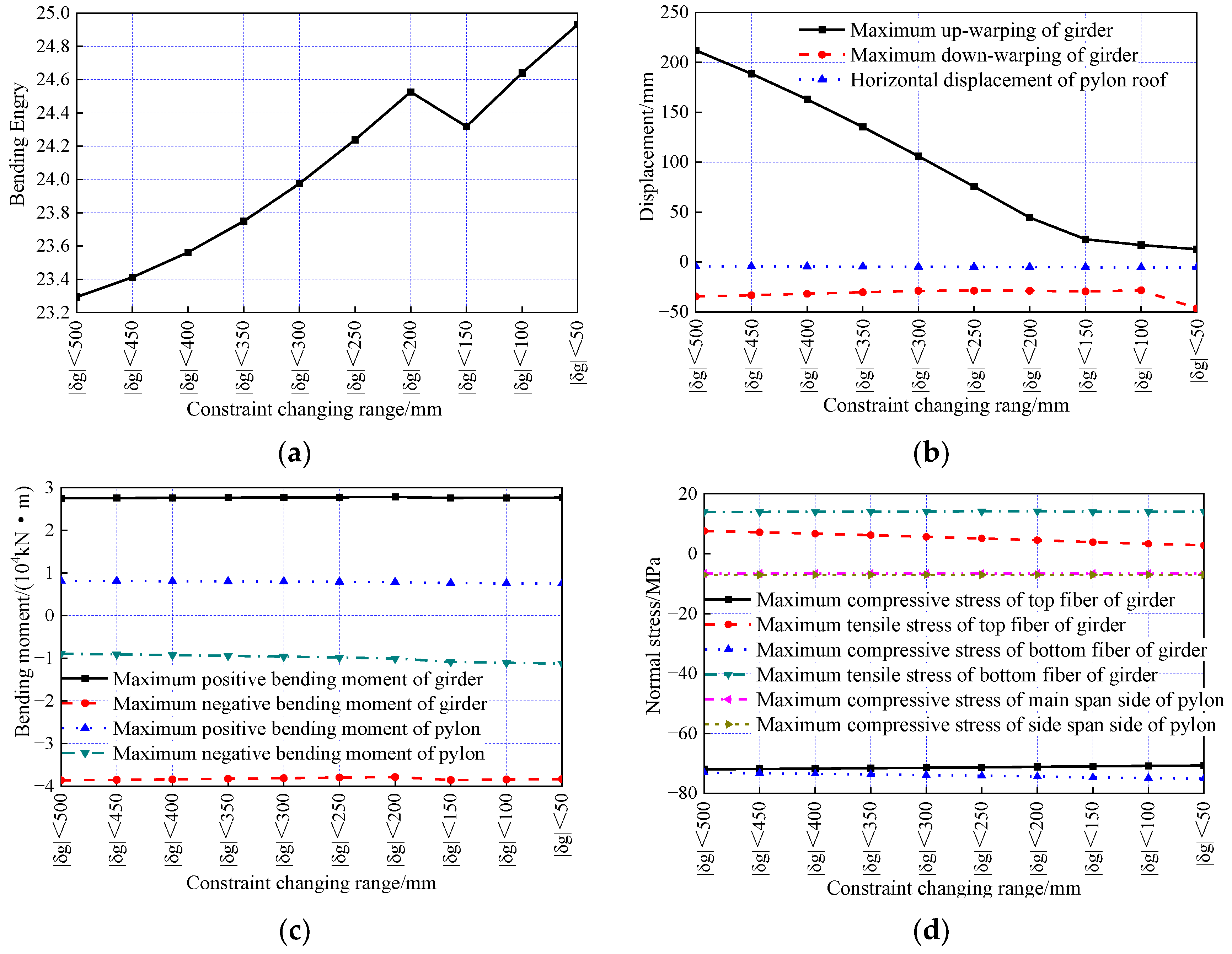
7.1. The Influence of the Constraint Range for the Main Girder’s Vertical Displacement on the Optimization Results

Holding the other constraints constant, the constraint range for the main girder’s vertical displacement was varied from $\left|{\delta }_{\mathrm{g}\mathrm{i}}\right|\le 500 \mathrm{mm}$ to $\left|{\delta }_{\mathrm{g}\mathrm{i}}\right|\le 50 \mathrm{mm}$ to assess its influence on the optimization results. Figure 17 depicts the variations in the structural states corresponding to decreasing the constraint ranges for the main girder’s vertical displacement. Variations in the constraint range for the main girder’s vertical displacement significantly affect the vertical displacement of the main girder, the maximum tensile stress in the main girder top chord, the horizontal displacement of the top of the pylon in the bridge, and the maximum positive and negative bending moments in the bridge pylon. The changes in the other structural states are less than 5%. The maximum vertical deflection of the main girder and the horizontal displacement of the top of the pylon in the bridge both increase as the constraint range for the main girder’s vertical displacement decreases. Conversely, the maximum upward deflection of the main girder, the maximum tensile stress in the main girder’s top chord, and the maximum positive and negative bending moments in the bridge pylon all decrease with a narrowing constraint range. Upon comparing the various results, a constraint on the main girder’s vertical displacement of $\left|{\delta }_{\mathrm{g}\mathrm{i}}\right|\le 150 \mathrm{mm}$ leads to smoother structural alignment and lower maximum positive and negative bending moments in both the main girder and bridge pylons, as well as reduced cable force distribution parameters. Consequently, this constraint range is deemed appropriate.

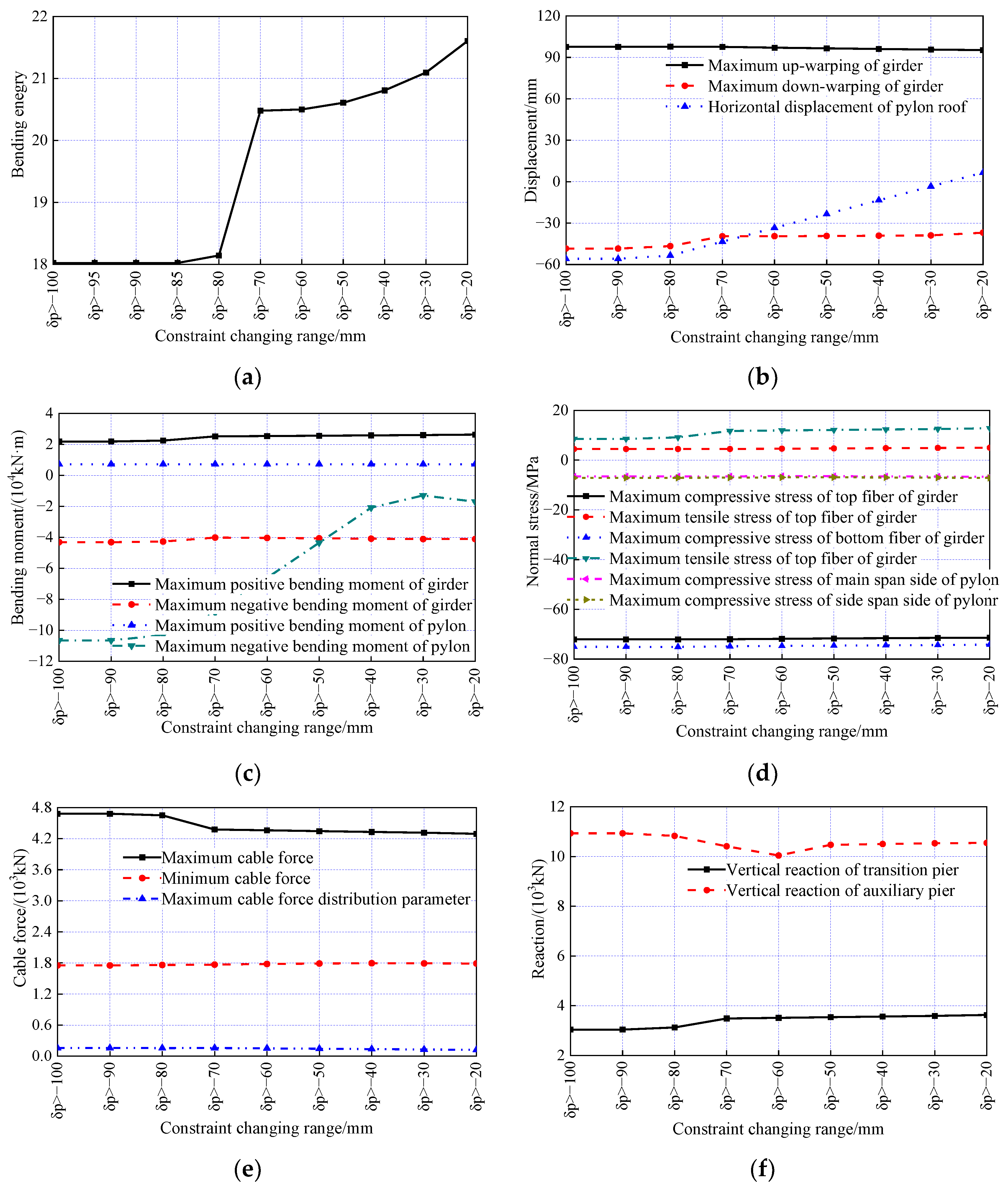
7.2. Influence of a Changing Range of Horizontal Displacements of the Pylon on the Optimization Results

The impact of varying the constraint on the pylon’s horizontal displacement from $-100 \mathrm{mm}\le {\delta }_{\mathrm{pi}}\le 0 \mathrm{mm}$ to $-20 \mathrm{mm}\le {\delta }_{\mathrm{pi}}\le 0 \mathrm{mm}$ while holding the other constraints constant was investigated to assess its effect on the optimization results. The variation in the structural states resulting from changes in the vertical range of constraints on the pylon’s horizontal displacement is presented in Figure 18. Variations in the horizontal pylon displacement constraint range significantly affect the maximum sag of the main girder, the maximum positive and negative bending moments in the main girder, the maximum tensile stress in the top and bottom chords of the main girder, the horizontal displacement of the top of the pylon, the maximum negative bending moment in the pylon, the maximum cable force and cable force distribution parameters, and the vertical reactions of the transition and auxiliary piers. The influence on the other structural states is less than 5%. As the range of the constraints on the pylon’s horizontal displacement narrows, the maximum positive bending moment in the main girder, the maximum tensile stresses in the top and bottom chords of the main girder, and the vertical reaction of the transition pier show an increasing trend. In contrast, the maximum downward deflection of the main girder, the horizontal displacement of the top of the pylon, the maximum cable force, and the cable force distribution parameter decrease. The maximum negative bending moment in the main girder, the maximum negative bending moment in the pylon, and the vertical reaction of the auxiliary pier display non-monotonic behavior, decreasing initially before increasing, with a narrower constraint range. A comparative analysis indicates that a constraint on the pylon’s horizontal displacement of $-30 \mathrm{mm}\le {\delta }_{\mathrm{pi}}\le 0 \mathrm{mm}$ results in smoother structural alignment, lower maximum positive and negative bending moments in the main girder and the pylon, and a reduced maximum cable force distribution parameter. Therefore, this constraint range is considered appropriate.

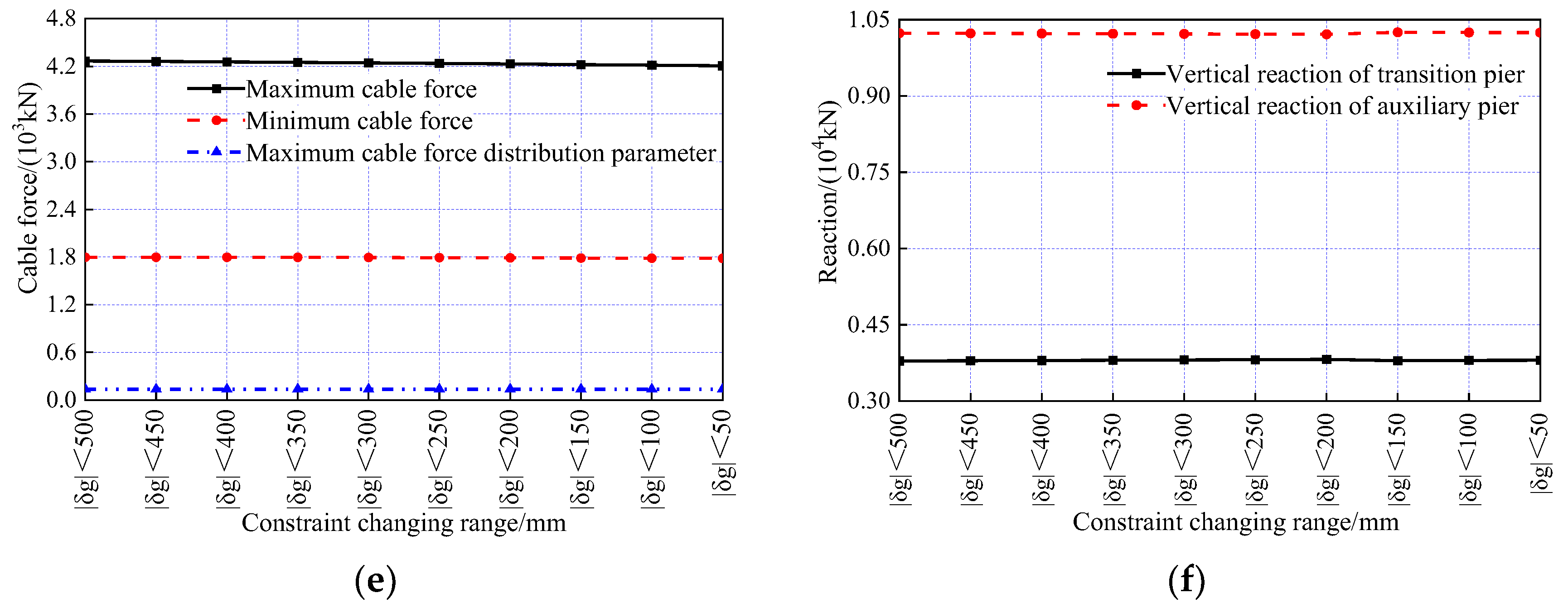
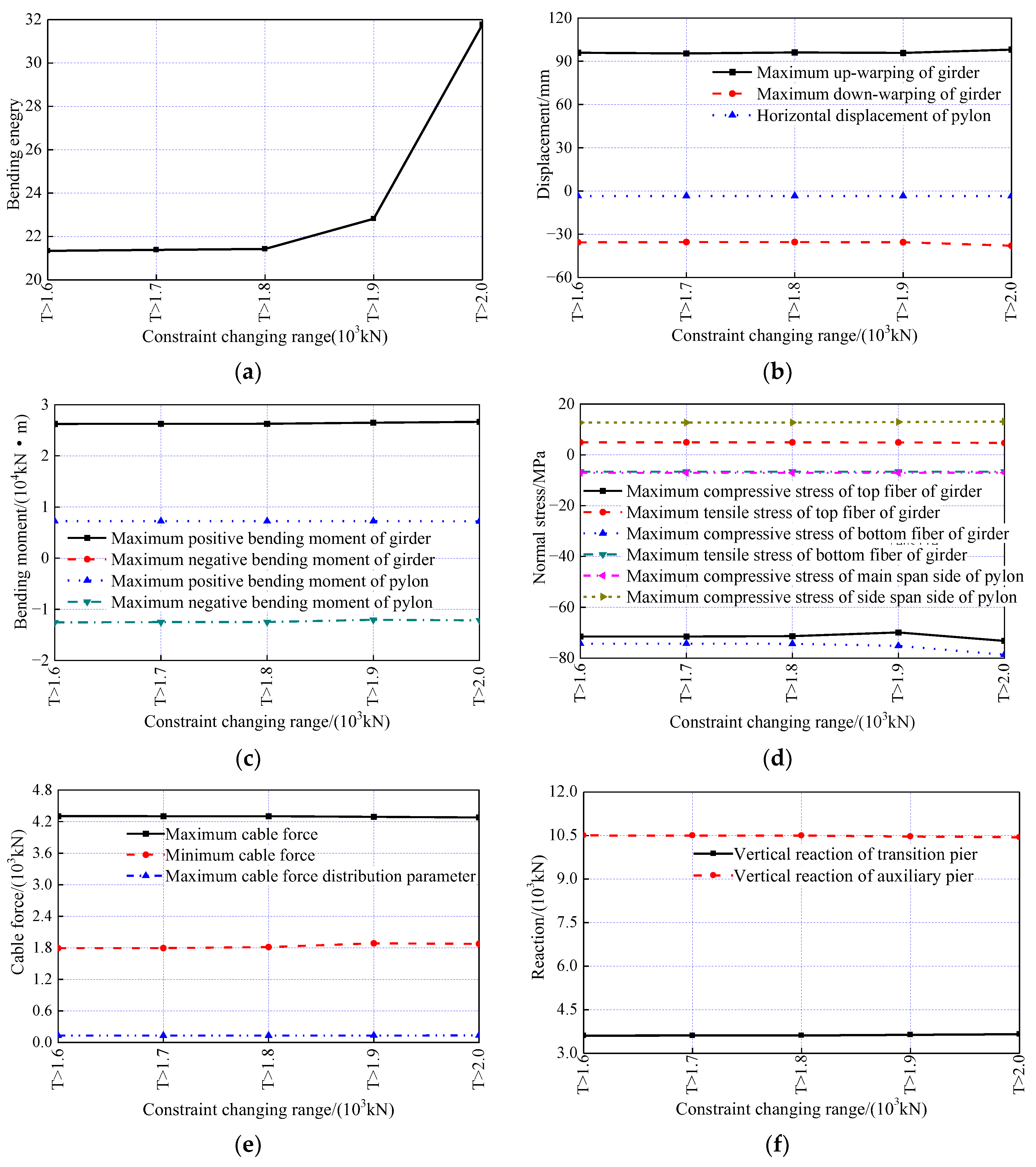
7.3. Influence of the Constraint Range for the Cable Force on the Optimization Results

Maintaining all of the other constraints, the influence of varying the cable force constraint from $1600 \mathrm{kN}\le T_{\mathrm{i}}\le 0.4T_{\mathrm{pdi}}$ to $2000 \mathrm{kN}\le T_{\mathrm{i}}\le 0.4T_{\mathrm{pdi}}$ on the optimization outcomes is examined. Figure 19 illustrates the variations in the structural states as the cable force constraint range is reduced. Changes in the cable force constraint range significantly impact the maximum sag of the main beam and the maximum tensile and compressive stresses at the top and bottom edges of the main beam, respectively; the impact on the other structural states is less than 5%. Specifically, the maximum compressive stress at the bottom edge of the main beam increases with a decreasing cable force constraint range. The maximum tensile stress at the top edge of the main beam initially increases and then decreases with a decreasing range. The maximum deflection of the main beam initially decreases and then increases with a decreasing range. Overall, a cable force constraint of $1800 \mathrm{kN}\le T_{\mathrm{i}}\le 0.4T_{\mathrm{pdi}}$ results in a smoother structural line, smaller maximum positive and negative bending moments in the main beam and pylons, and a more uniform cable force distribution, suggesting that this constraint range is reasonable.

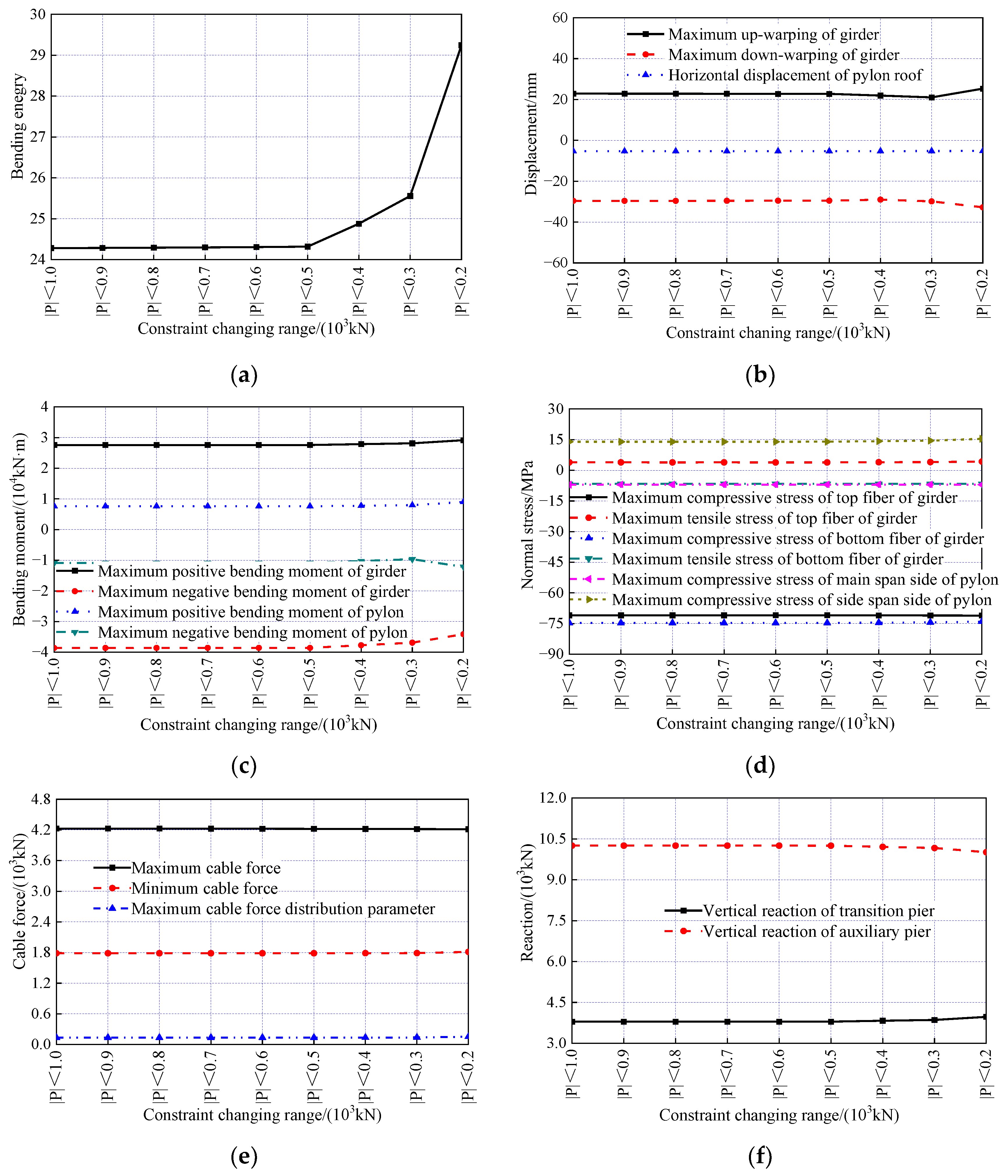
7.4. The Influence of the Constraint Range for Cable Force Uniformity on the Optimization Results

Holding all of the other constraints constant, the effect of varying the cable force uniformity constraint from $1600 \mathrm{kN}\le T_{\mathrm{i}}\le 0.4T_{\mathrm{pdi}}$ to $2000 \mathrm{kN}\le T_{\mathrm{i}}\le 0.4T_{\mathrm{pdi}}$ on the optimization outcomes is investigated. The variations in the structural states resulting from decreasing the cable force uniformity constraint range are presented in Figure 20. Variations in the cable force uniformity constraint significantly affect the main beam’s maximum deflections, the maximum bending moments, the maximum tensile stresses at the top and bottom edges, the maximum bending moments in the pylons, and the maximum cable force distribution parameter. The impact on the other structural characteristics is less than 5%. In particular, the maximum positive bending moment in the main beam, the maximum tensile stress at the bottom edge of the main beam, and the maximum cable force distribution parameter all increase with a decreasing range of constraints on the cable force uniformity. The maximum negative bending moment in the main beam decreases with a decreasing range. The main beam’s vertical displacement, the maximum tensile stress at the top edge of the main beam, and the maximum positive and negative bending moments in the pylons initially decrease and then increase with a decreasing range. Crucially, the results indicate that a cable force uniformity constraint of $\left|P_{\mathrm{i}}\right|\le 300 \mathrm{kN}$ yields a smoother structural profile, smaller maximum positive and negative bending moments in the main beam and pylons, and a lower maximum cable force distribution parameter, suggesting the suitability of this constraint range.

Based on the foregoing analysis, for the Xiangshan Port cable-stayed bridge with steel box girders, the vertical displacement of the main girder, the positive and negative bending moments, and the normal stresses at the top and bottom edges, as well as the positive and negative bending moments in the towers, are significantly influenced by the constraint ranges. The horizontal displacement of the pylon roof is significantly affected by the constraint ranges of both the main girder’s vertical displacement and the pylon’s horizontal displacement, while the effects of the other two constraint ranges are comparatively minor. The four constraint ranges exhibit a limited effect on the stresses on both sides of the pylon.

8. Conclusions

Using the Xiangshan Port cable-stayed bridge with steel box girders as a case study, this article investigates the optimization methods for the finished state. Through introducing constraint conditions, determination of a reasonable finished state is formulated as a mixed-constraint quadratic programming problem, which is then solved using the multiplier path following algorithm. Furthermore, the influence of the constraint ranges on the optimization results is analyzed, considering the vertical displacement of the main girder, the horizontal displacement of the piers, the cable forces, and cable force uniformity. The principal conclusions are summarized below:

(1) Convergence of the objective function is achieved within 30 iterations of the mixed-constraint quadratic programming model. The optimized profile of the main girder is smooth, with a uniform stress distribution along the top and bottom flanges; the top of the pylon exhibits a predetermined lateral offset towards the outer span, with a fully compressed cross-section; the cable forces increase uniformly with cable length; and positive vertical support reactions are observed in both transition and auxiliary piers, indicating sufficient pressure reserves. This suggests the reasonableness of the constraint range and the feasibility and efficiency of the optimization method for the finished state.

(2) The multiplier path following optimization algorithm is computationally efficient, exhibiting good convergence and insensitivity to the problem size. Being easy to program, it avoids the arbitrariness of manual cable adjustments, enabling straightforward determination of the reasonable finished state for a cable-stayed bridge with steel box girders. The optimized results provide a theoretical benchmark for the design of cable-stayed bridges with steel box girders.

(3) Regarding the Xiangshan Port cable-stayed bridge with steel box girders, the vertical displacement of the main girder, the positive and negative bending moments, and the normal stresses at the top and bottom edges, as well as the positive and negative bending moments in the towers, are significantly influenced by the constraint ranges. The horizontal displacement of the pylon roof is significantly affected by the constraint ranges of both the main girder’s vertical displacement and the pylon’s horizontal displacement, while the remaining constraint ranges have a limited impact.

References

1. Šurdilović, S.M.; Živković, S.; Turnić, D. Algorithms for Computer-Based Calculation of Individual Strand Tensioning in the Stay Cables of Cable-Stayed Bridges. Appl. Sci. 2024, 14, 5410. [Google Scholar] [CrossRef]
2. Yao, Y.C.; Pu, H.Q.; Yao, D.Y. Mechanical Features of Cable-Girder Anchorage for Long-Span Railway Cable-Stayed Bridge with Steel Box Girders. Appl. Mech. Mater. 2014, 3308, 1391–1394. [Google Scholar] [CrossRef]
3. Shi, J.; Chen, Z. Research on Reasonable Construction Plan for Cast-in-Place UHPC Bridge Deck Plate of Cable-Stayed Bridge. Appl. Sci. 2023, 13, 8615. [Google Scholar] [CrossRef]
4. Martins, M.A.; Simões, M.L.; Negrão, H.J. Optimization of cable-stayed bridges: A literature survey. Adv. Eng. Softw. 2020, 149, 102829. [Google Scholar] [CrossRef]
5. Ma, Y.; Song, C.; Wang, Z.P.; Jiang, Z.Q.; Sun, B.; Xiao, R.C. Efficient Design Optimization of Cable-Stayed Bridges: A Two-Layer Framework with Surrogate-Model-Assisted Prediction of Optimum Cable Forces. Appl. Sci. 2024, 14, 2007. [Google Scholar] [CrossRef]
6. Podolny, W.; Fleming, J.F. Historical Development of Cable-Stayed Bridges. J. Struct. Div. 1972, 98, 2079–2095. [Google Scholar] [CrossRef]
7. Chatterjee, S. The Design of Modern Steel Bridges, 2nd ed.; Blackwell Science Ltd.: Berlin, Germany, 2003. [Google Scholar]
8. Lin, Y.P. Cable-Stayed Bridge; China Communications Press: Beijing, China, 2004. (In Chinese) [Google Scholar]
9. Wang, P.H.; Tseng, T.C.; Yang, C.G. Initial shape of cable-stayed bridges. Comput. Struct. 1993, 47, 111–123. [Google Scholar] [CrossRef]
10. Chen, D.W.; Au, F.T.K.; Tham, L.G.; Lee, P.K.K. Determination of initial cable forces in prestressed concrete cable-stayed bridges for given design deck profiles using the force equilibrium method. Comput. Struct. 2000, 74, 1–9. [Google Scholar] [CrossRef]
11. Yan, D.H.; Li, X.W.; Liu, G.D.; Yi, W.J. Deciding the reasonable finished dead state of the main beam of cable-stayed bridges using stress balanced method. China J. Highw. Transp. 2000, 13, 49–52. (In Chinese) [Google Scholar]
12. Janjinc, D.; Pircher, M.; Pircher, H. Optimization of cable tensioning in cable-stayed bridges. J. Bridge Eng. 2003, 8, 131–137. [Google Scholar] [CrossRef]
13. Liang, P.; Xiao, R.C.; Zhang, X.S. Practical method of optimization of cable tensions for cable-stayed bridge. J. Tongji Univ. 2003, 31, 1270–1274. (In Chinese) [Google Scholar]
14. Kasuga, A.; Arai, H.; Breen, J.E.; Furukawa, K. Optimum cable-force adjustments in concrete cable-stayed bridges. J. Struct. Eng. 1995, 121, 685–694. [Google Scholar] [CrossRef]
15. Xiao, R.C.; Xiang, H.F. Influence matrix method of cable tension optimization for cable-stayed bridges. J. Tongji Univ. 1998, 26, 235–240. (In Chinese) [Google Scholar]
16. Lute, V.; Upadhyay, A.; Singh, K.K. Genetic algorithms-based optimization of cable stayed bridges. J. Softw. Eng. Appl. 2011, 4, 571–578. [Google Scholar] [CrossRef]
17. Hassan, M.M. Optimum Design of Cable-Stayed Bridges. Ph.D. Thesis, University of Western Ontario, London, ON, Canada, 2010. [Google Scholar]
18. Hassan, M.M. Optimization of stay cables in cable-stayed bridges using finite element, genetic algorithm, and B-spline combined technique. Eng. Struct. 2013, 49, 643–654. [Google Scholar] [CrossRef]
19. Sung, Y.C.; Chang, D.W.; Teo, E.H. Optimization post-tensioning cable forces of Mau-Lo Hsi cable-stayed bridge. Eng. Struct. 2006, 28, 1407–1417. [Google Scholar] [CrossRef]
20. Wilson, R.B. A Simplicial Method for Concave Programming. Ph.D. Thesis, Harvard University, Cambridge, MA, USA, 1963. [Google Scholar]
21. Han, S.P. Superlinearly Convergent Variable Metric Algorithms for General Nonlinear Programming Problems. Math. Program. 1976, 11, 263–282. [Google Scholar] [CrossRef]
22. Powell, M.J.D. A fast algorithm for nonlinearly constrained optimization calculations. In Numerical Analysis; Lecture Notes in Mathematics; Springer: Berlin/Heidelberg, Germany, 1978; p. 630. [Google Scholar]
23. Powell, M.J.D. Algorithms for nonlinear constraints that use lagrangian functions. Math. Program. 1978, 14, 224–248. [Google Scholar] [CrossRef]
24. Xiao, R.C.; Hai, F.X. Optimization Method of Cable Prestresses of Cable-Stayed Bridges and Its Engineering Applications. Chin. J. Comput. Mech. 1998, 15, 118–126. [Google Scholar]
25. Lonetti, P.; Pascuzzo, A. Design Analysis of the Optimum Configuration of Self-Anchored Cable Stayed Suspension Bridges. Struct. Eng. Mech. 2014, 51, 847–866. [Google Scholar] [CrossRef]
26. Lonetti, P.; Pascuzzo, A. Optimum Design Analysis of Hybrid Cable-Stayed Suspension Bridges. Adv. Eng. Softw. 2014, 73, 53–66. [Google Scholar] [CrossRef]
27. Hassan, M.; Nassef, A.O.; El Damatty, A.A. Determination of Optimum Post-Tensioning Cable Forces of Cable Stayed Bridges. Eng. Struct. 2012, 44, 248–259. [Google Scholar] [CrossRef]
28. Manh, H.H.; Quoc, A.V.; Viet, H.T. Optimum Design of Stay Cables of Steel Cable-stayed Bridges Using Nonlinear Inelastic Analysis and Genetic Algorithm. Structures 2018, 16, 288–302. [Google Scholar]
29. Guo, J.J.; Yuan, W.C.; Dang, X.Z.; Alam, M.S. Cable force optimization of a curved cable-stayed bridge with combined simulated annealing method and cubic B-Spline interpolation curves. Eng. Struct. 2019, 201, 109813. [Google Scholar] [CrossRef]
30. Sung, Y.C.; Wang, C.Y.; Teo, E.H. Application of particle swarm optimisation to construction planning for cable-stayed bridges by the cantilever erection method. Struct. Infrastruct. Eng. 2016, 12, 208–222. [Google Scholar] [CrossRef]
31. Wang, L.F.; Xiao, Z.W.; Li, M.; Fu, N. Cable Force Optimization of Cable-Stayed Bridge Based on Multiobjective Particle Swarm Optimization Algorithm with Mutation Operation and the Influence Matrix. Appl. Sci. 2023, 13, 2611. [Google Scholar] [CrossRef]
32. Lei, L.H. Exploration of optimization design for cable force of cable-stayed bridge. J. China Foreign Highw. 2006, 26, 77–80. (In Chinese) [Google Scholar]
33. Powell, M.J.D. A Method for Nonlinear Constraints in Minimization Problems. In Optimization; Fletcher, R., Ed.; Academic Press: New York, NY, USA, 1969; pp. 283–298. [Google Scholar]
34. Hestenes, M.R. Multiplier and gradient methods. J. Optim. Theory Appl. 1969, 4, 303–320. [Google Scholar] [CrossRef]
35. Karmarkar, N. A new polynomial-time algorithm for linear programming. Combinatorica 1984, 4, 373–395. [Google Scholar] [CrossRef]
36. Lu, Z.S.; Monteiro, R.D.C. An iterative solver-based long-step infeasible primal-dual path-following algorithm for convex QP based on a class of preconditioners. Optim. Methods Softw. 2009, 24, 123–143. [Google Scholar] [CrossRef]
37. Goldfarb, D.; Liu, S. An O (n3L) primal Interior point algorithm for convex quadratic programming. Math. Program. 1991, 49, 325–340. [Google Scholar] [CrossRef]
38. Monteiro, R.D.C.; Adler, I. Interior path following primal-dual algorithm. Part I: Linear programming. Math. Program. 1989, 44, 27–41. [Google Scholar] [CrossRef]
39. Monteiro, R.D.C.; Adler, I. Interior path following primal-dual algorithm. Part II: Convex quadratic programming. Math. Program. 1989, 44, 43–66. [Google Scholar] [CrossRef]
40. Chen, B.L. Optimization Theory and Algorithm, 2nd ed.; Tsinghua University Press: Beijing, China, 2005. (In Chinese) [Google Scholar]
41. Gong, C.; Wang, Z.L. Proficient in MATLAB Optimization Calculation, 2nd ed.; Publishing House of Electronics Industry: Beijing, China, 2012. (In Chinese) [Google Scholar]
Figure 1. The iterative process based on the multiplier path following method.
Applsci 15 00937 g001
Figure 2. Optimization process of finished state for cable-stayed bridge with steel box girder.
Applsci 15 00937 g002
Figure 3. Layout of Xiangshan Port bridge (cm).
Applsci 15 00937 g003
Figure 4. Influence matrix of cable force on values of selected structural responses. (a) Vertical displacement of main girder; (b) horizontal displacement of pylon; (c) bending moment of main girder; (d) bending moment of pylon; (e) cable force.
Applsci 15 00937 g004aApplsci 15 00937 g004b
Figure 5. Displacement evoked by the unit cable force: (a) vertical (main girder); (b) horizontal (pylon).
Applsci 15 00937 g005
Figure 6. Bending moment evoked by the unit cable force in (a) the main girder and (b) the pylon.
Applsci 15 00937 g006
Figure 7. Displacement evoked by the dead load (excluding cable force): (a) vertical (main girder); (b) horizontal (pylon).
Applsci 15 00937 g007
Figure 8. Bending moment evoked by the dead load (excluding the cable force) in the (a) main girder and (b) pylon.
Applsci 15 00937 g008
Figure 9. Cable forces under dead load (excluding cable force).
Applsci 15 00937 g009
Figure 10. Evolution of the value of the objective function with the number of iterations.
Applsci 15 00937 g010
Figure 11. Optimal sequence of cable forces.
Applsci 15 00937 g011
Figure 12. Displacement evoked by the dead load. (a) Vertical (main girder); (b) horizontal (pylon).
Applsci 15 00937 g012
Figure 13. Axial force evoked by the dead load in the (a) main girder and (b) pylon.
Applsci 15 00937 g013
Figure 14. Bending moment evoked by the dead load in the (a) main girder and (b) pylon.
Applsci 15 00937 g014
Figure 15. Normal stress of selected structures under dead load. (a) Top flange of main girder; (b) side span of pylon; (c) bottom flange of main girder; (d) main span of pylon.
Applsci 15 00937 g015
Figure 16. Cable force under dead load.
Applsci 15 00937 g016
Figure 17. Variation in values of selected structural responses with decreasing constraint range of main girder’s vertical displacement. (a) Structural bending energy; (b) structural displacement; (c) structural bending moment; (d) structural normal stress; (e) cable force; (f) vertical support reaction.
Applsci 15 00937 g017aApplsci 15 00937 g017b
Figure 18. Variation in values of selected structural responses with decreasing constraint range for horizontal pylon displacement. (a) Structural bending energy; (b) structural displacement; (c) structural bending moment; (d) structural normal stress; (e) cable force; (f) vertical support reaction.
Applsci 15 00937 g018
Figure 19. Variation in values of selected structural responses with decreasing constraint range for cable force. (a) Structural bending energy; (b) structural displacement; (c) structural bending moment; (d) structural normal stress; (e) cable force; (f) vertical support reaction.
Applsci 15 00937 g019
Figure 20. Variation in values of selected structural responses with decreasing constraint range of cable force uniformity. (a) Structural bending energy; (b) structural displacement; (c) structural bending moment; (d) structural normal stress; (e) cable force; (f) vertical support reaction.
Applsci 15 00937 g020
Disclaimer/Publisher’s Note: The statements, opinions and data contained in all publications are solely those of the individual author(s) and contributor(s) and not of MDPI and/or the editor(s). MDPI and/or the editor(s) disclaim responsibility for any injury to people or property resulting from any ideas, methods, instructions or products referred to in the content.