Abstract
Air pollution concerns have led to the widespread deployment of air quality monitoring stations. While high-cost government stations provide accurate data, their deployment is limited, whereas low-cost sensors offer widespread coverage but with lower accuracy. To enhance the accuracy of measurement data from low-cost air monitoring sensors, this study proposes a Multi-Scale Convolutional Residual Time-Frequency Calibration Method (MCRTF-CM), focusing on the PM2.5 sensor as an example. This method leverages multi-scale convolution in the feature extractor to capture diverse features at various scales using parallel convolutional kernels. Residual connections merge the original and multi-scale features, preserving the initial input for enhanced stability. The calibration module employs Gated Recurrent Units (GRUs) to capture long-term dependencies in time-series data through reset and update gates. Additionally, the Frequency Enhanced Channel Attention Mechanism (FECAM) uses Discrete Cosine Transform (DCT) to convert time-domain data to frequency-domain, assigning weights to different frequency components to enhance key features and suppress irrelevant ones. Experimental results demonstrate that MCRTF-CM outperforms optimal Long Short-Term Memory (LSTM) networks, reducing RMSE, MAE, MSE, and MAPE by 13.59%, 14.04%, 25.33%, and 8.22%, respectively, indicating its better performance.
1. Introduction
With the advancement of industrialization and urbanization, air pollution has become a global environmental issue, directly impacting human health and quality of life. Prolonged exposure to air pollutants has been linked to a wide range of diseases, including cardiovascular [1], respiratory [2], and neurological disorders [3], among others, making comprehensive air quality monitoring and timely reporting essential [4].
Many cities have established national monitoring stations to release reliable Air Quality Index (AQI) data, keeping the public informed about air quality and managing pollutants. While these stations provide accurate pollutant measurements, their high installation and maintenance costs limit widespread use. To address this, regions are adopting low-cost monitoring devices with lower installation and maintenance expenses. However, these devices are more susceptible to environmental factors, such as fluctuations in temperature and humidity, which can lead to sensor drift or variations in sensitivity. Additionally, interference from other pollutants, such as ozone or carbon monoxide, can affect sensor readings, causing cross-sensitivity or inaccurate measurements. Unlike national control stations, which use calibrated, high-precision instruments and operate in controlled environments, low-cost devices may experience greater variability in their readings due to these environmental influences, ultimately resulting in less accurate data for air quality assessment compared to national control stations.
To address the issue of low accuracy in measurement data from low-cost air monitoring sensors, calibration methods are generally divided into hardware and software approaches. Hardware compensation involves building circuits to adjust for factors such as temperature and humidity that can influence sensor data [5]. However, this approach lacks flexibility and often leads to significant errors under varying environmental conditions, making it impractical for real-world calibration applications. To improve precision, software compensation methods rely on reference data collected from public air monitoring stations, often using on-site techniques to adjust sensor outputs [6]. Traditional software compensation methods, including interpolation [7], multiple linear regression [8], etc., are widely employed in this context. Kasimir Aula et al. [9] utilized interpolation to estimate missing values and smooth sensor outputs, while Karagulian et al. [10] applied multiple linear regression to account for temperature and humidity effects, improving calibration accuracy. However, traditional methods assume a linear relationship [11] between errors and environmental factors, which often fails to capture complex error patterns and adapt to sensor drift or environmental changes, leading to unstable performance in dynamic conditions. These limitations [12] have driven the adoption of machine learning-based approaches for more accurate sensor calibration.
Recently, machine learning techniques have emerged as promising alternatives to overcome these challenges. Random Forest Regression (RFR) effectively addresses cross-sensitivity [13], while Loh and Choi [14] employed methods like SVM, k-nearest neighbors, and random forests for calibration using government-approved data. Martina Casari [15] demonstrated the efficiency of multi-layer perceptrons for PM2.5 time calibration. Recurrent Neural Networks (RNNs) model historical time series but face challenges like pre-determining time delays and capturing long-term dependencies. Long Short-Term Memory (LSTM) networks [16] address these issues, as shown by studies like Chiara Bachechi [17] using HypeAIR for real-time calibration and Yu et al.’s [18] demonstration of CNN and RNN effectiveness for calibrating CO and sensors, surpassing traditional regression techniques. Linear regression is often regarded as a straightforward and intuitive approach for improving sensor accuracy. However, as noted by Moreno-Rangel et al. [19], the relationship between sensor data and reference values is not always linear or confined to a single dimension. In cases involving nonlinear and multidimensional dependencies, machine learning (ML) algorithms present a promising alternative for sensor calibration [20].
This paper focuses on calibrating low-cost air quality sensors, particularly for PM2.5 measurements. Factors such as cross-interference from varying gas concentrations and weather conditions [21], as well as zero and span drift in optical particle counters over time [22], can significantly affect the accuracy of sensor measurement data. Specifically, the presence of certain gases can lead to erroneous readings by altering the sensor’s baseline or response to particulate matter, resulting in inaccurate PM2.5 measurements. This phenomenon, known as cross-sensitivity, is a critical challenge for the reliable operation of low-cost sensors in dynamic environments. Traditional software compensation methods struggle to capture complex relationships, leading to poor fitting accuracy [23]. Therefore, developing an appropriate calibration model is crucial. Calibration of air pollution monitoring data primarily occurs at the data level, where calibration models are employed to correct the measurements.
The proposed MCRTF-CM model calibrates low-cost air quality sensor data using a feature extractor and a calibration module. The feature extractor employs multi-scale convolution with residual connections to capture and preserve temporal features, which are fused and processed by the calibration module. Utilizing a GRU, the calibration module captures temporal dependencies and dynamic changes, while the FECAM (Frequency-domain Enhanced Channel Attention Mechanism) improves feature representation. A fully connected layer generates the final output, enabling the model to achieve accurate calibration by effectively leveraging sensor data features.
To address these challenges, this paper proposes the MCRTF-CM model. The main contributions are as follows:
- The feature extractor in the MCRTF-CM model utilizes a multi-scale convolutional structure to capture features across different temporal scales from sensor data. Through residual connections, the model effectively preserves critical information while reducing cross-interference from other features, enhancing feature richness and calibration accuracy.
- The GRU (Gated Recurrent Unit) in the calibration module leverages gating mechanisms to control information flow and updates, effectively capturing temporal dependencies and dynamic changes in sensor data. This enhances the model’s ability to utilize historical data, improving calibration accuracy in dynamic environments.
- Time-domain calibration is commonly used due to its directness and broad applicability, but it may struggle with noise. To enhance calibration performance, the MCRTF-CM model incorporates a FECAM (Frequency-domain Enhanced Channel Attention Mechanism). This module uses frequency-domain analysis to improve feature representation, effectively suppressing noise and irrelevant frequency components, enabling more accurate capture and utilization of key information for high-precision calibration.
2. Proposed Method
2.1. MCRTF-CM
This paper presents a calibration method for low-cost air sensors, named MCRTF-CM, which consists of two main components: a feature extractor and a calibration module. The model structure is illustrated in Figure 1.
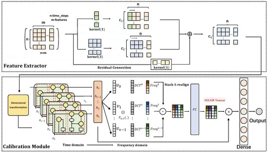
Figure 1.
Framework of MCRTF-CM.
In the feature extraction stage, 11 features—PM2.5, PM10, CO, , , , and five meteorological factors (temperature, wind speed, humidity, pressure, and rainfall)—along with the corresponding window size, are input into the model. Multi-scale convolutional layers with residual connections are employed to capture both short-term and long-term temporal information via parallel convolutions with varying kernel sizes. The residual connections ensure shallow-layer inputs are preserved, facilitating gradient [24] propagation and retaining essential original information at deeper layers, thus mitigating cross-interference effects on the sensor data.
In the calibration module, a combination of time-domain and frequency-domain approaches is utilized. The GRU captures temporal dependencies, while the DCT transforms time-domain data into the frequency domain, where the FECAM assigns weights across different frequency scales to emphasize critical information and suppress noise. The final sensor readings are calibrated through a fully connected layer.
2.2. Feature Extractor
Convolutional Neural Networks (CNNs) [25] are a type of feedforward neural network primarily comprising convolutional layers. These layers perform convolution operations to extract deep features and enable parameter sharing, which reduces network complexity and training costs. CNNs effectively extract hierarchical features from PM2.5 and other variables, thereby improving calibration accuracy. The structure of the CNN is illustrated in Figure 2.
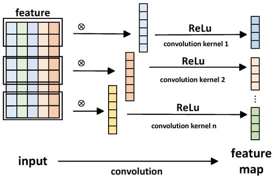
Figure 2.
The diagram of CNN feature extraction.
Convolutional layers are central to CNNs, performing convolution operations on input data through local connections and weight sharing to extract deep features. Given input data , the convolution process is defined by
where represents the feature map obtained by convolving the input data with the k-th kernel, where and are the kernel’s weights and bias, respectively. Here, g is the kernel size, n is the sensor sequence length, and m is the number of sequences. The ReLU activation function is then applied to introduce nonlinearity, producing the final features extracted by the convolutional layer.
Residual Neural Networks (ResNet) are deep learning models that enhance network learning capacity [26]. The basic unit of the ResNet is the residual block, which introduces an identity mapping directly from input to output, as shown in Figure 3. This connection allows original input information [27] to flow through subsequent layers, enhancing feature representation and mitigating the vanishing gradient problem. To ensure consistent data dimensions in the residual connection, a CNN module is used for adjustment. The mathematical expression for the residual block is as follows:
where x is the original input from the skip connection, F(x) is the network’s output, and y is the residual block output, defined as F(x) + x.
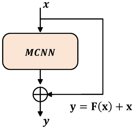
Figure 3.
ResNet structure.
2.3. Calibration Module
After feature extraction, the key step is data calibration. The calibration module combines the GRU and FECAM, followed by a fully connected layer to output the calibrated values.
LSTM [28] is used for analyzing time series data, addressing the gradient explosion and vanishing problems in RNNs [29]. The GRU [30], an improvement on LSTM, incorporates only a reset gate and an update gate. While both offer similar prediction accuracy, the GRU converges faster and is more computationally efficient. The reset gate integrates current input with past information, while the update gate preserves memory across time steps. The GRU neural network structure is shown in Figure 4, with the mathematical formulation provided in Equations (4)–(7).
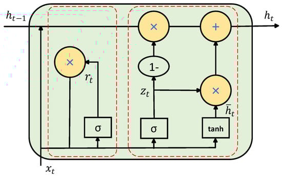
Figure 4.
The network structure of the GRU model.
In the equations: is the update gate; is the reset gate; is the hidden layer output; is the combination of input and previous hidden state ; , , , , , are trainable matrices; , , are the biases; is the sigmoid function; and tanh is the activation function.
The GRU excels in modeling time-domain data, capturing long-term dependencies in time series, but it overlooks frequency-domain information, which can reveal features that are hard to detect in the time domain. Frequency analysis can uncover valuable insights, especially when noise obscures signals, making it difficult to distinguish patterns in the time domain. By modeling in both time and frequency domains, periodic features can be captured, providing a more comprehensive feature representation and improving overall model performance.
To address the limitations of time-domain modeling, frequency information is introduced via Discrete Cosine Transform (DCT) [31]. The Frequency-domain Enhanced Channel Attention Mechanism (FECAM) [32] leverages frequency-domain modeling to assign channel weights, learning the significance of different frequencies for each channel. Frequency analysis is a natural complement to time series analysis, yet most models overlook its impact, failing to capture inherent features. Traditional methods based on Fourier Transform (FT) [33] and Inverse Fourier Transform (IFT) [34] often introduce high-frequency noise due to the Gibbs phenomenon. In contrast, the FECAM avoids these issues by capturing more time-series information through DCT, which extracts additional frequency components and automatically learns the importance of each channel while suppressing irrelevant features. This enhances the learning of inter-channel dependencies through frequency-domain modeling. The structure of the FECAM is shown in Figure 5.
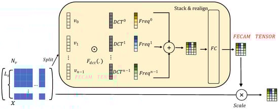
Figure 5.
Structure diagram of FECAM.
The FECAM divides the input feature map into n subsets along the channel dimension, denoted as , where = , and . Each subset is then processed with Discrete Cosine Transform (DCT) frequency components from low to high, with each channel undergoing the same frequency processing.
For and , where j is the 1D index of the frequency component in , and is the L-dimensional vector after Discrete Cosine Transform (DCT). The entire channel vector is obtained through stacking these components.
where represents the attention vector for . The complete framework of the Frequency–domain Enhanced Channel Attention Mechanism can be expressed as
This approach enables interaction between each channel feature and frequency component, comprehensively capturing important temporal information in the frequency domain, which enhances feature diversity. The fully connected layer further processes the frequency-domain features through linear transformation and nonlinear activation, emphasizing significant components, suppressing irrelevant features, and reducing noise.
2.4. Detailed Settings of MCRTF-CM
The model was trained using Mean Squared Error (MSE) as the loss function. To eliminate scale differences between features, input data were preprocessed using Scikit-Learn’s MinMaxScaler [35] before being fed into the MCRTF-CM model. The Adam optimizer [36] with a learning rate of 0.01 was employed during training. To prevent overfitting, dropout [37] with a probability of 0.1 was applied, and the input sequence window length was set to 24. Other parameters are detailed in Table 1.

Table 1.
Parameters of the MCRTF-CM model.
3. Experimental Results and Analysis
The proposed neural network was implemented in PyTorch using Python 3.7.0 and executed on a high-performance computing platform with Intel(R) Iris(R) Xe Graphics CPU for computation and analysis.
3.1. Data Source and Preprocessing
This study uses air quality data from 14 November 2018 to 11 June 2019 as the dataset [38]. This paper proposes a method for calibrating low-cost sensors for PM2.5 measurements. A low-cost sensor developed by a certain company is used as an example in this study. To calibrate the PM2.5 sensor, a low-cost station equipped with air quality and meteorological sensors was developed. This station enables real-time grid-based air quality monitoring in a specific region and simultaneously measures meteorological parameters such as temperature, humidity, wind speed, pressure, and precipitation. The dataset used for calibration consists of hourly measurements collected by the self-developed low-cost station during the period from 14 November 2018 to 11 June 2019 (Table 2). The low-cost station was located near a national control point (reference station), and the PM2.5 data measured by the reference station during the same period were used to validate the PM2.5 measurements obtained from the low-cost sensor calibrated with the proposed method. Data were collected at 1-h intervals based on national control points, resulting in 5022 data entries. The dataset consists of 11 features, including PM2.5, PM10, CO, , , , and meteorological parameters such as temperature, wind speed, humidity, pressure, and precipitation. Since various pollutants and meteorological factors can affect PM2.5 measurements, these features were input into the calibration model to enhance PM2.5 accuracy.
Table 2.
Feature samples.
To improve the model’s convergence speed and calibration accuracy, the raw data were preprocessed. This involved removing missing values, normalization and denormalization, and splitting the data into training and test sets. During data collection, environmental factors like temperature, wind speed, humidity, pressure, and precipitation affected the monitoring equipment, leading to missing or anomalous data. For example, while the reference station (national control point) was supposed to record data hourly for 5021 h, only 4200 h of data were available, leaving 821 h missing. Assuming no sudden weather changes, missing values were imputed using the average of neighboring data points. The low-cost air quality sensors (self-built stations) recorded data every 5 min. To match the reference station’s hourly data, the self-built station data were resampled to hourly intervals by averaging. The resulting hourly data were then compared to the reference station data to analyze their differences.
Due to the varying scales of features in the air quality data, differences in magnitude can reduce the model’s accuracy and convergence speed. Therefore, the sample data were normalized using the Min-Max method, mapping values between 0 and 1, as shown in the following formula:
where represents the normalized data, x is the original sample data, and and are the maximum and minimum values of the sample data, respectively.
To ensure the predicted results are meaningful, the calibration results were denormalized using the following formula:
After these processes, the input time series for model training was constructed by selecting data from 15 November 2018 to 1 May 2019 as the training set and from 1 May 2019 to 11 June 2019 as the test set, with an 8:2 training-to-testing ratio.
3.2. Correlation Between Different Pollutants and Meteorological Factors
Due to the influence of sensors at monitoring stations and the mutual impact between different pollutants and meteorological factors, there is a certain degree of correlation among various pollutants. As shown in Figure 6, the Pearson correlation coefficient [39] is used to measure the correlation between different variables, and it is presented intuitively in the form of a heatmap [40]. The horizontal and vertical axes in the figure list six pollutants and five meteorological factors monitored by the microstation, with the colored rectangles indicating the correlation between the pollutants on each axis. The closer the value in the rectangle is to 1, the stronger the positive correlation; conversely, values closer to −1 indicate a stronger negative correlation.
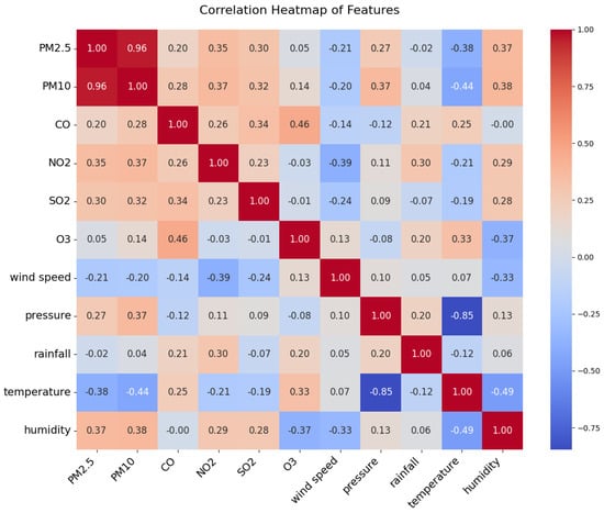
Figure 6.
The correlation between pollutant monitoring data and meteorological factors.
The analysis indicates that when monitoring pollutant data with microstation sensors, PM2.5 shows a positive correlation of 0.96 with PM10 and a negative correlation of 0.38 with temperature. CO has a positive correlation of 0.46 with and a negative correlation of 0.4 with . The figure confirms that there is significant cross-interference among pollutants monitored by the microstation sensors, with data mutually impacting each other and substantially affecting monitoring accuracy. Additionally, meteorological factors also influence various pollutants. Therefore, when calibrating the data, it is essential to fully consider the interactions between different pollutants and the effects of weather to minimize their impact on data correction.
3.3. Evaluation Metrics
To assess the calibration performance of the model, four traditional evaluation metrics were used: Mean Absolute Error (MAE), Root Mean Squared Error (RMSE), Mean Squared Error (MSE), and Mean Absolute Percentage Error (MAPE). Smaller values of MAE, RMSE, MSE, and MAPE indicate higher accuracy of the calibration model. The corresponding formulas are as follows:
- (1)
- Mean Absolute Error (MAE):
- (2)
- Root Mean Squared Error (RMSE):
- (3)
- Mean Squared Error (MSE):
- (4)
- Mean Absolute Percentage Error (MAPE)
In the formula, n represents the total number of calibration values, denotes the actual PM2.5 values, and denotes the calibrated PM2.5 values.
3.4. Experimental Results
To evaluate the effectiveness of the MCRTF-CM model in calibrating low-cost air quality sensors, we compared its calibration errors with six other models: random forest (RF), support vector regression (SVR), multi-layer perceptron (MLP), multiple linear regression (MLR), extreme gradient boosting (XGBoost), and Long Short-Term Memory (LSTM). These models were implemented using open-source libraries, with necessary adjustments to suit the specific characteristics of the dataset. The implementation was optimized and adjusted according to the specific requirements of the experiments, and the hyperparameters for each model were fine-tuned to ensure optimal performance. To ensure fairness, all models were tested on the same dataset with identical preprocessing methods. Each model was trained 20 times with optimal hyperparameters to mitigate result variability, and the average calibration value was used. Uncalibration results, calibration results, and reference results are visualized in Figure 7, where points closer to the diagonal reference line indicate smaller errors and better calibration performance. Due to the large and complex test set data, we selected a subset from 24 May 2019 12:00 to 24 May 2019 20:00 to illustrate the calibration values and actual values for the seven models, as shown in Figure 8. Figure 9 illustrates the variation of calibrated values from different models compared to the reference values using error bars. The error bars represent the standard deviation of the residuals, where residuals are the differences between the calibrated values and the true values. The standard deviation reflects the distribution of the residuals, indicating the degree of dispersion of the calibrated values relative to the true values. Additionally, the coverage ratio for each model was calculated, representing the proportion of reference values falling within the error range of the calibrated values. Specifically, the coverage ratio is determined by checking whether the reference values lie within the range of the calibrated value ± error bar (i.e., standard deviation). To further verify the reasonableness of the calibration values of these seven models, both error bars and coverage ratios are utilized. If the error bars include the reference value, the calibration values are considered within a reasonable range. The coverage ratio indicates the proportion of error bars that include the reference value. As shown in Figure 9, the error bars are reasonable. This approach provides a more comprehensive assessment of the calibration performance of each model by considering not only the absolute calibration error but also the consistency of calibration results over different periods. The incorporation of error bars and coverage ratios offers a deeper evaluation of model performance and an understanding of calibration uncertainty.
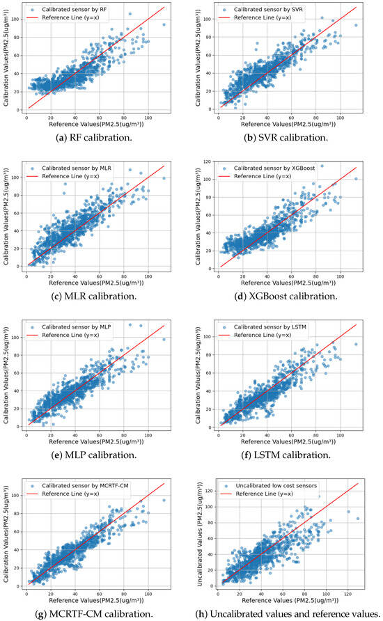
Figure 7.
Scatter plots of the calibrated values and reference values for the seven models, as well as scatter plots of the uncalibrated values and reference values.
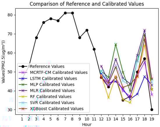
Figure 8.
Calibration plots for seven models.
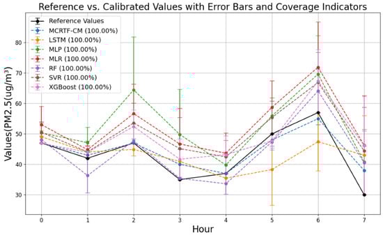
Figure 9.
Reference vs. calibrated values with error bars and coverage indicators.
Table 3 presents the test results for each model on the data from 22 May 2019 12:00:00 to 11 June 2019 15:00:00. The MCRTF-CM model achieved superior calibration performance, with reductions in the MAE, RMSE, MSE, and MAPE compared to the best-performing models. Specifically, MCRTF-CM reduced the MAE, RMSE, MSE, and MAPE by 14.04%, 13.59%, 25.33%, and 8.22%, respectively, compared to LSTM, and by 18.24%, 14.89%, 27.57%, and 24.10%, respectively, compared to MLP. This indicates that the MCRTF-CM model has better feature extraction and nonlinear mapping capabilities.
Table 3.
Comparison of evaluation metrics across models.
3.5. Ablation Study
To assess the importance of different features and modules in our method, ablation studies were conducted on both the feature and module components.
(1) Feature-level Ablation Study: The input features include internal and external factors, with the latter divided into other air pollutants and weather-related factors. To evaluate the impact of these external factors on model performance, we conducted an ablation study by removing each type of external factor from the initial feature set. The performance of the MCRTF-CM model was then assessed with the remaining features. The model with other air pollutant features removed is denoted as MCRTF-CM(AF), and the model with weather-related features removed is denoted as MCRTF-CM(WF).
Table 4 summarizes the experimental results. Removing other air pollutants (except PM2.5) resulted in MCRTF-CM(AF) showing increases in the MAE, RMSE, MSE, and MAPE by 12.44%, 11.14%, 23.52%, and 16.75%, respectively, compared to MCRTF-CM. This indicates that the features of other pollutants enhance model performance. The correlation between different pollutants suggests that PM2.5 sensor readings may be indirectly influenced by these pollutants. Specifically, pollutants such as PM10, CO, , , and are often found to be temporally and spatially correlated with PM2.5 concentrations, as they share similar sources and atmospheric behaviors. For instance, high concentrations of and may indicate urban emissions, which also contribute to the formation of fine particulate matter. Removing these pollutant features reduces the amount of information available to the model, resulting in decreased calibration accuracy for PM2.5.
Table 4.
Ablation study of different factors.
On the other hand, removing weather-related features led to reductions in the MAE, RMSE, MSE, and MAPE by 27.06%, 25.66%, 44.74%, and 27.29% compared to MCRTF-CM(AF). This result demonstrates that weather conditions, particularly temperature, humidity, and wind speed, have a more significant impact on the calibration of PM2.5 sensors. Weather variables influence the dispersion, dilution, and deposition of airborne particles, thereby affecting the observed concentration of PM2.5. For instance, high humidity levels can increase particle size, making them easier to detect, while temperature and wind speed can influence the vertical mixing and horizontal transport of particulate matter. Therefore, it is crucial to consider both pollutant and weather-related features in air quality monitoring systems to enhance model accuracy and reliability.
(2) Module-level Ablation Study: This section evaluates the importance of each module in the model through ablation experiments. Eight variants of the model, denoted as Models 1–8, were created based on different module removals. Model 1 omits the convolutional kernels and residual connections; Model 2 omits the convolutional kernels and residual connections; Model 3 omits the convolutional kernels; Model 4 omits the convolutional kernels; Model 5 omits the residual connections; Model 6 omits the FECAM; Model 7 omits both multi-scale convolution and residual connections; and Model 8 includes only the GRU. All the models were tested using the same dataset and hyperparameters from 22 May 2019 12:00:00 to 11 June 2019 15:00:00. Each network was trained 10 times, and the average results were used for calibration, as summarized in Table 5.
Table 5.
Ablation study of different modules.
As shown in Table 5, Model 8 shows an increase of 13.75%, 14.79%, 29.41%, and 12.00% in RMSE, MAE, MSE, and MAPE, respectively, compared to the MCRTF-CM model. Model 5 also shows a significant performance drop. The use of residual connections in this model retains original input information, enriching the output representation by adding this information to the model’s outputs. Residual connections facilitate gradient flow, alleviating the vanishing gradient problem and accelerating model convergence, making the network easier to train. However, a multi-scale convolutional network alone is insufficient to fully capture temporal features in sequences. Model 6, which removes the FECAM, shows a performance decrease with the RMSE, MAE, MSE, and MAPE increasing by 6.52%, 7.05%, 13.48%, and 2.85%, respectively, compared to MCRTF-CM, indicating that introducing Discrete Cosine Transforms in the frequency domain extracts features not easily detectable in the time domain. Models 1–4, retaining most of the MCRTF-CM structure, exhibit relatively smaller performance drops, further validating the effectiveness of combining convolutional networks with feature extraction and learning in both time and frequency domains. The MCRTF-CM model excels by thoroughly exploiting various sequence features, learning long-term dependencies among features, and suppressing irrelevant features in the frequency domain, resulting in the best performance.
4. Conclusions
This paper conducts calibration research on the low performance of low-cost air quality sensors in monitoring air pollutants, using high-precision government monitoring station data as reference features to learn the time-series characteristics of air pollutant data collected by low-cost sensors. The study focuses on calibrating a specific low-cost PM2.5 sensor. A calibration method based on the MCRTF-CM network is proposed, which takes various air pollutant gases and meteorological features as inputs and utilizes a multi-scale convolutional residual network to extract diverse features from the sensor data, ensuring that more original information is retained and leveraged at deeper network layers. The extracted features are then fed into a GRU network to capture long-term dependencies in the temporal dimension. Additionally, a FECAM is employed to detect periodicity and trends in the time-series data through frequency-domain transformation, which are challenging to capture directly in the time domain. By integrating both time-domain and frequency-domain learning, the MCRTF-CM model effectively maps the measurements from low-cost sensors and additional features to national standard air quality data, thereby enhancing calibration accuracy. Test results show that the MCRTF-CM model outperforms other models in calibrating low-cost air quality data, demonstrating superior performance and robustness across various evaluation metrics.
Despite the significant findings of this study, some limitations must be considered. First, the calibration model was primarily validated in specific regions and specific pollutants, limiting its generalizability to other regions and pollutants. Future research should focus on testing the model in more diverse environmental conditions, with a broader range of sensor types and pollutants, to assess its adaptability and robustness. Additionally, the issue of sensor drift over long-term use remains a critical challenge, as the performance of low-cost sensors may degrade over time. Addressing this issue will require the development of more effective calibration techniques to account for sensor aging and environmental factors. Furthermore, while the current model performs well under the conditions tested, exploring potential improvements in model scalability and computational efficiency is an important direction for future work. These efforts will help extend the applicability of the MCRTF-CM model to real-world air quality monitoring systems on a larger scale.
Author Contributions
Conceptualization, J.L. and F.S.; methodology, J.L.; software, J.L.; validation, J.L. and Z.J.; formal analysis, J.L., Z.J. and J.Q.; investigation, J.L., Z.J. and J.Q.; resources, J.Q.; data curation, J.L.; writing—original draft preparation, J.L.; writing—review and editing, J.L., F.S., Z.J. and J.Q.; visualization, J.L.; supervision, F.S.; project administration, J.L.; funding acquisition, F.S. All authors have read and agreed to the published version of the manuscript.
Funding
This work was supported by the Key Research and Development Program of Xinjiang Uygur Autonomous Region: Research and Development of Key Technologies for Calculation, Measurement, and Digitized Management of Carbon Emission and Carbon Sink Indicators in the Energy Sector (No. 2022B01010), the National Natural Science Foundation of China (No. 62261053), Tianshan Talent Training Project—Xinjiang Science and Technology Innovation Team Program (2023TSYCTD0012), and the Tianshan Innovation Team Program of Xinjiang Uygur Autonomous Region of China (2023D14012).
Institutional Review Board Statement
Not applicable.
Informed Consent Statement
Not applicable.
Data Availability Statement
The dataset used is in the public domain.
Conflicts of Interest
The authors declare no conflicts of interest.
References
- Al-Kindi, S.G.; Brook, R.D.; Biswal, S.; Rajagopalan, S. Environmental determinants of cardiovascular disease: Lessons learned from air pollution. Nat. Rev. Cardiol. 2020, 17, 656–672. [Google Scholar] [CrossRef]
- Lee, Y.G.; Lee, P.H.; Choi, S.M.; An, M.H.; Jang, A.S. Effects of air pollutants on airway diseases. Int. J. Environ. Res. Public Health 2021, 18, 9905. [Google Scholar] [CrossRef] [PubMed]
- Sethi, Y.; Agarwal, P.; Vora, V.; Gosavi, S. The impact of air pollution on neurological and psychiatric health. Arch. Med. Res. 2024, 55, 103063. [Google Scholar] [CrossRef] [PubMed]
- Ganesh, C.S.; Prasaath, V.A.; Arun, A.; Bharath, M.; Kanagasabapathy, E. Internet of Things Enabled Air Quality Monitoring System. In Proceedings of the 2023 IEEE International Conference on Sustainable Computing and Smart Systems (ICSCSS), Coimbatore, India, 14–16 June 2023; pp. 934–937. [Google Scholar]
- Abdullah, A.N.; Kamarudin, K.; Mamduh, S.M.; Adom, A.H.; Juffry, Z.H.M. Effect of environmental temperature and humidity on different metal oxide gas sensors at various gas concentration levels. In Proceedings of the IOP Conference Series: Materials Science and Engineering. IOP Publishing, Bangkok, Thailand, 4–5 February 2020; Volume 864, p. 012152. [Google Scholar]
- Koziel, S.; Pietrenko-Dabrowska, A.; Wojcikowski, M.; Pankiewicz, B. On Memory-Based Precise Calibration of Cost-Efficient NO2 Sensor Using Artificial Intelligence and Global Response Correction. Knowl.-Based Syst. 2024, 290, 111564. [Google Scholar] [CrossRef]
- Wu, T.; Chen, S.; Wu, P.; Nie, S. A high precision software compensation algorithm for silicon piezoresistive pressure sensor. Chin. J. Electron. 2019, 28, 748–753. [Google Scholar] [CrossRef]
- Xu, W.; Feng, X.; Xing, H. Modeling and analysis of adaptive temperature compensation for humidity sensors. Electronics 2019, 8, 425. [Google Scholar] [CrossRef]
- Aula, K.; Lagerspetz, E.; Nurmi, P.; Tarkoma, S. Evaluation of low-cost air quality sensor calibration models. ACM Trans. Sens. Netw. 2022, 18, 1–32. [Google Scholar] [CrossRef]
- Karagulian, F.; Barbiere, M.; Kotsev, A.; Spinelle, L.; Gerboles, M.; Lagler, F.; Redon, N.; Crunaire, S.; Borowiak, A. Review of the performance of low-cost sensors for air quality monitoring. Atmosphere 2019, 10, 506. [Google Scholar] [CrossRef]
- Allegrini, F.; Olivieri, A.C. Linear or non-linear multivariate calibration models? that is the question. Anal. Chim. Acta 2022, 1226, 340248. [Google Scholar] [CrossRef] [PubMed]
- Ren, L.; Cheng, G.; Chen, W.; Li, P.; Wang, Z. Advances in drift compensation algorithms for electronic nose technology. Sensor Rev. 2024, 44, 733–745. [Google Scholar] [CrossRef]
- Zimmerman, N.; Presto, A.A.; Kumar, S.P.; Gu, J.; Hauryliuk, A.; Robinson, E.S.; Robinson, A.L.; Subramanian, R. A machine learning calibration model using random forests to improve sensor performance for lower-cost air quality monitoring. Atmos. Meas. Tech. 2018, 11, 291–313. [Google Scholar] [CrossRef]
- Loh, B.G.; Choi, G.H. Calibration of portable particulate matter–monitoring device using web query and machine learning. Saf. Health Work 2019, 10, 452–460. [Google Scholar] [CrossRef]
- Casari, M.; Po, L.; Zini, L. AirMLP: A Multilayer Perceptron Neural Network for Temporal Correction of PM2.5 Values in Turin. Sensors 2023, 23, 9446. [Google Scholar] [CrossRef] [PubMed]
- Han, P.; Mei, H.; Liu, D.; Zeng, N.; Tang, X.; Wang, Y.; Pan, Y. Calibrations of low-cost air pollution monitoring sensors for CO, NO2, O3, and SO2. Sensors 2021, 21, 256. [Google Scholar] [CrossRef] [PubMed]
- Bachechi, C.; Rollo, F.; Po, L. HypeAIR: A novel framework for real-time low-cost sensor calibration for air quality monitoring in smart cities. Ecol. Inform. 2024, 81, 102568. [Google Scholar] [CrossRef]
- Yu, H.; Li, Q.; Wang, R.; Chen, Z.; Zhang, Y.; Geng, Y.a.; Zhang, L.; Cui, H.; Zhang, K. A deep calibration method for low-cost air monitoring sensors with multilevel sequence modeling. IEEE Trans. Instrum. Meas. 2020, 69, 7167–7179. [Google Scholar] [CrossRef]
- Moreno-Rangel, A.; Sharpe, T.; Musau, F.; McGill, G. Field evaluation of a low-cost indoor air quality monitor to quantify exposure to pollutants in residential environments. J. Sens. Sens. Syst. 2018, 7, 373–388. [Google Scholar] [CrossRef]
- Okafor, N.U.; Alghorani, Y.; Delaney, D.T. Improving data quality of low-cost IoT sensors in environmental monitoring networks using data fusion and machine learning approach. ICT Express 2020, 6, 220–228. [Google Scholar] [CrossRef]
- Hong, G.H.; Le, T.C.; Lin, G.Y.; Cheng, H.W.; Yu, J.Y.; Dejchanchaiwong, R.; Tekasakul, P.; Tsai, C.J. Long-term field calibration of low-cost metal oxide VOC sensor: Meteorological and interference gas effects. Atmos. Environ. 2023, 310, 119955. [Google Scholar] [CrossRef]
- Farquhar, A.K.; Henshaw, G.S.; Williams, D.E. Understanding and correcting unwanted influences on the signal from electrochemical gas sensors. ACS Sens. 2021, 6, 1295–1304. [Google Scholar] [CrossRef] [PubMed]
- Li, X.; Ke, S.; Li, Y.; Jin, W.; Fu, X.; Fu, G.; Bi, W. Temperature compensation based on BP neural network with small sample data for chloride ions optical fiber probe. Opt. Laser Technol. 2024, 176, 110973. [Google Scholar] [CrossRef]
- Tian, Y.; Zhang, Y.; Zhang, H. Recent advances in stochastic gradient descent in deep learning. Mathematics 2023, 11, 682. [Google Scholar] [CrossRef]
- Xiong, M.; Deng, A.; Koh, P.W.W.; Wu, J.; Li, S.; Xu, J.; Hooi, B. Proximity-informed calibration for deep neural networks. Adv. Neural Inf. Process. Syst. 2023, 36, 68511–68538. [Google Scholar]
- Lin, B.S.; Lee, I.J.; Wang, S.P.; Chen, J.L.; Lin, B.S. Residual neural network and long short-term memory–based algorithm for estimating the motion trajectory of inertial measurement units. IEEE Sens. J. 2022, 22, 6910–6919. [Google Scholar] [CrossRef]
- Yu, X.; Yu, Z.; Ramalingam, S. ResNet Sparsifier: Learning Strict Identity Mappings in Deep Residual Networks. arXiv 2018, arXiv:1804.01661v4. [Google Scholar]
- Sun, X.; Wang, H.; Mei, S. Explainable highway performance degradation prediction model based on LSTM. Adv. Eng. Inform. 2024, 61, 102539. [Google Scholar] [CrossRef]
- Shiri, F.M.; Perumal, T.; Mustapha, N.; Mohamed, R. A comprehensive overview and comparative analysis on deep learning models: CNN, RNN, LSTM, GRU. arXiv 2023, arXiv:2305.17473. [Google Scholar]
- Dey, R.; Salem, F.M. Gate-variants of gated recurrent unit (GRU) neural networks. In Proceedings of the 2017 IEEE 60th International Midwest Symposium on Circuits and Systems (MWSCAS), Boston, MA, USA, 6–9 August 2017; pp. 1597–1600. [Google Scholar]
- Scribano, C.; Franchini, G.; Prato, M.; Bertogna, M. DCT-former: Efficient self-attention with discrete cosine transform. J. Sci. Comput. 2023, 94, 67. [Google Scholar] [CrossRef]
- Jiang, M.; Zeng, P.; Wang, K.; Liu, H.; Chen, W.; Liu, H. FECAM: Frequency enhanced channel attention mechanism for time series forecasting. Adv. Eng. Inform. 2023, 58, 102158. [Google Scholar] [CrossRef]
- Zhang, Y.; Jiang, L.; Chen, F.; Xie, J.; Zhang, B.; He, G.; Lin, S. SegCFT: Context-aware Fourier Transform for efficient semantic segmentation. Neurocomputing 2024, 596, 127946. [Google Scholar] [CrossRef]
- Jenkins, W.K. Fourier series, Fourier transforms and the DFT. In Mathematics for Circuits and Filters; CRC Press: London, UK, 2022; pp. 83–111. [Google Scholar]
- Thakker, Z.L.; Buch, S.H. Effect of Feature Scaling Pre-processing Techniques on Machine Learning Algorithms to Predict Particulate Matter Concentration for Gandhinagar, Gujarat, India. Int. J. Sci. Res. Sci. Technol. 2024, 11, 410–419. [Google Scholar] [CrossRef]
- Diederik, P.K. Adam: A method for stochastic optimization. arXiv 2014, arXiv:1412.6980. [Google Scholar]
- Srivastava, N.; Hinton, G.; Krizhevsky, A.; Sutskever, I.; Salakhutdinov, R. Dropout: A simple way to prevent neural networks from overfitting. J. Mach. Learn. Res. 2014, 15, 1929–1958. [Google Scholar]
- Available online: https://www.mcm.edu.cn/html_cn/node/b0ae8510b9ec0cc0deb2266d2de19ecb.html (accessed on 9 January 2025).
- Sedgwick, P. Pearson’s correlation coefficient. Bmj 2012, 345, e4483. [Google Scholar] [CrossRef]
- Kortoçi, P.; Motlagh, N.H.; Zaidan, M.A.; Fung, P.L.; Varjonen, S.; Rebeiro-Hargrave, A.; Niemi, J.V.; Nurmi, P.; Hussein, T.; Petäjä, T.; et al. Air pollution exposure monitoring using portable low-cost air quality sensors. Smart Health 2022, 23, 100241. [Google Scholar] [CrossRef]
- Aix, M.L.; Schmitz, S.; Bicout, D.J. Calibration methodology of low-cost sensors for high-quality monitoring of fine particulate matter. Sci. Total Environ. 2023, 889, 164063. [Google Scholar] [CrossRef] [PubMed]
- Suriano, D.; Penza, M. Assessment of the performance of a low-cost air quality monitor in an indoor environment through different calibration models. Atmosphere 2022, 13, 567. [Google Scholar] [CrossRef]
- Romero, Y.; Velásquez, R.M.A.; Noel, J. Development of a multiple regression model to calibrate a low-cost sensor considering reference measurements and meteorological parameters. Environ. Monit. Assess. 2020, 192, 1–11. [Google Scholar] [CrossRef]
- Hu, K.; Rahman, A.; Bhrugubanda, H.; Sivaraman, V. HazeEst: Machine learning based metropolitan air pollution estimation from fixed and mobile sensors. IEEE Sens. J. 2017, 17, 3517–3525. [Google Scholar] [CrossRef]
- Adong, P.; Bainomugisha, E.; Okure, D.; Sserunjogi, R. Applying machine learning for large scale field calibration of low-cost PM2.5 and PM10 air pollution sensors. Appl. Ai Lett. 2022, 3, e76. [Google Scholar] [CrossRef]
- Jeon, H.; Ryu, J.; Kim, K.M.; An, J. The development of a low-cost particulate matter 2.5 sensor calibration model in daycare centers using long short-term memory algorithms. Atmosphere 2023, 14, 1228. [Google Scholar] [CrossRef]
Disclaimer/Publisher’s Note: The statements, opinions and data contained in all publications are solely those of the individual author(s) and contributor(s) and not of MDPI and/or the editor(s). MDPI and/or the editor(s) disclaim responsibility for any injury to people or property resulting from any ideas, methods, instructions or products referred to in the content. |
© 2025 by the authors. Licensee MDPI, Basel, Switzerland. This article is an open access article distributed under the terms and conditions of the Creative Commons Attribution (CC BY) license (https://creativecommons.org/licenses/by/4.0/).