Automated Tree Detection Using Image Processing and Multisource Data

Abstract

This paper presents a method for the automatic detection and assessment of trees and tree-covered areas in Katowice, the capital of the Upper Silesian Industrial Region in southern Poland. The proposed approach utilizes satellite imagery and height maps, employing image-processing techniques and integrating data from various sources. We developed a data pipeline for gathering and pre-processing information, including vegetation data and numerical land-cover models, which were used to derive a new method for tree detection. Our findings confirm that automatic tree detection can significantly enhance the efficiency of urban tree management processes, contributing to the creation of greener and more resident-friendly cities.

1. Introduction

Climate change and rapid urban development have had a significant impact on ecosystems around the world. One of the aspects most affected by these changes is vegetation, which is vital because it plays an important role in maintaining the biological diversity of various species, including humans. However, vegetation is increasingly exposed to threats related to global warming and sudden weather phenomena caused by climate change [1,2,3].

Vegetation sensitivity is a global problem, as massive areas are subject to degeneration yearly [4,5]. Simultaneously, due to rapid urban development, similar deterioration in green regions in cities has been observed. One of the main issues in this context is the phenomenon known as the Urban Heat Island [6]. Therefore, it is essential to develop tools to expand green areas within city limits [7]. Large areas are particularly susceptible to this process, while suburban areas are absorbed by rapidly expanding infrastructure [8]. The problem can also be partially attributed to natural disasters, such as fires or earthquakes. However, despite this, the crucial role in this process is played by anthropogenic actions, such as excessive exploitation of natural resources, deforestation, or land transformation for development purposes. The above facts highlight the role of humans in the entire process [9].

One of the fundamental problems related to vegetation degeneration is urbanization, which leads to urban development but also decreases green and recreational spaces for urban inhabitants [10]. Vegetation in cities plays a vital role in improving the quality of life for citizens and maintaining balanced urban growth [11]. Trees and green areas bring benefits such as improving air quality, reducing temperature, retaining rainwater, and supporting biological diversity [12]. However, monitoring and evaluating these areas, among other tasks, is time-consuming, costly, and requires the involvement of a large number of employees [13]. Thus, these problems lead to increased pressure on urban planning and the need to meet the demand for green areas near cities. In addition to conventional considerations, much attention has been paid to other elements such as trees or flower meadows. The first aspect is strictly related to the reduction in CO₂ emissions in cities and counteracting the increases in temperature in these areas [14,15]. Meanwhile, the second aspect focuses on promoting the balanced development of transportation systems, which can be achieved by including small green areas, such as the aforementioned flower meadows, along the main communication routes in cities. The research presented in this article is part of a larger project with the city of Katowice focused on studying ventilation and temperature. A further goal is to be able to detect indicators of the urban fabric in order to predict changes in the city’s temperature by intervening in the city’s structure. The research described in this article focuses on tree analysis. It should be noted that trees are important solutions to urban heat challenges given their potential for cool island effects [16].

The considerations mentioned above are crucial in large urban areas. In addition to balanced development, fully automatic (or semi-automatic, with a significant role for human decision makers) approaches for spatial planning are implemented in such landscapes [17]. This problem becomes more critical due to the increasing energy demand, while less-developed countries face overpopulation challenges in urban areas. Beyond this issue, the occurrence of natural disasters should also be considered for some regions. The information acquired from various sources is often considered essential to minimize potential losses from human actions (and those related to natural disasters). Data related to urban areas, the locations of green regions, population density, building height, and plant vegetation are valuable in the modern context of balanced development [18].

Automated Individual Tree Crown Detection and Delineation (ITCD) using remotely sensed data has gained increasing importance for efficiently monitoring forests. A review by [19] of ITCD research from 1990 to 2015 highlights the prominence of studies utilizing LiDAR data, advances in algorithms for active datasets, the exploration of complex forest conditions, and the need for standardized assessment frameworks to evaluate and compare ITCD algorithms. Another study [20] compared the accuracy and requirements of different Individual Tree Detection (ITD) algorithms, including the Local Maxima (LM) algorithm, Marker-Controlled Watershed Segmentation (MCWS), and Mask Region-based Convolutional Neural Networks (Mask R-CNN), using test images from a young plantation forest. The authors of [21] introduced a single tree detection method based on the “You Only Look Once” (YOLOv4-Lite) fourth edition approach. It employs a simplified object detection framework using a neural network as the main feature extractor, which reduces the number of parameters, and was used to detect single trees on a campus, in an orchard, and on a farm plantation.

Amidst these challenges, there is an increasingly positive trend toward the adoption of green energy solutions across various facets of daily life [22]. However, the interdisciplinary nature of these initiatives underscores a pressing need for innovative tools capable of efficiently gathering and processing such multifaceted data. A pertinent challenge arises in managing data for vast urban expanses, such as data associated with geographic information systems (GIS). The spatial data and accompanying maps for these areas often exemplify the characteristics of Big Data, where the primary concerns extend beyond sheer volume and complexity to include the absence of a standardized format.

Considering the factors mentioned above, the implementation of a complex system capable of processing information and generating simple, easy-to-follow recommendations could greatly benefit local administrative units responsible for urban planning and development. Such a system could serve as the initial phase in the development of a comprehensive recommendation framework capable of conducting thorough analyses and providing both numerical and descriptive information.

Therefore, the main objective of this study is to develop an automatic method for detecting and assessing trees in urban areas using image-processing and data integration techniques. This method aims to enhance the efficiency of urban tree management processes and support sustainable urban development.

The results presented in this article stem from a collaborative project with the City of Katowice, Poland. Throughout our collaboration with the capital of the Upper Silesian Industrial Region, we identified the needs of our partner and the available data required to achieve our objectives. Specifically, the project aimed to assess the developmental status and density of vegetation, particularly trees. Our research focused on automatically analyzing available spatial data to evaluate tree objects within the urban environment.

The project involved analysis of various maps and spatial data. The following types of data were used:

• A numerical terrain model, such as the digital terrain model (DTM), representing the Earth’s surface and acquired using remote sensing techniques like Light Detection and Ranging (LiDAR);
• A numerical land-cover model, including information related to specific land-cover classes such as trees, meadows, and buildings;
• Color Infrared data (CIR remote sensing data), used mostly for analyzing the quality of vegetation;
• Geographic Tagged Image File Format (GeoTIFF), a combination of TIFF data and geospatial metadata;
• Transformation World File data (TFW data), including georeferencing information.

The research presented in this article was carried out in cooperation with the Department of Urban Planning of the City of Katowice in Poland. During the realization of the research, internal data of the City Hall were made available, which are collected systematically and have served as the basis for manual analysis by the Department’s employees for many years. In accordance with the European Union’s directives, the city systematically updates the data used in the work of the Office. Our goal is to automate some of the processes. Surveys are carried out at a frequency of twice a year to once every two years, depending on the type of data. All data used in the survey serve the work of the Department, so they are already pre-processed and systematized.

The NDVI index is a basic criterion for analyzing plant vegetation. However, it is a physical measure susceptible to interference and noise. The data with which this study was carried out were collected by a company contracted by the Katowice City Hall in a systematic and methodical manner. The primary goal was to collect the data within a short window to minimize vegetation differences across seasons. The contracted company carried out data processing, including the division of the collected data into regions. However, the main limitation related to this study’s NDVI index is that the results could differ based on the year and season in which the data were collected. Additionally, the timing of data collection was strictly regulated between the company and the administrative unit.

The data were combined to develop a classification system that assigns classes to specific, small-area fragments. In collaboration with the Katowice administration unit, particular emphasis was placed on classifying high vegetation. In our study, this involved the automatic detection of trees and forested areas from the data.

The key contributions of this article can be summarized as follows:

• We introduce a data processing pipeline designed to transform and analyze terrain models and spatial data.
• We present a system flowchart that incorporates machine learning and image pre-processing techniques [23] to generate vegetation map recommendations.
• We conduct numerical experiments using real-world data obtained from the local administration unit.

This paper is organized as follows. Section 1 provides an introduction to the subject of this article. Section 2 and Section 3 provide a theoretical basis and an overview of related works on this problem. In Section 4, we explain our proposed solution for detecting and assessing trees and wooded areas in the city. In Section 5, we present our experiments and discuss the results. Finally, in Section 6, we conclude with general remarks about this work and indicate some directions for future research.

2. Related Works

As a key element of public administration at the local level, urban planning demands extensive analysis related to an entity’s current and future actions. These actions are undertaken within the current cycles of each unit, but the scientific community also seeks to contribute to this field.

In the literature, many studies focus on analyzing green spaces in cities. A significant portion of these publications discusses the impact of trees and vegetation on urban temperatures [24,25,26]. There are also studies dedicated to distinguishing and classifying individual trees or plants, as seen in [25]. Additionally, other studies include computer simulations for planning the placement of trees in parking lots by considering climatic and spatial parameters, as well as the need to optimize this process [25].

This topic has been relevant for many years, as demonstrated in publications such as [27], among others. It is also a global issue that has been addressed with examples from many cities and regions, including Los Angeles [24], Manchester [26], Tokyo [27], and the United States [28]. The authors of these studies emphasize the importance of green spaces in cities due to their positive impact on the environment and their utilitarian or economic benefits to society.

The automatic detection and estimation of individual tree attributes using remote sensing data have become crucial for the efficient monitoring of urban green spaces. In [29], the authors utilized machine learning techniques, specifically the Random Forest algorithm, to predict individual tree attributes from airborne laser scanning data. Their study demonstrated that machine learning could effectively estimate tree height and diameter at breast height (DBH), which are essential parameters for forest inventory and urban planning.

Moreover, Nevalainen et al. [7] proposed a method for individual tree detection and classification using UAV-based photogrammetric point clouds and hyperspectral imaging. Their approach allows for precise mapping and classification of trees, leveraging the high-resolution data obtained from UAVs and the spectral information from hyperspectral sensors. This method is particularly useful for urban environments, where traditional ground-based surveys are challenging.

The growing popularity and effectiveness of artificial intelligence have enabled the application of machine learning models in urban planning. Activities that were previously manual and often field-based can now be automated or virtualized. This approach increases efficiency and can cover much larger areas.

The research presented in [30] serves as an example of the use of machine learning in urban planning. By employing Gaussian Process Regression, the authors developed a model to aid urban planners and decision makers in managing urban spaces. The ability to simulate a complex urban area facilitates relatively straightforward and rapid comparisons of development scenarios and their impact on urban space sustainability.

Another issue that has been addressed is the recognition of different tree types in urban areas. Researchers have employed deep learning and computer vision techniques with data from Street View to classify and measure tree clusters [22].

Classification models in urban planning have found applications beyond urban areas. For instance, the authors of [31] presented results based on various individual and ensemble classification models to map wetland vegetation types. The best performance was achieved with the Random Forest, eXtreme Gradient Boosting, and Support Vector Machine algorithms.

In [28], the classification of image data was based on block image analysis, where areas were analyzed pixel by pixel, each measuring 10 km × 10 km. The proposed approach accounts for a pixel’s position within the entire frame, distinguishing between edge and interior pixels. The algorithms tested included Naïve Bayes, Support Vector Machine, K-Nearest Neighbors, Bagging, Artificial Neural Networks, and deep neural networks. The primary objective of the research was to assess various algorithms in sampling scenarios and landscape complexities, with the best results obtained using Support Vector Machine and K-Nearest Neighbors.

3. Background

Among the most advanced technologies related to maps and urban areas are geographic information systems (GIS). A critical aspect of such tools is their complex data approach, which includes the acquisition, storage, modification, and organization of geographic information. GIS software, such as ArcGIS (version 10.8.2), QGIS (version 3.30), and ENVI (version 6.1), or other similar tools and their newer versions, provides users with many options, including additional spatial statistics to analyze the interdependence of information. Due to their wide variety of mechanisms, these systems allow for working with large datasets, which can be crucial for classification and pattern recognition, particularly in assessing potential vegetation damage and long-term spatial planning. However, a visible drawback of these systems is the need for modern machine learning techniques and image-processing methods to be included in the software. In the following, we describe the crucial data types that are useful for deriving a complex classification system focused on vegetation.

3.1. Spatial Maps and Geoinformation Data

The first two data types, namely numerical terrain and land-cover models, are files with a .asc extension. These data contain information about the area, including the coordinates (Easting and Northing), the size of the area, and the height above sea level. Numerical land-cover models describe the height above sea level of all objects, such as trees and buildings, whereas numerical terrain models represent the height of the land itself. Data of this type are always presented with a certain level of accuracy, most commonly to the nearest meter. Thus, each map can be divided into numerous small segments, each with an area of 1 square meter.

The format of .asc files is detailed in

Table 1. Numerical terrain and numerical land-cover models: Description of attributes and example data.

Numerical Terrain Model	Numerical Land-Cover Model
number of columns	number of columns
number of rows	number of rows
x coordinate center	x coordinate center
y coordinate center	y coordinate center
segment size [in square meters]	segment size [in square meters]
Example data	Example data
299.95 299.90 299.86 …	306.22 305.42 304.39 …

. These files encapsulate both numerical terrain and land-cover models. The first two parameters denote the division of the grid into segments along the longitude and latitude axes. Subsequent entries specify the coordinates of the area’s initial point, followed by the segment size, which dictates the measurement interval. In the example depicted, the grid is segmented into 1 m by 1 m squares. The data that follow represent elevation levels above sea level. Numerical terrain model maps detail the land’s elevation, whereas numerical land-cover models illustrate the height of all surface objects, including buildings and trees, above sea level. By comparing the values across these two models for specific coordinates, one can determine the height of various objects.

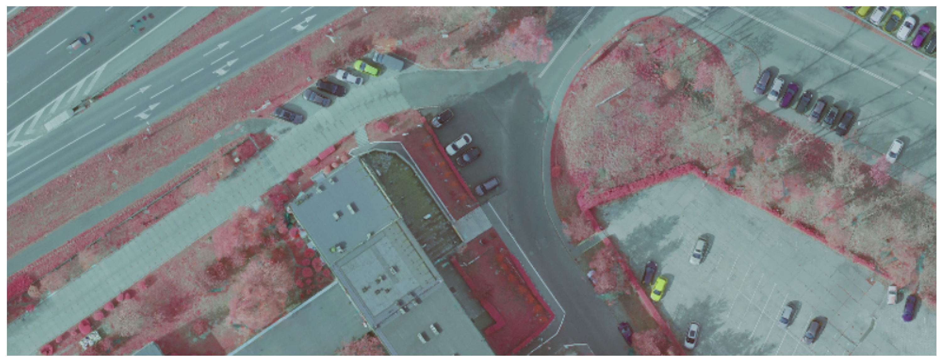
Color Infrared (CIR) remote sensing data, represented as normalized difference vegetation index (NDVI) images, offer insights into vegetation health through the contrast between the visible and near-infrared reflectance of plants. This method serves as a powerful, non-invasive tool for assessing vegetation. The data are stored in .tif format (TIFF), with each image corresponding to a specific map segment and including coordinate information. An example of a .tif file is illustrated in Figure 1, which differentiates between vegetation and urban structures using color intensity. For instance, a vivid red color signifies dense vegetation, while blue, gray, and yellow hues indicate areas with minimal or no vegetation.

GeoTIFF data encompass an urban area segmented into 562 zones, each measuring 500 by 800 m. This format serves as an open metadata standard that augments .tif files with georeferencing and geocoding data. Included in this added information are geographic coordinates, datum parameters, and mapping details, among others, which are instrumental in analyses such as vegetation index studies.

The final data format discussed is the world file for .tif files, which augments .tif files with additional information. Each corresponding .tfw file matches the coverage area of its .tif counterpart. Furthermore, .tfw files, in ASCII text format, provide rotation details and geographic coordinates for TIFF images.

An example of a file with a .tfw extension is illustrated in

Table 2. Example world file for a .tif file.

Structure of the .tfw File
0.05
0
0
−0.05
6569600.025
5559999.975

. This file complements the graphic NDVI files by containing additional metadata not present in the image itself, which indicate vegetation levels. In the example provided, the .tfw file comprises a series of lines that specify the X and Y pixel sizes, rotation information, and world coordinates for the upper-left corner of the image. In this case, the rotation value of the image is set to 0. However, this parameter becomes crucial when aligning aerial photographs with map overlays to accurately position the imaged area clusters.

Figure 2 shows the range of all data: the ground elevation above sea level, the height of buildings above sea level, the normalized difference vegetation index, and metadata .twf data.

3.2. Image-Processing Tools and Techniques

Image processing plays a vital role in automatically extracting objects from images. Several works have reported the application of this technique for urban area analysis, particularly focusing on green areas.

The essential tasks in such classification systems are image segmentation and object detection. In image segmentation, the main idea is to divide the original image into small, consistent fragments representing different objects and elements. Segmentation can be used to extract areas, including vegetation, buildings, roads, or other important elements of city architecture. The quality of the classification in the next steps of an algorithm depends on the size of the fragments and the quality of the image. An example of such segmentation can be seen in Figure 3, where the original image is divided into segments (the three black rectangles in the figure). In contrast, the first and second examples (“A” and “B” in the figure) show road and field fragments visible in the segment, while the last segment presents parts of the road and field occupying a similar space on the fragment.

The next problem that arises with these images is related to the quality of the image. Problems related to image quality may include the following:

• A low image resolution;
• Noise (artifacts) in the image.

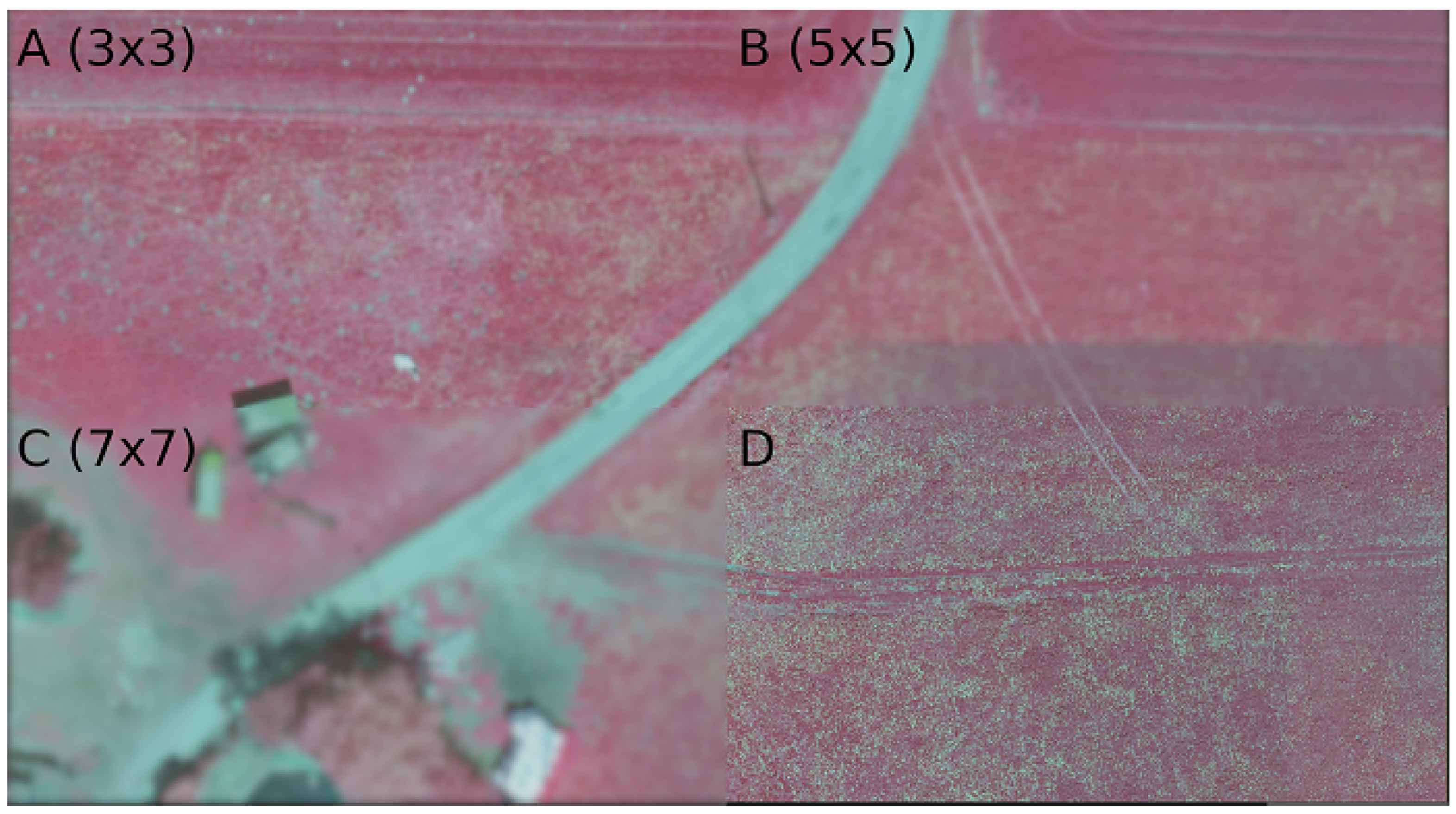
The resolution strictly depends on the availability of the data, and obtaining the same image in high resolution may not be possible. In contrast, image denoising can be performed using selected filters. Thus, the initial adjustment of filters (focusing on blurring filters) should positively affect the segments containing fragments of analyzed objects.

Image smoothing can be performed by convolving it with a Gaussian function representing a probability distribution over a continuous variable. It is characterized by two parameters: the mean and the variance. In addition, it represents the amount of blurring applied to each pixel in the image. The output of a Gaussian blur operation on an image can be represented mathematically as

$$G(x,y)={\displaystyle \frac{1}{2\pi {\sigma }^2}}·exp\left(-{\displaystyle \frac{x^2+y^2}{2{\sigma }^2}}\right)\ast I(x,y),$$

(1)

where $G(x,y)$ represents the blurred image, $I(x,y)$ represents the original image, $\sigma$ represents the standard deviation of the Gaussian function, and ∗ represents the convolution operator. Examples of Gaussian filters for different kernel sizes are presented in Figure 4.

Image segmentation and blurring are utilized to enhance the classification quality of image fragments. A decision class is assigned to every fragment of the map. For example, the average color of an image can be determined by calculating the mean values of the RGB (Red, Green, Blue) color channels for each pixel in the image [32].

Given an image I of size $M\times N$, the average color $\overline{C}$ can be computed as

$$\overline{C}={\displaystyle \frac{1}{M\times N}}\sum _{i=1}^M\sum _{j=1}^N[R_{i,j},G_{i,j},B_{i,j}],$$

(2)

where $R_{i,j}$, $G_{i,j}$, and $B_{i,j}$ denote the intensity values of the red, green, and blue channels, respectively, for the pixel at position $(i,j)$. The resulting vector $\overline{C}$ signifies the image’s average color across the channels. In our methodology, the dominant color is indicated by the maximum value among the calculated averages.

The quality of the classification can be assessed using classical classification metrics, such as precision, recall, or F1 score. However, it is important to note that in the case of maps, more than just numerical data acquired from the image may be required, and additional information from various sources may be necessary. An example of this and our proposed solution for vegetation and tree recognition on maps is the main focus of the system described in the next section.

4. Proposed Approach

Vegetation, particularly the location and arrangement of trees, plays a crucial role in spatial planning and sustainable development, especially in the context of green energy. Artificial intelligence and machine learning methods have become increasingly important in fields such as spatial planning. Therefore, the main goal of our proposed system is twofold: first, to automatically estimate the areas covered by high-vegetation plants and compare the results with maps obtained from the administration unit; and second, to assess the quality of classification in identifying trees on the maps using additional data from other map-related sources. High-vegetation areas predominantly consist of trees and fields. However, due to increased complexity, we have chosen to focus specifically on automatically recognizing trees on the maps.

The available TIFF maps indicating potential areas of high vegetation were not precise enough to allow for automated analysis. Therefore, we used additional elements related to the height above sea level. By incorporating this information, we can assign labels such as “tree”, “field”, “building”, and “road” to small map segments (each sized 1 square meter). In this section, we present a flowchart of our proposed system and provide details related to its implementation, along with a description of the algorithm. The proposed approach aims to achieve two main goals:

• Estimate the percentage of a given area covered by high-vegetation plants and verify the differences between the data held by the administration unit and the data resulting from our proposed algorithm.
• Verify the efficiency of the proposed approach in classifying map segments containing trees and compare the results with those obtained solely based on the maps derived by the administration unit.

The methodology proposed in this study uses data from multiple sensors, which collectively enable a comprehensive analysis of urban vegetation. Unlike many existing studies that primarily consist of RGB or LiDAR data [19,20,21], our approach integrates multi-source data to provide a more detailed understanding of vegetation characteristics. This integration not only improves the detection of individual trees but also identifies vegetation-covered terrain that is not wooded, offering a broader classification of green areas. Such detailed information is particularly valuable for urban decision makers, as it supports a holistic assessment of both wooded and non-wooded vegetation regions. By providing actionable insights, the proposed approach improves the operational efficiency of urban planning and facilitates informed decision-making processes aimed at sustainable city development.

4.1. Flowchart and System

In this subsection, we present a flowchart of the proposed system, which includes all the necessary steps to label each segment of a map. The entire system is divided into four distinct phases, each comprising several steps. It is important to note that the preferences of the decision maker are taken into account based on the thresholds related to the minimum color observed in the segment, denoted as $\overline{c}$, and the height threshold, denoted as $\overline{h}$. The flowchart is shown in Figure 5.

The first phase, marked in the figure as “a”, includes data acquisition. This phase primarily involves obtaining all necessary information in raw format and no further calculations are performed. However, it is important to note that the acquisition phase also includes data verification and the subsequent reporting of missing files. In the case of missing data, two main scenarios are identified:

• If the GeoTIFF (map and vegetation index) file is present while the numerical terrain files are missing, the system is capable of labeling the segment of the map based on the information acquired from the vegetation data.
• If the GeoTIFF file is missing while the numerical terrain files are present, the segment label is calculated based on the height and the threshold $\overline{h}$ set by the decision maker.

At least one of the above formats is required to complete the labeling process. Phases “b” and “c” in Figure 5 can be conducted simultaneously since two types of information are necessary at this stage. We determined that the height data could be processed relatively quickly, so in a sequential approach, phase “b” is executed before phase “c”. In phase b, information from two types of .asc files is collected, and data related to map coordinates are used to calculate the elevation relative to the sea level for the entire map. The number of values obtained in this phase corresponds to the number of small segments dividing the entire map. Information about the size of these segments is included in the .tfw files.

Phase “c” focuses on map segmentation and calculates the dominant color, based on the vegetation index acquired from the GeoTIFF files. After phases “b” and “c”, this information is integrated with the decision maker’s preferences, which is performed in phase “d”. A single map segment can be labeled as a “tree” under certain conditions:

• The segment is labeled as a tree if the dominant color is red (indicating a high vegetation index value)—this information is derived from phase “c”;
• The segment is labeled as a tree if the height difference ($h_{diff}$), determined in phase “d”, exceeds a specific threshold $\overline{h}$.

The combination of the above conditions results in labeling the selected segment as a “tree”. This process is repeated for every segment on the map under consideration. The details and implementation of the system are discussed in the following subsection.

4.2. Algorithm and Implementation

A custom-designed algorithm was developed to accurately detect vegetation in images. The approach was based on data acquisition, pre-processing, image analysis, and classification. Due to the fact that the original photos were not accessible, the vegetation index could not be computed, as the original infrared (IR) and visible images required for such computation were not available. Therefore, the approach relied solely on a single image. The input images gathered by the Municipal Office were color-coded using a simplified method to compute the vegetation index. With the computations already performed, the authors proposed a two-step approach. In the first step, the dominant color was identified using a 1-square-meter grid, called the Region of Interest (RoI). Then, the height difference was computed using two input .asc files—one for the absolute height of the ground level and the other for the actual height of objects within the RoI. The visualization comprised two factors: the outline color indicates the dominant color within the square, and the number inside represents the height difference.

The entire concept is presented in Algorithm 1. TIFF images are the raw input files containing information about the vegetation index derived by the administration unit. The second type of input data is stored in .asc files, which include information about the ground level and height above sea level for TIFF image segments. The sizes of these segments are stored in the geoinformation files (.tfw).

The proposed method is parameterized, allowing for the adjustment of selected parameters to improve the quality of the results. The key parameters and their values considered in the approach are as follows:

• Filtering method for TIFF images: Blurring filters for removing artifacts from images were considered. Thus, besides the Gaussian filter, other filters, like the median filter, may be considered.
• Kernel size for the filter: The kernel size is adjusted to control the blurring effect on the image. For tree-covered areas, the size of the kernel may be increased to achieve better results.
• Set of labels for image segments: Two sets of labels were considered. The first set includes trees, buildings, and fields, while the second, more classic approach, uses a binary set $\{tree,otherobject\}$.
• Thresholds for colors and heights: These thresholds are used to adjust the labeling of image segments.

Algorithm 1: Algorithm for the label assignment for the maps.

Thus, data files are initially loaded, and geoinformation, including the segment sizes on the maps $(x,y)$ in meters, is extracted. The TIFF image is divided into segments called regions of interest (RoIs) with equal sizes of x by y meters. Lines 10–16 of the algorithm present the main idea of our approach, where for every segment s in the image, S color channels are extracted, and the dominant color value $c_{dom}$ is calculated. Please note that the average color $c_{avg}$ was also considered; however, due to poor results, the authors decided to use $c_{dom}$ in the experiments. The color segment is determined by $c_{dom}$. The .asc files include height information for all considered segments. Thus, lines 13–15 estimate the height above sea level for every segment. The idea is to label segments considered fields (meadows), small trees, large trees, and buildings.

Thus, at this stage, labels for the segments can only be determined based on the dominant color for the segment, which is related to the vegetation index. High vegetation is marked as red. However, high-vegetation trees should be marked as red and also have a high value of the $h_{diff}$ parameter. The discrete labeling function is formulated as follows:

$$L(c_{dom},h_{diff})=\left\{\begin{array}{cc}Tree\hfill & \mathrm{if}{h}_{\mathit{diff}}>\overline{h}\mathit{AND}{c}_{\mathit{dom}}>\overline{c}\mathit{AND}{c}_{\mathit{dom}}=\mathit{red},\hfill \\ Other\hfill & \mathrm{otherwise}.\hfill \end{array}\right.$$

(3)

Please note that in the case of other objects, the extended labeling function is formulated as follows:

$$L(c_{dom},h_{diff})=\left\{\begin{array}{cc}Meadow\hfill & \mathrm{if}{h}_{\mathit{diff}}<\overline{h}\mathit{AND}{c}_{\mathit{dom}}>\overline{c}\mathit{AND}{c}_{\mathit{dom}}=\mathit{red},\hfill \\ Building\hfill & \mathrm{if}{h}_{\mathit{diff}}>\overline{h}\mathit{AND}{c}_{\mathit{dom}}>\overline{c}\mathit{AND}{c}_{\mathit{dom}}=\mathit{green},\hfill \\ Road\hfill & \mathrm{if}{h}_{\mathit{diff}}<\overline{h}\mathit{AND}{c}_{\mathit{dom}}>\overline{c}\mathit{AND}{c}_{\mathit{dom}}=\mathit{green},\hfill \\ Field\hfill & \mathrm{if}{h}_{\mathit{diff}}<\overline{h}\mathit{AND}{c}_{\mathit{dom}}>\overline{c}\mathit{AND}{c}_{\mathit{dom}}=\mathit{blue},\hfill \\ Other\hfill & \mathrm{otherwise}.\hfill \end{array}\right.$$

(4)

5. Numerical Experiments

This project involved the city of Katowice, which is 165 square kilometers. The location was divided into rectangular regions measuring 500 m by 800 m, resulting in a total of 562 regions. All data used in each region were saved as separate files (.asc and .tif). Our proposed approach was evaluated in selected regions of the city, encompassing various types of terrain.

All experiments were conducted on a Jupyter Notebook installed on a Vertex AI service provided by the Google Cloud Platform (GCP). The notebook was hosted on a virtual machine (named n1-standard-16 on GCP) with 16 vCPUs and 60 GB of RAM.

In the numerical experiments, we employed well-known measures, such as accuracy, precision, the Jaccard index, and the conformity index. The following classes were proposed:

• Tree—represented by red on the NDVI sample;
• Other objects—indicated by green or blue on the sample.

We assumed the following:

• High vegetation—red on the NDVI sample and a height of at least 15 m;
• Vegetation—red on the NDVI sample and a height of below 15 m;
• Other objects—green or blue on the NDVI sample.

By a single sample, we mean the smallest fragment on the map. The following assumptions were made:

• $TP$ (true positive)—sample considered a tree in both the original NDVI map and the result using our proposed algorithm;
• $TN$ (true negative)—sample not considered a tree in both the original NDVI map and the result using our proposed algorithm;
• $FP$ (false positive)—sample considered a tree in the original NDVI map but not recognized as high vegetation using our approach;
• $FN$ (false negative)—sample not considered a tree in the original NDVI map but eventually recognized as high vegetation using our approach.

The formulas for the aforementioned metrics are as follows:

$$ACC={\displaystyle \frac{TP+TN}{TP+FP+FN+TN}},$$

(5)

$$PREC={\displaystyle \frac{TP}{TP+FP}},$$

(6)

$$REC={\displaystyle \frac{TP}{TP+FN}}.$$

(7)

Since the occurrence of a situation in which a false negative (FN) greater than 0 was unlikely, we omitted this metric in our further calculations. Eventually, we selected accuracy and precision as the classification metrics. Further, we selected two different similarity metrics to estimate the dependence between the area indicated as vegetation (red on the map) and the height of the samples. These metrics are described as follows:

• Conformity index (CC), which is the relation between the TPs, FNs, and FPs:

  $$CC=(1-{\displaystyle \frac{FP+FN}{TP}})·100;$$

  (8)
  The interpretation of this metric is as follows: higher values indicate a better solution. Values below zero indicate a situation in which many samples initially assigned to the vegetation class were not considered trees after including the height data.
• Jaccard index, which indicates the similarity between two areas. In our case, we assume that A represents an area of vegetation, whereas B represents samples with a height greater than 15 m. Thus, the equation is expressed as follows:

  $$JI={\displaystyle \frac{A\cap B}{A\cup B}}.$$

  (9)
  In this case, values close to zero are better. However, the vast number of samples initially estimated to be vegetation (without including the height data) is expected to be omitted. Thus, this value should be closer to zero than to one.

5.1. Case Analysis

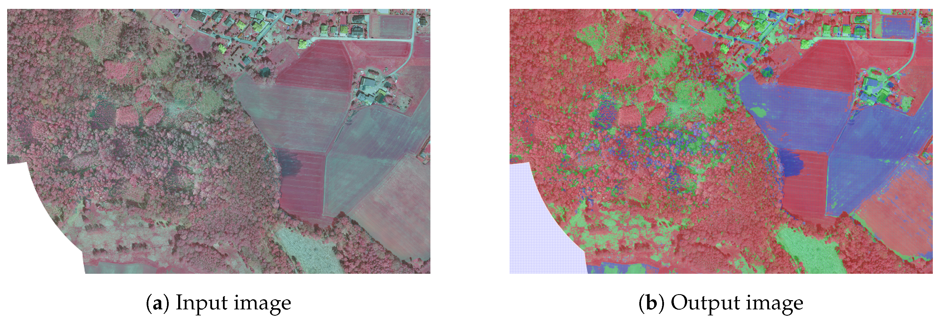
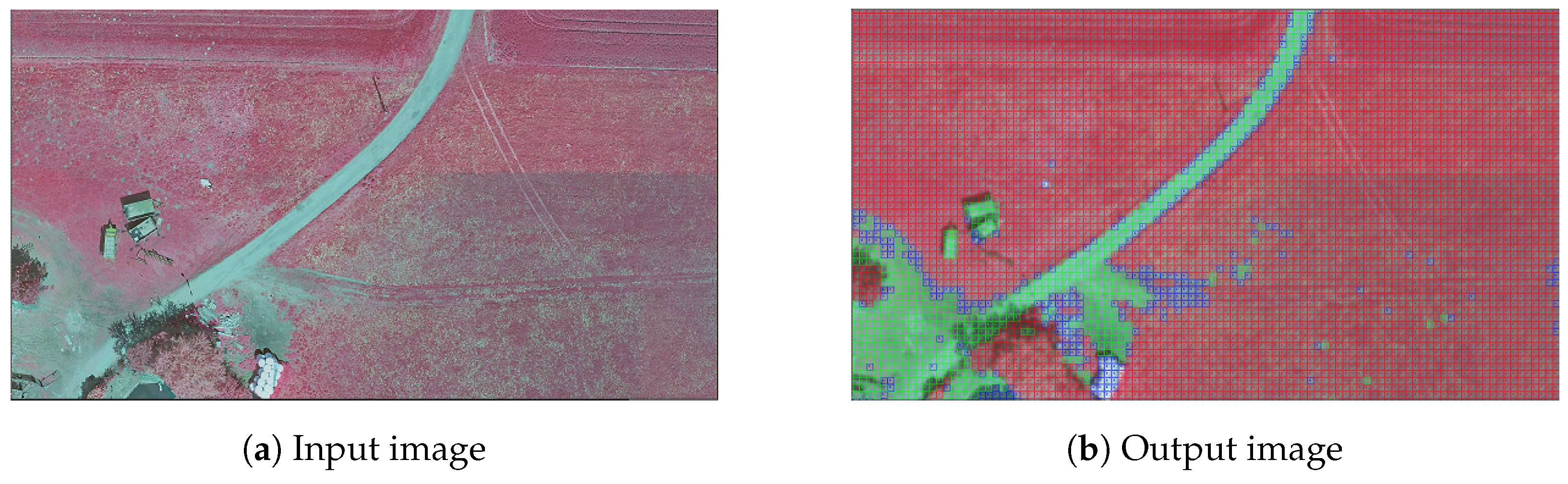
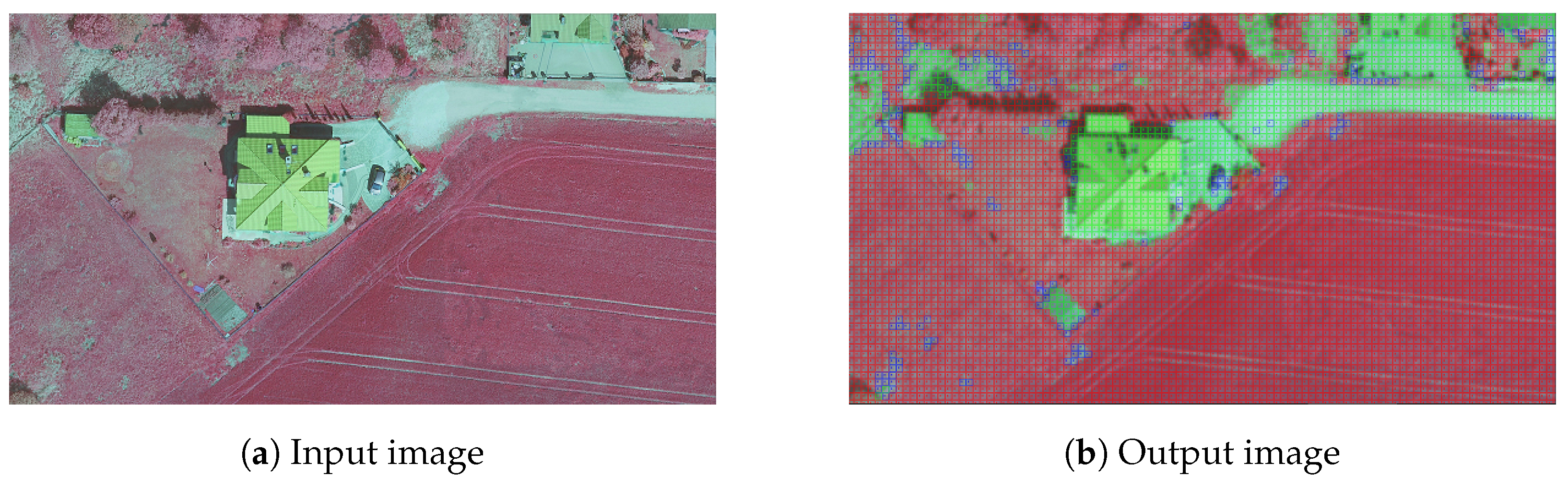
The outcome of the proposed approach is presented in Figure 6. The colors of vegetation and other areas are enhanced, while at the same time, the noise in different parts of the image is also reduced. This allows for better labeling of the whole area with vegetation without interference from shadows and other small artifacts. Furthermore, Figure 7 and Figure 8 show the details of two interesting areas. It can be seen that our approach correctly classified vegetation, both in open areas and in backyards. Details such as pavements or small structures were correctly color-coded, while individual trees and bushes were classified as vegetation. The algorithm also correctly classified a dirt track as non-vegetation.

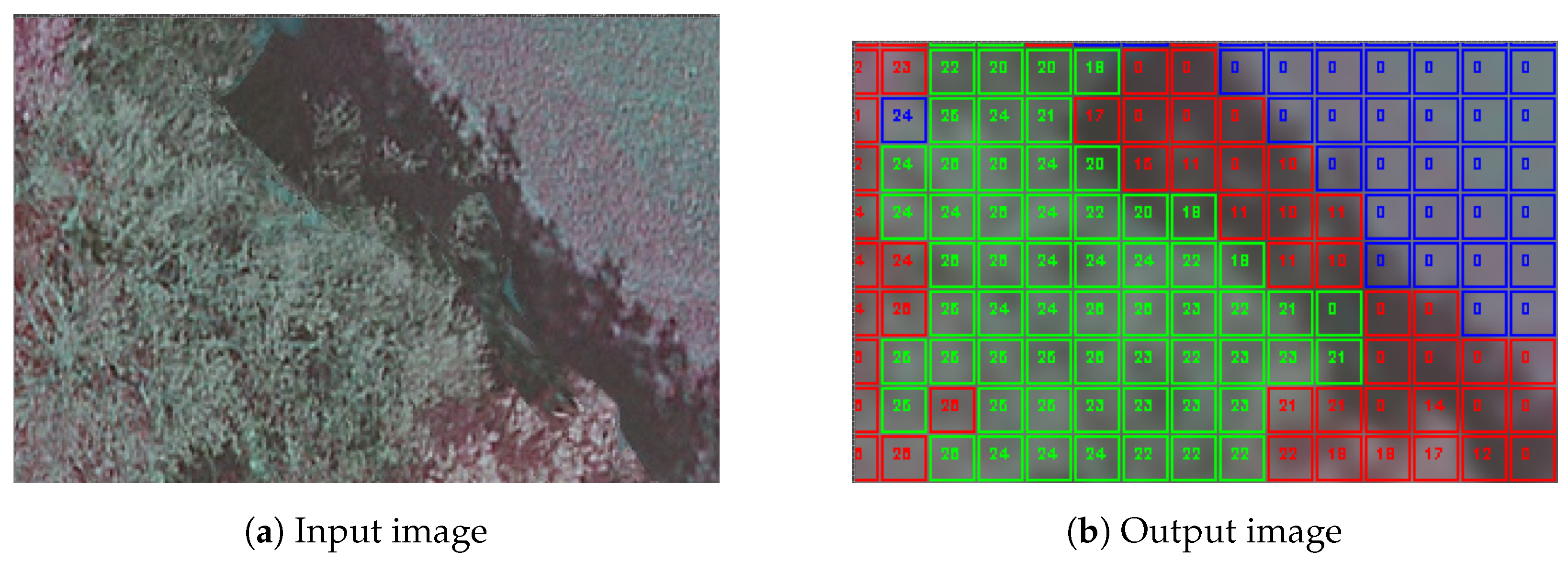
Figure 9 shows an example of a potential improvement. By incorporating information about the height difference, the edge-detection algorithm can be applied to further reduce noise in individual subareas by marking them in different colors from their surroundings.

5.2. Results

First, we analyzed and compared the percentage of the area covered by vegetation. However, we did not differentiate based on height information (see the first two columns on the left in

Table 3. The results for the percentage of the area covered by vegetation (the left part of the table) and the same information differentiated by high vegetation–trees, other vegetation, and remaining objects (like roads or buildings).

Dataset	NDVI Data		NDVI and .asc Data
	Vegetation	Other	High Veg.	Other Veg.	Other
6.127.29.03.1	60.5%	39.5%	27.7%	32.8%	39.5%
6.130.29.24.4	28.2%	71.8%	2.4%	25.8%	71.8%
6.130.29.24.2	47.4%	52.6%	5.9%	41.4%	52.7%
6.130.29.20.2	49.4%	50.6%	6.0%	43.4%	50.6%
6.130.29.14.4	43.5%	56.5%	18.4%	25.1%	56.5%
6.130.30.11.2	12.6%	87.4%	1.0%	11.6%	87.4%
6.129.30.17.1	60.5%	39.5%	35.8%	24.7%	39.5%
6.129.29.25.3	48.5%	51.5%	11.6%	36.9%	51.5%
6.129.29.14.3	71.2%	28.8%	0.0%	71.2%	28.8%
6.128.29.22.2	67.8%	32.2%	0.0%	67.8%	32.2%
6.128.29.20.3	76.9%	23.1%	22.5%	54.4%	23.1%
6.128.29.05.4	77.9%	22.1%	49.9%	27.9%	22.2%

). We can see that the vegetation area varies across different datasets, with the lowest value being 12.6% (the sixth row), and the highest value being 77.9% (the last row). Next, we incorporated height information to further differentiate the vegetation data separating trees (vegetation with a height difference from sea level over 15 m) from the remaining vegetation (like meadows). These data can be seen in the three columns on the right in Table 3. The most important observation here is the ”High veg.” column, which represents trees, and the ”Other veg.” column, which represents the remaining vegetation. Notably, the tree areas, which are crucial to our study, constitute only a small portion of the area initially marked as ”Vegetation” (the first column in Table 3). Thus, it can be assumed that the actual area of high vegetation around the city is much smaller, as indicated only by the NDVI data.

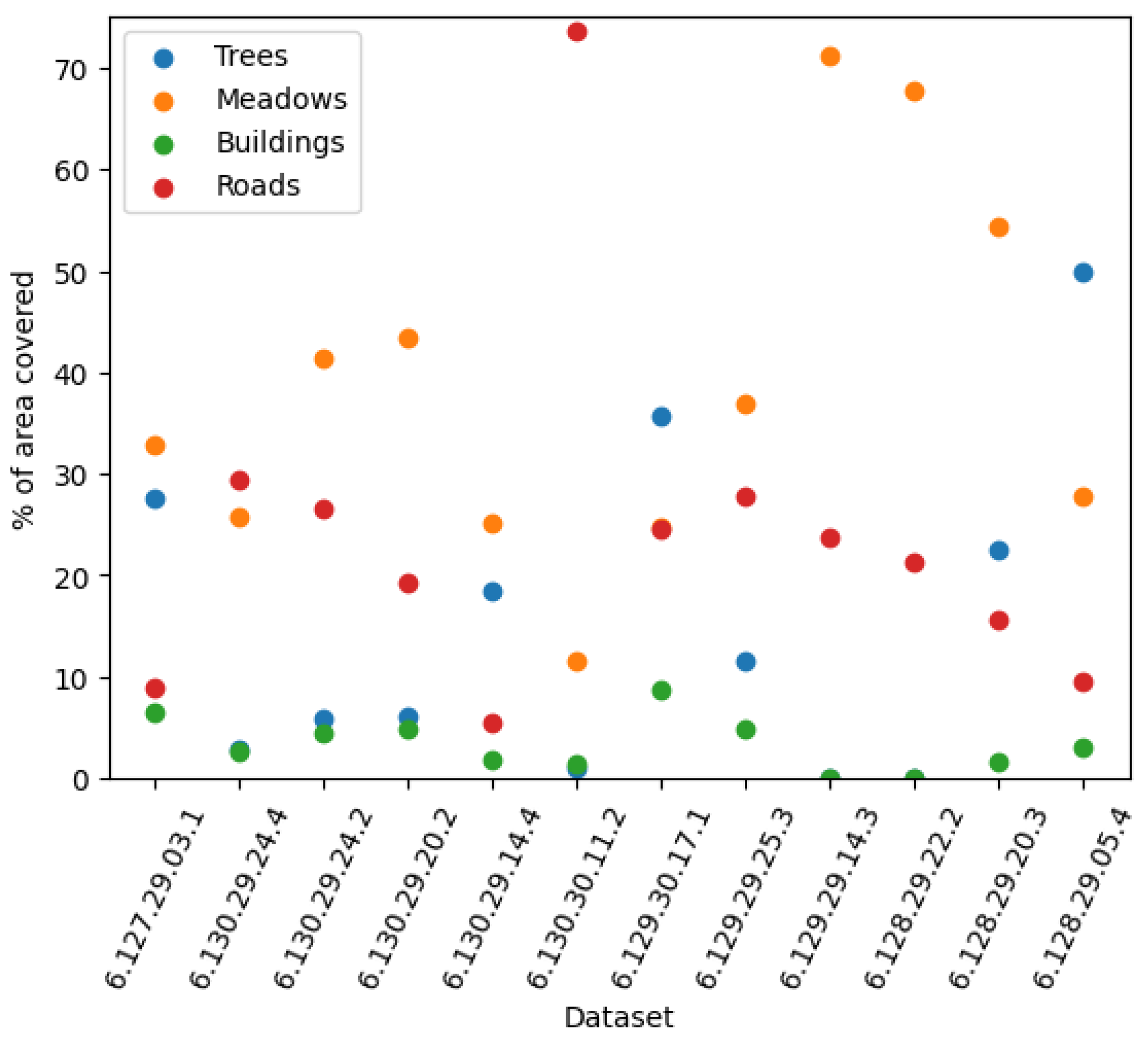
Next, we analyzed the percentage of objects other than vegetation in the available datasets. This information is presented in Figure 10, where we indicate the coverage of the area by various objects. Notably, the area covered by buildings (green dots in the figure) was relatively small in all cases, accounting for less than 10% of the area. There was considerable variation in road coverage, with three datasets covering only around 5% of the area, the second dataset including around 30% of roads, and the sixth dataset including over 70% of roads. The most important aspect of this analysis is the distinction between high vegetation (trees) and low vegetation (for example, meadows). Several datasets showed substantial differences between these two categories, while two datasets did not include any trees at all. Thus, it can be observed that the proposed approach is well suited for estimating the area coverage of various types of samples (trees, roads, or meadows). This information could be used directly to estimate areas where the coverage of high vegetation is expected to increase.

Ultimately, we were interested in the percentage of samples initially classified as vegetation (based on NDVI files) that, when height information from .asc data was considered, were not classified as trees. At the same time, we investigated the difference between two areas: one labeled as vegetation only and the other with a height greater than 15 m. Both results can be seen in

Table 4. Example comparison of color-based and color/height-based algorithms for selected datasets, focusing on overlapping and statistical metrics.

Dataset	Overlapping Metrics	Statistical Metrics
	Jaccard	CC	Accuracy	Precision
6.127.29.03.1	0.4219	−19.352	67.20%	45.80%
6.130.29.24.4	0.0795	−987.421	74.20%	8.40%
6.130.29.24.2	0.1199	−601.697	58.60%	12.50%
6.130.29.20.2	0.1099	−627.342	56.60%	12.10%
6.130.29.14.4	0.4181	−36.385	74.90%	42.30%
6.130.30.11.2	0.7055	−1085.412	88.38%	7.78%
6.129.30.17.1	0.5432	30.962	75.29%	59.16%
6.129.29.25.3	0.2333	−219.625	63.08%	23.83%
6.129.29.14.3	0.0000	∞	28.80%	0.00%
6.128.29.22.2	0.0000	∞	32.19%	0.00%
6.128.29.20.3	0.2895	−142.521	45.55%	29.20%
6.128.29.05.4	0.6245	44.007	72.05%	64.11%

. Two overlapping metrics (the Jaccard index and the conformity index) were used to estimate the difference between the two areas: the vegetation area based on NDVI data and the combination of NDVI data and height information. For the Jaccard index, the best value would be 1—indicating that all vegetation identified by the NDVI data is high vegetation—while a value of 0 would indicate the opposite—none of the identified areas are trees.

We can see that only in selected cases did trees cover more than 20% of the entire vegetation area, while the three remaining datasets showed relatively small coverage of trees. These results are confirmed by the CC index, which indicated that the large number of samples labeled as vegetation were not trees (lower values suggest a small number of trees in the area). Thus, we were able to identify areas in which, despite relatively high vegetation coverage (compare with the third, fourth, and eighth datasets in Table 3, where the vegetation coverage was around 47–49%), trees were lacking.

Similar conclusions can be drawn from statistical metrics like accuracy and precision, as shown in the last two columns of Table 4. Accuracy and precision focus on deriving the information that represents the percentage of areas initially marked as vegetation that did not include trees.

6. Conclusions

In this study, we developed an automatic method for detecting and evaluating trees in urban environments using image-processing and data integration techniques. By combining various data sources, including maps, vegetation indices, and numerical land data, we successfully identified and mapped trees within the city of Katowice, Poland. Our approach not only improves the efficiency of urban tree management processes but also supports sustainable urban development by providing accurate and up-to-date information on vegetation coverage.

The results demonstrated that our method could effectively identify areas that are assumed to have a high vegetation cover but are actually lacking sufficient tree density. This information is crucial for urban planners and decision makers who want to expand green spaces and improve ecological balance within urban settings. Additionally, our methodology can be extended to label other objects on maps, such as buildings or roads, by integrating additional data sources.

Automatic detection and assessment of trees and wooded areas are essential steps toward intelligent urban environment management. Using modern technologies such as image analysis, machine learning, and geospatial data processing can significantly accelerate and improve the monitoring, assessment, and protection of urban vegetation. This contributes to creating greener, more resident-friendly cities, enhancing the quality of life, protecting biodiversity, and mitigating the adverse effects of climate change.

Future work could involve applying this method to other urban areas, integrating additional data sources such as hyperspectral imagery, or refining algorithms to further improve detection accuracy. By continuing to develop and implement these innovative technologies, we can contribute to the construction of more sustainable and environmentally friendly urban spaces, ultimately preserving valuable ecosystems for future generations.