Abstract
Background: This paper aims to complement the latest contribution in the literature that provides estimates of physiological parameters of a dynamic model for the elbow time profile during walking while linking them to a neurodegenerative disorder (Parkinsons’s disease) characterized by motor symptoms. An upper limb model is here proposed in which an active contractile element is included within a model, viewing the arm as a double pendulum system and muscles as represented by a Kelvin–Voight system. All model parameters characterizing both the shoulder and the elbow of each subject are estimated via a gradient-like identifier whose exponential convergence properties are determined by a non-anticipative Lyapunov function, ensuring robustness features. Methods: Joint angle data from different walking subjects (healthy subjects and patients with Parkinson’s disease) have been recorded using an IMU sensor system and compared with the joint angles obtained by means of the proposed model, which was adapted to each subject using available anthropometric knowledge and relying on the estimated parameters. Results: Experiments show that the reconstruction of shoulder and elbow time profiles can be definitely achieved through the proposed procedure with the estimated stiffness parameters turning out to constitute objective and quantitative indices of muscle stiffness (as a pivotal symptom of the pathology), which are able to track changes due to the therapy. Conclusions: The same dynamic model is actually able to capture the main features of the upper limb movement of both (healthy and pathological) walking subjects, with its parameters, in turn, characterizing the nature and progress of the pathology.
1. Introduction
A fundamental aspect of walking is represented by the arm movement. Many studies have been conducted to characterize it [1,2,3,4,5,6], though several aspects are yet to be clarified. For instance, arm movement seems to have a positive effect on an individual’s stability [2] while minimizing the energy cost of walking. Regarding the source of such movement, researchers have tried to verify the hypothesis that the arms behave like passive elements that move in response to the movements of the torso and of the shoulders [3], thus acting as pure dampers. On the other hand, EMG activity—in the muscles responsible for arm movement—has been actually found during walking at a pace of about 4 km/h, though it is much reduced with respect to the maximum voluntary muscle contraction [4,5]. This seems to suggest that arm movement also involves an active component: realistic movement cannot be achieved [6] in the absence of active components.
In order to study the kinematics and the dynamics of human walking, a mathematical model is generally used, which relies on coefficients owning a physical meaning while directly allowing for simulations of different test conditions. In this regard, several models have been proposed over the years, depending on the type of the considered body movement. For example, the detailed kinematic analysis of Petković and associates [7] provides valuable insights into gymnasts’ techniques; a model with 37 degrees of freedom based on a Hill muscle model has been proposed by Rajagopal and associates [8], which is capable of simulating the kinematics of the lower limbs during walking; a similar approach has been followed by Cardona and associates [9] for modeling the behavior of lower limbs in a medical context, which involves healthy subjects and subjects with disorders such as stroke or heart attack.
As far as upper limbs are concerned, researchers in the literature have mainly focused on complex movements like reaching and manipulating a target. This is rather useful for robot control design [10,11,12]. Models have been proposed even to reproduce the role of the upper limbs during walking. For example, the upper limbs have been modeled by Pontzer and associates [3] as a system of springs and masses, reacting to lower body movements. A simple pendulum has been used by Gutnik and associates [13] to describe its movement, resulting in an estimated angular velocity smaller than the actual one, which is probably because an active term representing muscle activity was not considered as well. On the other hand, the limb has been also modeled as a double pendulum with a constraint representing the elbow [14,15]. Realistic results have been obtained for different step cadences, though the accuracy of the model regarding a specific subject suffers from the use of parameter values that are averaged over a population.
In this paper, which improves our previous work [16]—restricted to provide estimates of the parameters characterizing the dynamics of the elbow only without furnishing a model-based recostruction of the joint angles—a more complex upper limb model for walking is proposed. The arm is still modeled as a double pendulum system, whereas muscles are still represented by a Kelvin–Voight model, with the passive element, instead, now appearing in parallel to a newly introduced contractile element. Nevertheless, all the model parameters characterizing the shoulder and elbow movement of each specific subject—differently from papers [14,15]—are identified through a gradient-like identifier—other than the least square used by Pietrosanti and associates [16] and relying on a single gait—whose exponential convergence properties are ruled by a non-anticipative Lyapunov function [17]. The effectiveness of the proposed method is illustrated by experimental results. Joint angle data from different walking subjects have been recorded using an IMU sensor system and compared with the joint angles obtained by means of the proposed model, which was adapted to each subject using available anthropometric knowledge and relying on the estimated parameters. Furthermore, to validate the use of the proposed approach for diagnostic purposes, the same procedure has been repeated with reference to a cohort of subjects with Parkinson’s disease (PD) [18,19,20], and the estimated stiffness parameters (meaningfully concerning both the shoulder and the elbow for a better movement characterization) have been used as objective quantitative indices of muscle stiffness. Indeed, the results of this paper, as for [21], show how the same dynamic model might capture the main features of the upper limb movement of walking subjects, whereas its parameters characterize the progress of the (PD) pathology. In this regard, PD is a neurodegenerative disorder characterized by motor and non-motor symptoms [18]. The cardinal motor symptoms are rest tremors of limb extremities, muscle rigidity [19], bradykinesia, i.e., slowness in movements, and gait instability. It is well known that PD strongly affects gait, causing instability and an altered range of motion [20]. This specific neurologic condition has been chosen because muscle stiffness is a cardinal symptom of the disease, and one of the challenges in this field of research is to find a method for measuring it since, to date, there is no validated method—beyond the (almost subjective) Movement Disorder Society Unified Parkinson’s Disease Rating Scale (MDS-UPDRS) [22]—that is capable of quantifying this symptom over a compact subset of the set of real numbers [23,24,25]. In this light, the paper moves, though within a different context, along the direction of [26]. It aims to complement the latest contribution in the literature that provides estimates of physiological parameters of a dynamic model for the elbow time profile during walking while linking them to the action of the Parkinsons’s disease.
2. Materials and Methods
2.1. Subjects
For model validation, a group of 4 healthy subjects (namely, HS1–HS4) and 3 patients with PD (namely, P1–P3), enlisted from the Movement Disorders Outpatient Service of Sapienza University in Rome, Italy, was recruited. The clinical evaluation of patients with PD involved assessing MDS-UPDRS scores, focusing on primary motor symptoms such as bradykinesia, rigidity, tremor, gait, and balance issues. Cognitive functions were evaluated using the Mini-Mental State Evaluation (MMSE) [27], which is a comprehensive cognitive scale assessing various abilities including orientation, memory, fluency, attention, and visuospatial skills. Moreover, the Hoehn and Yahr scale [28], Beck Depression Inventory-II (BDI-II) [29] and Parkinson’s Disease Questionnaire (PDQ-39) [30] were included in patients’ assessment. Inclusion criteria for patients with PD included a diagnosis of idiopathic PD according to consensus criteria, H&Y scale ≤ 2.5, and the ability to keep up the right stance and walk independently. Exclusion criteria comprised diagnosis of atypical parkinsonism, severe PD (H&Y > 2.5), L-Dopa-induced dyskinesia, dementia (MMSE < 24), and comorbidities affecting gait or arm movements (e.g., orthopedic, or rheumatologic issues, polyneuropathies, and other neurological disorders).
Patients with PD were undergoing chronic dopaminergic treatment. Arm swing during gait, akin to rigidity, bradykinesia, or tremor, may benefit from levodopa intake. Therefore, PD patients were evaluated in two sessions according to the therapeutic condition: the OFF (i.e., after drug withdrawal for at least 12 h) and ON state of therapy (i.e., one hour after taking the 150% of their usual L-Dopa dose). The L-Dopa equivalent daily dose (LEDD) was calculated according to standardized procedures [31]. Anthropometric data (weight, height, center of mass, and turning radius for both upper arm and forearm) were used to allow for detailed modeling. Table 1 and Table 2 summarize participants’ demographic and clinical features.

Table 1.
Demographic and clinical features of participants. H&Y: Hoehn and Yahr scale; DD: disease duration.
Table 2.
Demographic and clinical features of participants. BDI-II: Beck Depression Inventory-II; SC stands for MDS-UPDRS: Movement Disorder Society Unified Parkinson’s Disease Rating Scale; MMSE: Mini-Mental State Evaluation; PDQ-39: Parkinson’s Disease Questionnaire.
2.2. Hardware
To record kinematic features from gait, we adopted the—already validated and most reliable for our purposes [32]—network of 13 lightweight (48 mm × 39 mm × 18 mm, 27 g) wearable inertial sensor units (IMUs) belonging to the Movit System G1 (by Captiks) in Figure 1 (left). Each unit mounts a tri-axial accelerometer (±16 g, 16 bit resolution, 2048 LSB/g sensitivity, 200 Hz sample rate), tri-axial gyroscope (±2000 deg/s, 16 bit resolution, 16.4 LSB/dps sensitivity, 200 Hz sample rate), and tri-axial magnetometer (±4800 T, 16 bit resolution, 0.6 T/LSB sensitivity, 200 Hz sample rate). The devices were placed directly on the subject’s body by means of non-invasive Velcro straps in order to preserve proper mobility. In Figure 1 (right), the position of each sensor on the body is depicted. Recorded data were sent to a pc by means of wireless communication (2.4 GHz—based on IEEE 802.15.4 MAC [33]), whereas a dedicated software named MotionStudio 3d (version 2.5.3) allows us to rule the recording process. Raw data collected from the accelerometer, gyroscope, and magnetometer were analyzed by means of the dedicated software MotionAnalyzer (version 1.4.2) in order to compute joint angles.
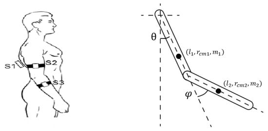
Figure 1.
(Left) Configuration of the Movit System Units on the participant’s body. (Right) Graphical representation of the double pendulum system.
2.3. Test Protocol
Healthy subjects were asked to walk for 10 m. Each subject performed three different trials at different predefined paces of 80, 100, and 120 step/min. To help participants, an electronic metronome was used to give acoustic feedback. Moreover, each subject could repeat the test until they felt totally confident with the cadence. PD subjects, instead, were asked to walk at a comfortable speed for 10 m for the MDS-UPDRS test protocol.
2.4. Mathematical Model
We start from the model proposed by Jackson and associates [14]. The arm is represented as a double pendulum as shown in Figure 1 (right) with being the shoulder angle and being the elbow angle.
Indeed, the model relies on the Euler–Lagrange equations, which involve the Lagrangian function as the sum of the total kinetic energy and the total potential energy of the double pendulum. In the following formulas, (i) the subscripts 1 and 2 will refer to the upper link and lower link, respectively, whereas (ii) L represents the length of the segment, m its mass, the position of the center of mass, and I the moment of inertia. Anthropometric quantities are taken, for each subject, according to the related tables [34]. Furthermore, normalized and depend on the force applied by the shoulder muscles and the elbow muscles, respectively (CE stands for contractile element). On the other hand, depends on the force due to the linear acceleration of the shoulder, whereas depends on the force due to the acceleration of the elbow (a stands for the acceleration of the center of mass, coming from the IMU sensor system). Finally, , , , and represent the elastic constant, viscous constant, resting position, and CE of the shoulder, respectively, whereas , , , and denote the same parameters for the elbow, respectively. In fact, it is known that biological tissues, like muscles, present a viscoelastic behavior [35] with several models having been proposed over the years [36,37] to reproduce the muscle response. Indeed, a classical Kelvin–Voight model of viscoelastic materials is also adopted hereafter to model the viscoelastic properties of the muscles, as illustrated by Figure 2.
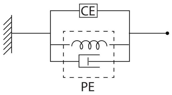
Figure 2.
Kelvin–Voight model for a viscoelastic material. CE stands for contractile element. PE is the passive element. The CE element represents the contractile behavior of the muscle in response to EMG activity, while the PE considers the elastic and viscous stiffness of muscle fibers, respectively, which are characterized by elastic constant and viscous constant (refer to , and , in model (1)–(5)).
On the other hand, a source of non-conservative force in the upper limb is the elbow constraint, which forbids a complete extension of the forearm, while a forward flexion is free ( is the position of the elbow at rest). As a matter of fact, the resulting model reads (dependence of state variables on time t is omitted for the sake of simplicity):
in which
is invertible for any , while
whereas
is the regressor matrix, thus multiplying the vector of unknown constant parameters:
2.5. Parameter Identification and Model Simulation
Define y as the column (bi-dimensional) vector whose components are the measured variables and . According to the model shown in Equations (1)–(5), the estimate of y, which is instrumental to obtain a converging estimate (with components , ) of , is defined as
Now, due to the absence of any EMG activity information for upper limb muscles, muscle torques cannot be measured in of (6). Consequently, according to well-known findings that indicate impulsive EMG activity for upper limb muscles during walking gaits, muscle torques are approximately set equal to the truncated Fourier series (up to the fifth order) of impulsive test signals with the same frequency of arm oscillation and 10% duty cycle (since no information about the time instants when the signal occurs is available, the parameter estimation algorithm and simulation runs are repeated twelve times by considering different uniformly distributed delays within 0 and : delays that lead to the most satisfactory set of Mean Squared Error (MSE), Root Mean Squared Error (RMSE), and Mean Absolute Error (MAE) are definitely selected for each subject) [see Figure 3] and assumed to approximately match and .
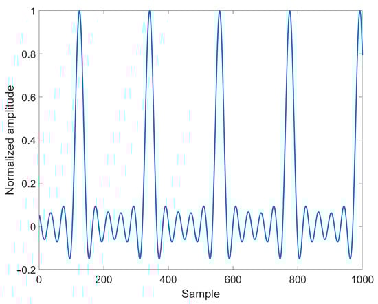
Figure 3.
Normalized test signal for approximating and .
Assume that and are perfectly matched. Then, the estimation error from (1) and (6) satisfies
in terms of . The -identifier is consequently designed as ( is a symmetric positive definite matrix)
which gives
The error system thus complies with the one studied by Verrelli and associates [17]. Exponential convergence to zero of —and thus robustness, along with exponential convergence to zero of —is proved under the persistency of excitation of the regressor that is related to an identifiability property [typical angle profiles and muscle forces filling the regressor (see the figures below) characterize the persistency of excitation] via the non-anticipative Lyapunov function proposed by Verrelli and associates [17]. In particular, the related Theorem 1 of paper [17], reported here for the sake of exhaustivity, reads
Theorem 1
([17]). Consider system
under the following assumptions: (i) is a symmetric positive definite constant matrix belonging to the set of real square matrices with n rows and n columns; (ii) the regressor matrix is available, continuous, uniformly bounded over (with norm-bound ) and persistently exciting (i.e., there exist (known) positive reals and such that the condition [ is the identity matrix]
holds); (iii) the smooth vector function R — uniformly bounded in t over for any bounded and over — is such that
in terms of suitable positive reals , , and , belonging to the set of functions satisfying
(iv) is a sufficiently small disturbance vector (possibly converging to zero for t tending to ). Its state vector (i) is locally ultimately bounded by a bound proportional to the (sufficiently small) upper bound on the -perturbation term; (ii) locally exponentially converges to zero for exponentially tending to 0. The related (strict) quadratic Lyapunov function reads
where is the solution to the matrix-differential equation
involving the symmetric positive definite matrix (with sufficiently large minimum eigenvalue) and the positive real ; is a sufficiently large positive real; is the signum function satisfying for , for .
The previous theorem shows that even in the case in which and are not perfectly matched, ultimate boundedness might be achieved in terms of a bound proportional to the signal mismatch. Now, to improve parameter convergence over a finite time horizon, the estimation process is carried out twice, and initial conditions for the estimates at the second run are set equal to the values obtained at the end of the first run (zero initial values for the estimates of the 3rd, 4th, 7th, 8th components of and for the other ones are chosen at the beginning of the first run). Finally, the gain matrix is set equal to for HS1–HS4 and to for P1–P3.
Estimated parameters are then employed for model simulation, and joint angles are computed by solving the related differential equations of the model through the explicit Runge–Kutta integration method. Joint shoulder and elbow angles coming from simulations are then compared to those measured by IMUs; MSE, and RMSE and MAE are then computed to quantify discrepancies between real and simulated data while assessing the ability of the identified model to reproduce the real movement.
3. Results
First, the results in reconstructing joint angle profiles through the model (with the estimated parameters) for the healthy subjects HS1–HS4 (for 100 bpm step cadence) and the PD patients P1–P3 (ON-OFF, at comfortable speed) are illustratively shown in Figure 4, Figure 5, Figure 6, Figure 7 and Figure 8, Figure 9, Figure 10, Figure 11, Figure 12, Figure 13, respectively [measurements concerning patient P1 underwent major calibration issues leading to unmodeled disturbances that affect both the parameter estimation and the recostruction of joint angles]. The harmonic content of real and simulated signals is also reported in Figure 4, Figure 5, Figure 6, Figure 7, Figure 8, Figure 9, Figure 10, Figure 11, Figure 12 and Figure 13. The MSE, RMSE, MAE values and the estimated model parameters are reported in Table 3, Table 4, Table 5 and Table 6. More in detail, Table 3 and Table 5 collect the resulting MSE, RMSE, and MAE values corresponding to the shoulder and elbow joints for both the healthy subjects and the patients with PD. On the other hand, Table 4 collects the estimates of parameters , for the healthy subjects HS1–HS4, all of them at three different speeds, namely, 80 steps/min, 100 steps/min and 120 steps/min. Finally, Table 6 contains the estimates of the stiffness parameters , , and for PD patients (walking at their comfortable speed), both for ON and OFF, aside from the MDS-UPDRS item 3.3 score (0: normal (no rigidity); 1: slight rigidity; 2: mild rigidity; 3: moderate rigidity; 4: severe rigidity).
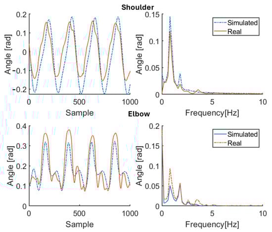
Figure 4.
Simulation results for healthy subject HS1 for 100 bpm step cadence. Red solid line: joint angle of shoulder and elbow. Blue dashed line: simulated angle of shoulder and elbow. Left: time domain. Right: frequency domain.
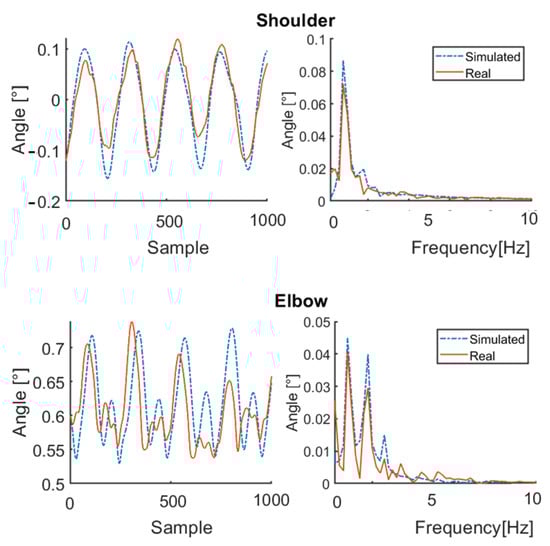
Figure 5.
Simulation results for healthy subject HS2 for 100 bpm step cadence. Red solid line: joint angle of shoulder and elbow. Blue dashed line: simulated angle of shoulder and elbow. Left: time domain. Right: frequency domain.
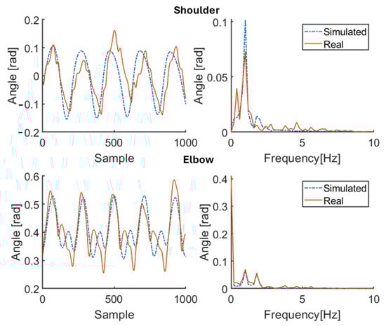
Figure 6.
Simulation results for healthy subject HS3 for 100 bpm step cadence. Red solid line: joint angle of shoulder and elbow. Blue dashed line: simulated angle of shoulder and elbow. Left: time domain. Right: frequency domain.
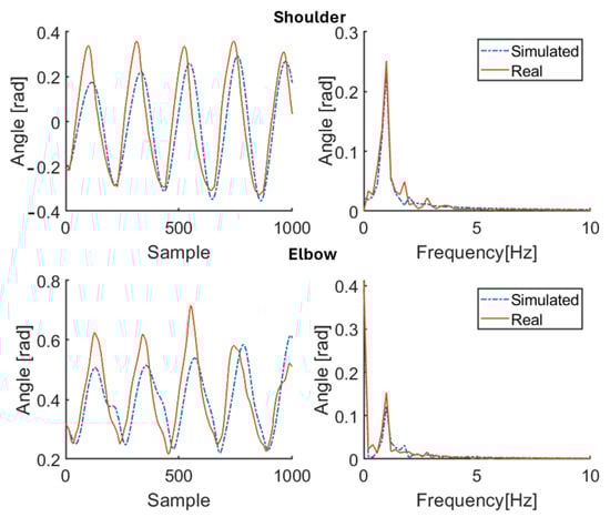
Figure 7.
Simulation results for healthy subject HS4 for 100 bpm step cadence. Red solid line: joint angle of shoulder and elbow. Blue dashed line: simulated angle of shoulder and elbow. Left: time domain. Right: frequency domain.
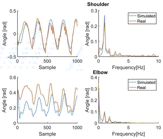
Figure 8.
Simulation results for patient P1 (therapy OFF). Red solid line: joint angle of shoulder and elbow. Blue dashed line: simulated angle of shoulder and elbow. Left: time domain. Right: frequency domain.
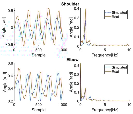
Figure 9.
Simulation results for patient P1 (therapy ON). Red solid line: joint angle of shoulder and elbow. Blue dashed line: simulated angle of shoulder and elbow. Left: time domain. Right: frequency domain.
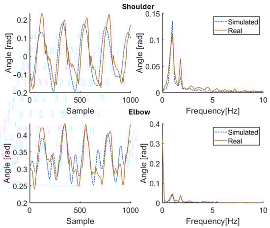
Figure 10.
Simulation results for patient P2 (therapy OFF). Red solid line: joint angle of shoulder and elbow. Blue dashed line: simulated angle of shoulder and elbow. Left: time domain. Right: frequency domain.
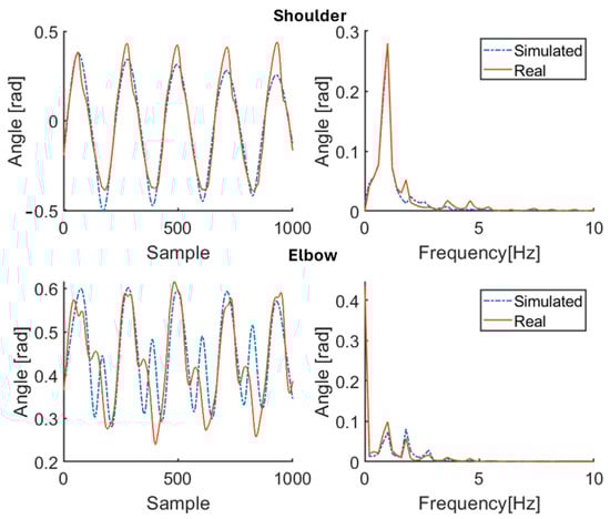
Figure 11.
Simulation results for patient P2 (therapy ON). Red solid line: joint angle of shoulder and elbow. Blue dashed line: simulated angle of shoulder and elbow. Left: time domain. Right: frequency domain.
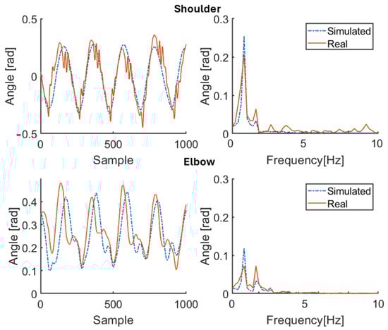
Figure 12.
Simulation results for patient P3 (therapy OFF). Red solid line: joint angle of shoulder and elbow. Blue dashed line: simulated angle of shoulder and elbow. Left: time domain. Right: frequency domain.
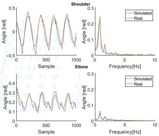
Figure 13.
Simulation results for patient P3 (therapy ON). Red solid line: joint angle of shoulder and elbow. Blue dashed line: simulated angle of shoulder and elbow. Left: time domain. Right: frequency domain.
Table 3.
Reconstruction errors for healthy subjects (at three different speeds).
Table 4.
Estimated parameters for healthy subjects (at three different speeds).
Table 5.
Reconstruction errors for patients with PD (ON and OFF, at comfortable speed).
Table 6.
Estimated stiffness parameters for patients with PD (ON and OFF, at comfortable speed) and MDS-UPDRS item 3.3 score.
4. Discussion and Limitations
The primary purpose of this study was to capture the main features of the upper limb movement of walking subjects (both the healthy and the pathological ones) while estimating all model parameters that characterize the shoulder and elbow movement. The secondary purpose was to use, for PD patients, the estimated stiffness parameters as objective quantitative indices of muscle stiffness in response to pharmacological therapy. The results confirm the effectiveness of the approach through a model whose structure is the same for both the healthy subjects and the patients and with the estimated stiffness coefficients tracking the effects of taking therapy in accordance with the MDS-UPDRS scores. In particular, the measured joint angles are properly reproduced by means of the proposed model once it is adapted to each subject using the available (specific) anthropometric knowledge and the physically consistent parameter estimates. Indeed, from Table 3 and Table 5, the values of MSE RMSE, and MAE for each subject are kept significantly small by the proposed procedure, showing its effectiveness in spite of the just approximated nature of the test signals reconstructing and . Values are lower for the shoulder than the elbow, owing to the hard-to-model stronger nonlinearities characterizing the latter. Moreover, Figure 4, Figure 5, Figure 6, Figure 7, Figure 8, Figure 9, Figure 10, Figure 11, Figure 12 and Figure 13 illustrate how the spectral content of recorded movements is satisfactorily reproduced, which was already evidenced to contain information related to a pathological condition [38]. The obtained results in terms of minimum errors are of crucial importance, since they demonstrate the capability to reproduce both healthy and pathological behaviors with the same model. On the other hand, Table 4 and Table 6 show how the estimates of the stiffness parameters . Values are lower for the shoulder than the elbow, owing to the hard-to-model stronger nonlinearities characterizing the latter. Moreover, Figure 4, Figure 5, Figure 6, Figure 7, Figure 8, Figure 9, Figure 10, Figure 11, Figure 12 and Figure 13 illustrate how the spectral content of recorded movements is satisfactorily reproduced, which was already evidenced to contain information related to a pathological condition [38]. The obtained results in terms of minimum errors are of crucial importance, since they demonstrate the capability to reproduce both healthy and pathological behaviors with the same model. On the other hand, Table 4 and Table 6 show how the estimates of the stiffness parameters , , and are actually negative, as physically expected for elastic and viscous constants. The same happens for the estimates of and , which are associated with muscle contraction: positive values are associated with arm flexor muscle activity, negative values are associated with extensor muscle contraction (the estimates of and depend, instead, on the balance position of the limb, while and characterize the amplitude of the active contribution). Arm oscillations are not discussed at this stage.
Table 4 illustrates how the estimated parameters for healthy subjects reasonably vary in accordance with the step cadence [35] (it is worth highlighting that subjects underwent difficulties in maintaining the slow cadence of 80 steps per minute and the fast cadence of 120 steps per minute). In contrast, Table 6, which reports the estimated stiffness parameters for patients with PD before — OFF state — and after therapy — ON state — (the estimates of the parameters obtained for the ON estimation procedure are used as initial conditions for the OFF estimation procedure to verify how the OFF status varies starting from the ON status) and the corresponding MDS-UPDRS item 3.3 scores related to stiffness (one of the pivotal symptoms for PD), illustrates the following: (i) the estimated stiffness coefficients approximately tend to decrease (increase in absolute value) after taking therapy, which is in accordance with MDS-UPDRS scores [coefficients closer to zero corresponds to lower stiffness]; (ii) subjects characterized by an MDS-UPDRS score different from zero have estimated stiffness coefficients higher with respect to the HS group, while those with a score equal to zero are characterized by estimated coefficients more in line with healthy subjects; (iii) even though there is no direct correspondence between MDS-UPDRS scores and estimated stiffness values, there is a correspondence in their variations; indeed, subjects transitioning from a score of 1 (rigidity only detected with activation manoeuvre) to 0 (no rigidity) exhibit a smaller change in estimated parameters (especially at the level of the elbow).
It is worth noticing that in contrast to our previous work [16], whose aim was just to quantify muscle rigidity at the elbow level in patients with PD, a more comprehensive analysis of human gait is presented in this paper with the role of whole arm movement within it being highlighted: sustained arm oscillations involve a combined action of an active term, muscle activity, and a passive term, with the proposed active component shape, at comfortable walking speeds, reproducing the behavior of the muscles that primarily serve to initiate the movement rather than to maintain it continuously. Indeed, the modifications of the estimated stiffness parameters in response to pharmacological therapy might shed more light on the relationship between motor and musculoskeletal biomechanical control in generating the movement of body segments. Finally, the closed-loop estimation method allows us to validate the model by comparing simulated joint profiles with measured ones without restrictions to averaged populations.
Some limitations can be drawn as well. Further research is in fact needed to enhance this study. For example, expanding the patient cohort and including individuals at various stages of PD, encompassing diverse phenotypes, disease durations, and clinical characteristics, would allow for a more comprehensive assessment of the robustness of the proposed approach across different stages and etiologies. Validating the model in distinct PD cohorts, such as those with early-onset Parkinson’s disease (EOPD) [39] or genetically driven forms of PD [40], could further reinforce its reliability and generalizability.
5. Conclusions
The dynamic model (1)–(5) has been used to capture the main features of the upper limb movement of walking subjects. All model parameters characterizing the shoulder and elbow movement of each subject have been identified through the gradient-like identifier (6)–(8) with exponential convergence properties. Measured joint angles have been compared with the joint angles obtained by means of the proposed model, which is adapted to each subject using available anthropometric knowledge and relying on the estimated parameters: satisfactory reconstruction is definitely achieved. The proposed approach might be used also for PD diagnostic purposes by resorting to the estimated stiffness parameters as objective quantitative indices of muscle stiffness in response to pharmacological therapy. Even though a limited number of subjects is involved (the paper can be actually viewed as a proof of concept), the presented theoretical derivations and experimental validation are, in our view, convincing and promising, especially by taking into account the approximate nature of the adopted physiological model.
Author Contributions
Conceptualization: L.P., G.S. and F.G.; Methodology: L.P., G.S., A.S. and C.M.V.; Software and Resources: L.P., M.P. and A.S.; Formal Analysis: L.P. and C.M.V.; Validation, Investigation: L.P., G.S., M.P. and A.S.; Writing—Original Draft: L.P. and C.M.V.; Writing—Review and Editing: L.P., G.S., A.S. and C.M.V. All authors have read and agreed to the published version of the manuscript.
Funding
This research received no external funding.
Institutional Review Board Statement
The paper is in accordance with the ethical principles—for medical research involving human subjects—of the Declaration of Helsinki; it just assesses motor skills during standard practice routines while involving no invasive techniques.
Informed Consent Statement
No informed consent was required to be obtained from all the subjects involved in the study.
Data Availability Statement
The data that support the findings of this study are available from the author L.P., upon reasonable request.
Acknowledgments
The authors are grateful to Captiks Srl for providing them with the wearable sensors.
Conflicts of Interest
The author G.S. declares his involvement in Captiks Srl as a founder. However, no money, goods, commodities, or any other advantages other than scientific ones come from such an involvement.
References
- Meyns, P.; Bruijn, S.M.; Duysens, J. The how and why of arm swing during human walking. Gait Posture 2013, 38, 555–562. [Google Scholar] [CrossRef] [PubMed]
- Bruijn, S.M.; Meijer, O.G.; Beek, P.J.; Van Dieën, J.H. The effects of arm swing on human gait stability. J. Exp. Biol. 2010, 213, 3945–3952. [Google Scholar] [CrossRef] [PubMed]
- Pontzer, H.; Holloway, J.H.; Raichlen, D.A.; Lieberman, D.E. Control and function of arm swing in human walking and running. J. Exp. Biol. 2009, 212, 523–534. [Google Scholar] [CrossRef]
- Kuhtz-Buschbeck, J.P.; Jing, B. Activity of upper limb muscles during human walking. J. Electromyogr. Kinesiol. 2012, 22, 199–206. [Google Scholar] [CrossRef]
- Cappellini, G.; Ivanenko, Y.P.; Poppele, R.E.; Lacquaniti, F. Motor patterns in human walking and running. J. Neurophysiol. 2006, 95, 3426–3437. [Google Scholar] [CrossRef] [PubMed]
- Goudriaan, M.; Jonkers, I.; van Dieen, J.H.; Bruijn, S.M. Arm swing in human walking: What is their drive? Gait Posture 2014, 40, 321–326. [Google Scholar] [CrossRef] [PubMed]
- Petković, E.; Bubanj, S.; Atiković, A.; Aksović, N.; Bjelica, B.; Preljević, A.; Stanković, D.; Dobrescu, T.; Moraru, C.E. Exploring kinematic variations in clear hip circle to handstand: A case study of performance styles on uneven bars. Appl. Sci. 2024, 14, 10036. [Google Scholar] [CrossRef]
- Rajagopal, A.; Dembia, C.L.; DeMers, M.S.; Delp, D.D.; Hicks, J.L.; Delp, S.L. Full-body musculoskeletal model for muscle-driven simulation of human gait. IEEE Trans. Biomed. Eng. 2016, 63, 2068–2079. [Google Scholar] [CrossRef] [PubMed]
- Cardona, M.; García Cena, C.E. Biomechanical analysis of the lower limb: A full-body musculoskeletal model for muscle-driven simulation. IEEE Access 2019, 7, 92709–92723. [Google Scholar] [CrossRef]
- Tee, K.P.; Burdet, E.; Chew, C.M.; Milner, T.E. A model of force and impedance in human arm movements. Biol. Cybern. 2004, 90, 368–375. [Google Scholar] [CrossRef] [PubMed]
- Katayama, M.; Kawato, M. Virtual trajectory and stiffness ellipse during multijoint arm movement predicted by neural inverse models. Biol. Cybern. 1993, 69, 353–362. [Google Scholar] [CrossRef] [PubMed]
- Lacquaniti, F.; Carrozzo, M.; Borghese, N.A. Time-varying mechanical behavior of multijointed arm in man. J. Neurophysiol. 1993, 69, 1443–1464. [Google Scholar] [CrossRef]
- Gutnik, B.; MacKie, H.; Hudson, G.; Standen, C. How close to a pendulum is human upper limb movement during walking? HOMO-J. Comp. Hum. Biol. 2005, 56, 35–49. [Google Scholar] [CrossRef] [PubMed]
- Jackson, K.M.; Joseph, J.; Wyard, S.J. A mathematical model of arm swing during human locomotion. J. Biomech. 1978, 11, 277–289. [Google Scholar] [CrossRef] [PubMed]
- Kubo, M.; Wagenaar, R.C.; Saltzman, E.; Holt, K.G. Biomechanical mechanism for transitions in phase and frequency of arm and leg swing during walking. Biol. Cybern. 2004, 91, 91–98. [Google Scholar] [CrossRef] [PubMed]
- Pietrosanti, L.; Verrelli, C.M.; Giannini, F.; Suppa, A.; Fattapposta, F.; Zampogna, A.; Patera, M.; Rosati, V.; Saggio, G. A viscoelastic model to evidence reduced upper-limb-swing capabilities during gait for Parkinson’s disease-affected subjects. Electronics 2023, 12, 3347. [Google Scholar] [CrossRef]
- Verrelli, C.M.; Tomei, P. Non-anticipating Lyapunov functions for persistently excited nonlinear systems. IEEE Trans. Autom. Control 2020, 65, 2634–2639. [Google Scholar] [CrossRef]
- Kalia, L.V.; Lang, A.E. Parkinson’s disease. Lancet 2015, 386, 896–912. [Google Scholar] [CrossRef] [PubMed]
- Berardelli, A.; Sabra, A.F.; Hallett, M. Physiological mechanisms of rigidity in Parkinson’s disease. J. Neurol. Neurosurg. Psychiatry 1983, 46, 45–53. [Google Scholar] [CrossRef] [PubMed]
- Espinoza-Araneda, J.; Caparrós-Manosalva, C.; Caballero, P.M.; da Cunha, M.J.; Marchese, R.R.; Pagnussat, A.S. Arm swing asymmetry in people with Parkinson’s disease and its relationship with gait: A systematic review and meta-analysis. Braz. J. Phys. Ther. 2023, 27, 100559. [Google Scholar] [CrossRef]
- Verrelli, C.M.; Tomei, P.; Caminiti, G.; Iellamo, F.; Volterrani, M. Nonlinear Heart Rate control in treadmill/cycle-ergometer exercises under the instability constraint. Automatica 2021, 127, 109492. [Google Scholar] [CrossRef]
- Goetz, C.G.; Tilley, B.C.; Shaftman, S.R.; Stebbins, G.T.; Fahn, S.; Martinez-Martin, P.; Poewe, W.; Sampaio, C.; Stern, M.B.; Dodel, R. Movement Disorder Society-sponsored revision of the Unified Parkinson’s Disease Rating Scale (MDS-UPDRS): Scale presentation and clinimetric testing results. Mov. Disord. 2008, 23, 2129–2170. [Google Scholar] [CrossRef] [PubMed]
- Asci, F.; Falletti, M.; Zampogna, A.; Patera, M.; Hallett, M.; Rothwell, J.; Suppa, A. Rigidity in Parkinson’s disease: Evidence from biomechanical and neurophysiological measures. Brain 2023, 146. [Google Scholar] [CrossRef]
- Trager, M.H.; Wilkins, K.B.; Koop, M.M.; Bronte-Stewart, H. A validated measure of rigidity in Parkinson’s disease using alternating finger tapping on an engineered keyboard. Park. Relat. Disord. 2020, 81, 161–164. [Google Scholar] [CrossRef] [PubMed]
- Endo, T.; Okuno, R.; Yokoe, M.; Akazawa, K.; Sakoda, S. A novel method for systematic analysis of rigidity in Parkinson’s disease. Mov. Disord. 2009, 24, 2218–2224. [Google Scholar] [CrossRef]
- Pietrosanti, L.; El Arayshi, M.; Colistra, N.; Maurantonio, S.; Francavilla, B.; Balletta, D.; Tiberti, M.; Saggio, G.; Di Girolamo, S.; Giacomini, P.; et al. Walking ability assessment in Paroxysmal Positional Vertigo: ϕ-Bonacci gait number and harmonic gait variability as rehabilitation measures. In Proceedings of the Informatics in Control, Automation and Robotics: 20th International Conference, ICINCO 2023, Rome, Italy, 13–15 November 2023. [Google Scholar] [CrossRef]
- Folstein, M.F.; Folstein, S.E.; McHugh, P.R. “Mini-mental state”. A practical method for grading the cognitive state of patients for the clinician. J. Psychiatr. Res. 1975, 12, 189–198. [Google Scholar] [CrossRef]
- Hoehn, M.M.; Yahr, M.D. Parkinsonism: Onset, progression and mortality. Neurology 1967, 17, 427–442. [Google Scholar] [CrossRef]
- Maggi, G.; D’Iorio, A.; Aiello, E.N.; Poletti, B.; Ticozzi, N.; Silani, V.; Amboni, M.; Vitale, C.; Santangelo, G. Psychometrics and diagnostics of the Italian version of the Beck Depression Inventory-II (BDI-II) in Parkinson’s disease. Neurol. Sci. 2023, 44, 1607–1612. [Google Scholar] [CrossRef] [PubMed]
- Jenkinson, C.; Fitzpatrick, R.; Peto, V.; Greenhall, R.; Hyman, N. The Parkinson’s Disease Questionnaire (PDQ-39): Development and validation of a Parkinson’s disease summary index score. Age Ageing 1997, 26, 353–357. [Google Scholar] [CrossRef]
- Tomlinson, C.L.; Stowe, R.; Patel, S.; Rick, C.; Gray, R.; Clarke, C.E. Systematic review of levodopa dose equivalency reporting in Parkinson’s disease. Mov Disord. 2010, 25, 2649–2653. [Google Scholar] [CrossRef]
- Pfister, A.; West, A.M.; Bronner, S.; Noah, J.A. Comparative abilities of Microsoft Kinect and Vicon 3D motion capture for gait analysis. J. Med. Eng. Technol. 2014, 38, 274–280. [Google Scholar] [CrossRef] [PubMed]
- IEEE 802.15 WPANTM Task Group 4. Available online: http://www.ieee802.org/15/pub/TG4.html (accessed on 30 December 2024).
- Plagenhoef, S.; Gaynor Evans, F.; Abdelnour, T. Anatomical data for analyzing human motion. Res. Q. Exerc. Sport 1983, 54, 169–178. [Google Scholar] [CrossRef]
- Rehorn, M.R.; Schroer, A.K.; Blemker, S.S. The passive properties of muscle fibers are velocity dependent. J. Biomech. 2014, 47, 687–693. [Google Scholar] [CrossRef] [PubMed]
- Apter, J.T.; Graessley, W.W. A physical model for muscular behavior. Biophys. J. 1970, 10, 539–555. [Google Scholar] [CrossRef]
- Best, T.M.; McElhaney, J.; Garrett, W.E.; Myers, B.S. Characterization of the passive responses of live skeletal muscle using the quasi-linear theory of viscoelasticity. J. Biomech. 1994, 27, 413–419. [Google Scholar] [CrossRef]
- Pietrosanti, L.; Calado, A.; Verrelli, C.M.; Pisani, A.; Suppa, A.; Fattapposta, F.; Zampogna, A.; Patera, M.; Rosati, V.; Giannini, F.; et al. Harmonic distortion aspects in upper limb swings during gait in Parkinson’s Disease. Electronics 2023, 12, 625. [Google Scholar] [CrossRef]
- Poplawska-Domaszewicz, K.; Qamar, M.A.; Pecurariu, C.F.; Chaudhuri, K.R. Recognition and characterising non-motor profile in early onset Parkinson’s disease (EOPD). Park. Relat. Disord. 2024, 129, 107123. [Google Scholar] [CrossRef]
- Tolosa, E.; Garrido, A.; Scholz, S.W.; Poewe, W. Challenges in the diagnosis of Parkinson’s disease. Lancet Neurol. 2021, 20, 385–397. [Google Scholar] [CrossRef]


Disclaimer/Publisher’s Note: The statements, opinions and data contained in all publications are solely those of the individual author(s) and contributor(s) and not of MDPI and/or the editor(s). MDPI and/or the editor(s) disclaim responsibility for any injury to people or property resulting from any ideas, methods, instructions or products referred to in the content. |
© 2025 by the authors. Licensee MDPI, Basel, Switzerland. This article is an open access article distributed under the terms and conditions of the Creative Commons Attribution (CC BY) license (https://creativecommons.org/licenses/by/4.0/).