Interdependence Between River Aquifer Groundwater Flow and Temperature–Depth Profiles: Type Curves Based on Pi Theorem and Numerical Simulations

Abstract

The interaction between surface water and groundwater has been extensively studied due to its water management implications and the potential environmental impacts arising from it. Experimental studies and numerical modeling have supported analytical solutions; these solutions have been proposed for specific cases in which the aim has been to understand discharge/recharge and aquifer characterization. In this study, new graphical solutions or type curves are provided to estimate the subsurface flow and thermal–mechanical parameters in anisotropic porous media. Using the non-dimensionalization technique of the governing equations, new dimensionless groups (lumped parameters) that govern the solution of both the mechanical problem (uncoupled) and the thermal problem are obtained. From these groups, and by applying the pi theorem and examining numerical simulations of numerous cases, user-friendly type curves are obtained. The recharge flow and hydraulic conductivity are calculated when the thermal properties, geometrical parameters, and temperature variables are known. To evaluate the reliability of the type curves, two real case studies are presented: the interaction between the Guadalfeo River and the Motril-Salobreña coastal aquifer, and the artificial recharge program in the coastal aquifer of Agua Amarga in southern Spain. For verification, the groundwater flow obtained from the type curves is compared with the recharge data. In the case of the river–aquifer interaction, the recharge flow obtained is 13% less than that estimated in previous studies. Regarding the artificial recharge of the coastal aquifer, the flow obtained is 21% less than the volume irrigated over the salt marsh. The uncertainties related to hydrogeological features are considered to have the greatest influence on the error.

1. Introduction and Background

The process of recharge/discharge between aquifers and surface water bodies, which is known in the scientific literature as surface water–groundwater interaction (SW-GW) [1,2,3,4], is a topic of great interest in hydrogeology. In the context of the relationship between global warming and aquifer depletion [5], the management of groundwater resources to supply populations and ensure agricultural exploitation is of relevance. The estimation of recharge flows towards the aquifer or their discharge towards surface water bodies is not a simple issue; to the best of our knowledge, this issue has not been accurately addressed from a quantitative theoretical and dimensional point of view. The protocol used to study this interaction involves the application of the standard inverse problem, in which the input data are the aquifer temperature–depth profiles resulting from the coupling of water flow and heat transport; the latter is caused by the temperature conditions imposed at the aquifer boundaries [6]. One-dimensional groundwater flow and transport in problems in which there is no SW-GW interaction (only vertical or horizontal flow) have also been addressed, and analytical solutions have been deduced for temperature profiles in both cases, even for harmonic temperature conditions on the surface [7,8,9,10]. Bredehoeft and Papadopulos [8] provided type curves for the estimation of vertical groundwater velocity in 1D scenarios, while Turcotte and Schubert [10] presented an equivalent [1,2,3,4] solution for the same problem. On the other hand, Lapham [9] provided a solution for vertical velocity estimation, extending its application to transient scenarios.

Scenarios with oblique flows have also been investigated and have provided analytical solutions [11]; in these cases, an unrealistic hypothesis is assumed, such as the imposition of a constant horizontal temperature gradient in the domain. However, most of the studies focused on qualitative rather than quantitative aspects, such as determining recharge and/or discharge regions within a domain [12,13]. For instance, Alhama et al. [14] carried out a complete interpretation of horizontal–vertical flow components from temperature–depth profiles in a complex anthropized scenario subjected to artificial recharge in the coastal aquifer of Agua Amarga. The conclusions, although supported by a numerical simulation of the mechanical problem, did not consider the quantitative aspects of mechanical and thermal interaction.

Regarding the study of simultaneous heat and fluid flow in two-dimensional scenarios, the works of Kulongoski and Izbicki [15] and Ziagos and Blackwell [16] can be highlighted, as can the contributions of Silliman and Booth [17] and Duque et al. [18], whose work focused specifically on rivers. Using VS2DH software, Kulongoski and Izbicki [15] addressed the solution of the inverse problem for the calculation of flows in semi-arid deserts based on the physical properties of the sediment [19]. Over the period of a year, they recorded monthly temperatures at different depths under the stream or on the nearby riversides. The detection of high infiltration zones was proposed as a measure that could be used to suggest artificial recharge operations. Ziagos and Blackwell [16] studied a model consisting of an aquifer of negligible thickness confined between two impermeable regions with a constant horizontal flow of water. The surface temperature conditions ensured the continuous coupling between flow and heat transport. Transient temperature–depth profiles were studied to estimate horizontal groundwater velocity. Silliman and Booth [17] monitored sediment and streambed temperature to obtain data for the qualitative detection of vertical flows in small rivers. This allowed them to identify gains and losses in volume along the stream. Duque et al. [18] investigated an SW–GW interaction scenario, applying heat as a tracer to quantify the recharge volume from the Motril-Salobreña aquifer to the Guadalfeo River. A model was simulated using VS2DHI to consider both saturated and unsaturated conditions [20].

The SW–GW thermo-mechanical interaction is a complex problem since groundwater flow, which results from hydraulic potentials on the boundaries that are independent of the thermal problem, is not constant at each point. As one of the authors studying this problem in specific scenarios and in a qualitative way, Conant Jr. [21] used data collected in different locations at the same depth; the depth was sufficient to avoid daily temperature oscillations. He estimated groundwater flows as a function of temperature through an empirical expression.

Kalbus et al. [22] mapped streambed temperatures at various depths along a 60 m reach to identify spatial patterns of groundwater discharge, as well as to quantify water fluxes at the stream–aquifer interface, by applying the 1D equation of Bredehoeft and Papadopulos [7] and using a least square optimization method. They combined a large-scale assessment of aquifer contamination with a high-resolution survey of groundwater discharge zones to estimate contaminant mass fluxes between the aquifer and the stream. Molina-Giraldo et al. [23] analyzed a synthetic test case involving a two-dimensional cross-section perpendicular to a losing stream; they considered the convective–conductive heat transport flow within the aquifer and the heat exchange with an underlying aquitard and the soil surface. They plotted the solution of the temperature amplitude over the entire domain and demonstrated that there was a region affected by the recharge temperature of the river water.

This study investigates the dimensionless characterization of the 2D problem, which could be classified as a pattern in which an aquifer of anisotropic hydraulic conductivity is recharged with water from a river or surface water body. The objective of this study is to obtain new analytical solutions for the SW–GW interaction problem and to graphically express these solutions in the form of type curves. The solution for the mechanical (hydraulic) problem will allow the flow to be directly obtained without the need to resort to numerical or analytical calculations. The solution for the thermal problem is the novelty and main contribution of the procedure. The applicability of these type curves will depend on the parameters for which the values are known. For instance, if the mechanical problem to be estimated involves the recharge flow or the anisotropic hydraulic conductivity, then the temperature–depth profiles, along with the geometric parameters, thermal parameters, and hydraulic gradient, can be used to calculate the values of the components of hydraulic conductivity and the infiltration flow rate into the aquifer.

The manipulation of the governing equations and boundary conditions is aimed at obtaining dimensionless expressions. The relationships between them are ultimately represented in the form of type curves. The procedure, which is represented in Figure 1, follows a protocol in which (1) the conceptual and mathematical models are defined, (2) the dimensionless groups are obtained using discriminated and normalized non-dimensionalization, (3) the analytical solutions are obtained by applying the pi theorem [24], (4) the solutions are verified with numerical simulations, and (5) the solutions are represented graphically (type curves).

It is important to note that the discriminated non-dimensionalization process of the governing equations used to obtain the lumped parameters that govern the solutions is applied for the first time to the SW–GW interaction. The technique has been successfully applied to other complex problems in porous media [25,26,27], in which reliable dimensionless groups were compared to experimental cases or benchmark problems.

2. Physical and Mathematical Models

The mechanical problem involves using hydraulic and geometrical parameters to solve the Laplace equation in porous media (Darcy’s law), as shown in Equation (1). The potential field result is the energy divided by unit weight, which is commonly known as the hydraulic head or piezometry “$h$”. The thermal problem solves the heat transfer problem with the application of Stallman’s equation [9] (Equation (6)). As no buoyancy effect caused by the change in temperature (density changes) is considered, the mechanical problem is independent of the thermal problem, but the thermal problem is coupled with the hydraulic problem. This means that the flow conditions affect the temperature distribution, but the thermal parameters do not influence the recharge flow.

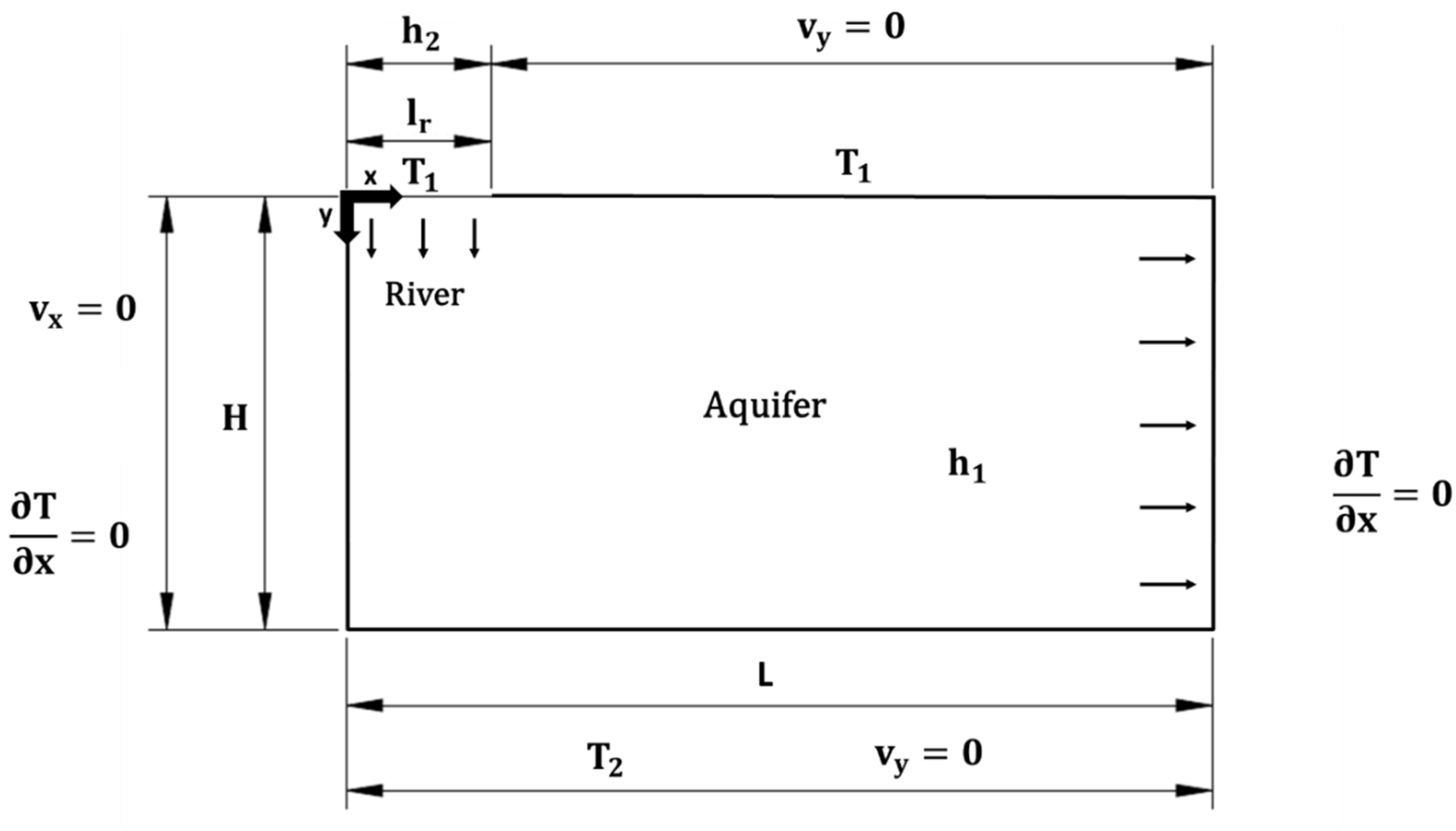
The physical scheme of the problem is shown in Figure 2. It depicts a saturated aquifer of anisotropic hydraulic conductivity that is impermeable at its bottom, with second-class homogeneous conditions or a Neumann condition (Equation (3)) and a water table coincident with the ground surface. The right border is the outflow region, while the left is impermeable (no flow) due to domain symmetry (half of the river); see Equation (3). Groundwater flow is imposed by constant potentials (first-class or Dirichlet conditions) at the river bottom (${\mathrm{h}}_2$) and potentials on the right border (${\mathrm{h}}_1$); see Equation (2). The thermal boundary conditions on the top and bed of the aquifer are temperatures ${\mathrm{T}}_1$ and ${\mathrm{T}}_2$, respectively, and Dirichlet conditions (constant values). On the left and right boundaries, there are adiabatic conditions (zero heat flux); see Equations (7)–(9).

The hydraulic problem, decoupled from the thermal problem, is characterized by a potential field $\mathrm{h}(\mathrm{x},\mathrm{y})$ resulting from the mechanical boundary conditions and the hydraulic conductivity. The flow lines go down below the streambed of the river and gradually curve until they become practically horizontal and equidistant (constant flow) beyond a certain extension. Regarding the temperature field $\mathrm{T}(\mathrm{x},\mathrm{y})$, there is a region in which the final temperature–depth profile develops. The extension in which the temperature–depth profile develops is called ${\mathrm{l}}_{\mathrm{T}}$. The mathematical model is gathered in the consequent set of equations:

The mechanical problem is presented as follows:

$${\mathrm{K}}_{\mathrm{x}}{\displaystyle \frac{{\partial }^2\mathrm{h}}{\partial {\mathrm{x}}^2}}+{\mathrm{K}}_{\mathrm{y}}{\displaystyle \frac{{\partial }^2\mathrm{h}}{\partial {\mathrm{y}}^2}}=0\left\{\begin{array}{c}{\displaystyle \frac{\partial {\mathrm{v}}_{\mathrm{x}}}{\partial \mathrm{x}}}+{\displaystyle \frac{\partial {\mathrm{v}}_{\mathrm{y}}}{\partial \mathrm{y}}}=0\\ {\mathrm{v}}_{\mathrm{x}}=-{\mathrm{K}}_{\mathrm{x}}{\displaystyle \frac{\partial \mathrm{h}}{\partial \mathrm{x}}} ; {\mathrm{v}}_{\mathrm{y}}={-\mathrm{K}}_{\mathrm{y}}{\displaystyle \frac{\partial \mathrm{h}}{\partial \mathrm{y}}}\end{array}\right.$$

(1)

$${\mathrm{h}}_{\left(0<\mathrm{x}<{\mathrm{l}}_{\mathrm{r}},\mathrm{y}=0\right)}={\mathrm{h}}_2$$

(2)

$${\left.{\displaystyle \frac{\partial \mathrm{h}}{\partial \mathrm{x}}}\right|}_{({\mathrm{l}}_{\mathrm{r}}\le \mathrm{x}\le \mathrm{L},0)}={\left.{\displaystyle \frac{\partial \mathrm{h}}{\partial \mathrm{y}}}\right|}_{(0,\mathrm{y})}={\left.{\displaystyle \frac{\partial \mathrm{h}}{\partial \mathrm{x}}}\right|}_{(\mathrm{x},\mathrm{H})}=0$$

(3)

$${\mathrm{h}}_{\left(\mathrm{L},\mathrm{y}\right)}={\mathrm{h}}_1$$

(4)

$$\overrightarrow{\mathrm{v}}=({\mathrm{v}}_{\mathrm{x}},{\mathrm{v}}_{\mathrm{y}})$$

(5)

The thermal problem is presented as follows:

$${\mathrm{k}}_{\mathrm{m},\mathrm{x}}{\displaystyle \frac{{\partial }^2\mathrm{T}}{\partial {\mathrm{x}}^2}}+{\mathrm{k}}_{\mathrm{m},\mathrm{y}}{\displaystyle \frac{{\partial }^2\mathrm{T}}{\partial {\mathrm{y}}^2}}-{\mathsf{\rho }}_{\mathrm{e},\mathrm{w}}{\mathrm{c}}_{\mathrm{e},\mathrm{w}}{\mathrm{v}}_{\mathrm{x}}{\displaystyle \frac{\partial \mathrm{T}}{\partial \mathrm{x}}}-{\mathsf{\rho }}_{\mathrm{e},\mathrm{w}}{\mathrm{c}}_{\mathrm{e},\mathrm{w}}{\mathrm{v}}_{\mathrm{y}}{\displaystyle \frac{\partial \mathrm{T}}{\partial \mathrm{y}}}=0$$

(6)

$${\mathrm{T}}_{(\mathrm{x}, \mathrm{y}=0)}={\mathrm{T}}_1$$

(7)

$${\mathrm{T}}_{(\mathrm{x}, \mathrm{y}=\mathrm{H})}={\mathrm{T}}_2$$

(8)

$${\left.{\displaystyle \frac{\partial \mathrm{T}}{\partial \mathrm{x}}}\right|}_{(\mathrm{x}=0, \mathrm{y})}=0$$

(9)

$${\left.{\displaystyle \frac{\partial \mathrm{T}}{\partial \mathrm{x}}}\right|}_{(\mathrm{x}=\mathrm{L}, \mathrm{y})}=0$$

(10)

Equation (1) is the result of combining the continuity equation for an incompressible fluid, ${\displaystyle \frac{\partial {\mathrm{v}}_{\mathrm{x}}}{\partial \mathrm{x}}}+{\displaystyle \frac{\partial {\mathrm{v}}_{\mathrm{y}}}{\partial \mathrm{y}}}=0$, with the Darcy equation for anisotropic media, ${\mathrm{v}}_{\mathrm{x}}={-\mathrm{K}}_{\mathrm{x}}{\displaystyle \frac{\partial \mathrm{h}}{\partial \mathrm{x}}};{\mathrm{v}}_{\mathrm{y}}=-{\mathrm{K}}_{\mathrm{y}}{\displaystyle \frac{\partial \mathrm{h}}{\partial \mathrm{y}}}$. Equation (6), which is the transport equation, includes both vertical and horizontal diffusivity terms. Finally, the initial temperature condition is obtained by solving the thermal problem in the absence of water flow. Although the same temperature was imposed on the entire upper boundary of the domain, the case in which the temperature of the river is different from the temperature of the ground on the surface is discussed later.

The numerical solution of the model is carried out using the network simulation method [28], which is a computational and accurate tool. An electrical network or circuit model with equations that are formally equivalent to those of the mathematical model is designed. The model is solved using a free circuit resolution program, Ngspice [29], which integrates the most powerful computing algorithms. The errors are reduced to negligible values (always <1%), the mesh sizes are of the order of 40 (vertical) versus 200 (horizontal), and the computation times are below 5 min for all the simulated cases.

3. Dimensionless Groups of the Problem and Verification

The dimensional characterization of the problem consists of the search for the dimensionless groups that govern both the hydraulic (decoupled) and thermal problems; the latter is coupled with the former. To infer the presence of these groups in anisotropic media with the greatest precision, discriminated dimensional analysis of the governing equations is applied. By assuming certain approximations in the derivative factors of the equations, the procedure leads to the smallest number of dimensionless groups and, therefore, to the most accurate solutions. In addition, the groups deduced through this technique can be physically interpreted in terms of the balances of the magnitudes that counteract each other throughout the domain. Therefore, their values are of a unified order of magnitude.

Firstly, the dependent and free variables are defined in a normalized and discriminated way, and duly justified references are introduced through physical reasoning. These variables are then substituted into the governing equation, reducing it to its dimensionless form. Finally, by approximating the derivative factors to unity following normalization, the resulting groups are the independent quotients between each pair of equation terms. Normalization, which forces the values of the dimensionless variables to range in the interval [0, 1], and discrimination, which assumes that quantities of vector character have different dimensions according to their spatial direction [30], leads to more precise results in scenarios with different values for K_x and K_y. The steps can be summarized as follows: (i) The dependent and independent variables are defined in a dimensionless way, and references are chosen so that the value of these variables is in the interval [0, 1]. Some of these references can be hidden or unknown magnitudes. (ii) Their substitution into the governing equation(s) obtains the mathematical model in a dimensionless form. (iii) The derivative factors are approximated to unity; this is made possible by the numerical range of the new variables. (iv) The groups are defined as the independent quotients between each pair of terms in the simplified equation.

As some of the unknowns of interest may have been introduced in the process, there might be some groups that contain such unknowns, which may result in two or more groups with the same unknown. However, through simple operations between groups, it is possible to set them in such a way that each of them contains a maximum of one unknown. Defined in this way, their physical meaning is in terms of balances.

Once the unknown has been obtained, the pi theorem is applied to define the dimensionless expressions of the unknowns as functions of the derived dimensionless groups without the unknowns that govern the solution and, eventually, as a function of the dimensionless positions and times. These dependencies are corroborated through numerical simulations of suitably chosen scenarios, and the dependencies themselves are shown by means of a universal set of curves after a high number of precise numerical simulations. The network simulation method [28] is used as a numerical tool; its efficiency and precision have been tested in numerous works [31,32,33].

3.1. The Mechanical Problem

Dimensionless variables are defined in the form

$$\mathrm{x}\mathrm{\prime }={\displaystyle \frac{\mathrm{x}}{\mathrm{L}}};\mathrm{y}\mathrm{\prime }={\displaystyle \frac{\mathrm{y}}{\mathrm{H}}}; \mathrm{h}\mathrm{\prime }={\displaystyle \frac{\mathrm{h}-{\mathrm{h}}_1}{{\mathrm{h}}_2-{\mathrm{h}}_1}}$$

(11)

These variables are replaced in Equation (1):

$${\mathrm{K}}_{\mathrm{x}}{\displaystyle \frac{{\partial }^2\mathrm{h}\mathrm{\prime }({\mathrm{h}}_2-{\mathrm{h}}_1)}{\partial {\mathrm{x}\mathrm{\prime }}^2{\mathrm{L}}^2}}+{\mathrm{K}}_{\mathrm{y}}{\displaystyle \frac{{\partial }^2\mathrm{h}\mathrm{\prime }({\mathrm{h}}_2-{\mathrm{h}}_1)}{\partial {\mathrm{y}\mathrm{\prime }}^2{\mathrm{H}}^2}}=0$$

(12)

Averaging or approximating the derivative factors within the whole scenario to unity, the resulting coefficients of the addends of the above equation are ${\displaystyle \frac{{\mathrm{K}}_{\mathrm{x}}}{{\mathrm{L}}^2}}$ and ${\displaystyle \frac{{\mathrm{K}}_{\mathrm{y}}}{{\mathrm{H}}^2}}$. From them, a single dimensionless group is deduced:

$${\mathrm{\pi }}_1={\displaystyle \frac{{\mathrm{K}}_{\mathrm{x}}}{{\mathrm{L}}^2}}{\displaystyle \frac{{\mathrm{H}}^2}{{\mathrm{K}}_{\mathrm{y}}}}$$

(13)

To this group, a discriminated group associated with the specific geometry of the problem must be added. It is generally denominated as the shape factor or aspect ratio, which defines the quotient between the horizontal extension of the river and that of the entire domain:

$${\mathrm{\pi }}_2={\displaystyle \frac{{\mathrm{l}}_{\mathrm{r}}}{\mathrm{L}}}$$

(14)

Thus, ${\mathrm{\pi }}_1$ and ${\mathrm{\pi }}_2$ necessarily control all the unknowns of the problem: dimensionless iso-potential (hydraulic) line patterns and dimensionless iso-streamline patterns. Moreover, such groups control the flow in its dimensionless form ${\displaystyle \frac{\mathrm{Q}}{({\mathrm{h}}_2-{\mathrm{h}}_1)\sqrt{{\mathrm{K}}_{\mathrm{x}}{\mathrm{K}}_{\mathrm{y}}}}}$ [34]. The pi theorem is applied:

$${\displaystyle \frac{\mathrm{Q}}{({\mathrm{h}}_2-{\mathrm{h}}_1)\sqrt{{\mathrm{K}}_{\mathrm{x}}{\mathrm{K}}_{\mathrm{y}}}}}={\mathrm{f}}_1\left({\displaystyle \frac{{\mathrm{K}}_{\mathrm{x}}}{{\mathrm{L}}^2}}{\displaystyle \frac{{\mathrm{H}}^2}{{\mathrm{K}}_{\mathrm{y}}}},{\displaystyle \frac{{\mathrm{l}}_{\mathrm{r}}}{\mathrm{L}}}\right)$$

(15)

The dimensionless potentials field depends on the relative positions $\mathrm{x}/\mathrm{L}$ and $\mathrm{y}/\mathrm{H}$:

$${\displaystyle \frac{\mathrm{h}-{\mathrm{h}}_1}{{\mathrm{h}}_2-{\mathrm{h}}_1}}={\mathrm{f}}_2\left({\displaystyle \frac{{\mathrm{K}}_{\mathrm{x}}}{{\mathrm{L}}^2}}{\displaystyle \frac{{\mathrm{H}}^2}{{\mathrm{K}}_{\mathrm{y}}}},{\displaystyle \frac{{\mathrm{l}}_{\mathrm{r}}}{\mathrm{L}}},{\displaystyle \frac{\mathrm{x}}{\mathrm{L}}},{\displaystyle \frac{\mathrm{y}}{\mathrm{H}}}\right)$$

(16)

It should be noted that discrimination, which is already applied in the very definition of the dimensionless variables (Equation (11)), leads to a more precise solution compared to that deduced from classical dimensionless considerations. From the latter, the group ${\displaystyle \frac{{\mathrm{K}}_{\mathrm{x}}}{{\mathrm{L}}^2}}{\displaystyle \frac{{\mathrm{H}}^2}{{\mathrm{K}}_{\mathrm{y}}}}$ is separated into two monomials, ${\displaystyle \frac{{\mathrm{K}}_{\mathrm{x}}}{{\mathrm{K}}_{\mathrm{y}}}}$ and ${\displaystyle \frac{\mathrm{H}}{\mathrm{L}}}$, which, as is to be verified, are not independent dimensionless groups.

For the values of ${\mathrm{\pi }}_1$ and ${\mathrm{\pi }}_2$, it should be noted that ${\displaystyle \frac{{\mathrm{l}}_{\mathrm{r}}}{\mathrm{L}}}$, which is not deduced from the governing equations but from the domain geometry, has a small value in general and has no physical meaning in terms of the balance of magnitudes, while ${\displaystyle \frac{{\mathrm{K}}_{\mathrm{x}}}{{\mathrm{L}}^2}}{\displaystyle \frac{{\mathrm{H}}^2}{{\mathrm{K}}_{\mathrm{y}}}}$ balances the horizontal and vertical velocity components. When the order of magnitude of this group is greater than unity (${\mathrm{K}}_{\mathrm{x}}$ >> ${\mathrm{K}}_{\mathrm{y}}$ or $\mathrm{H}$ >> $\mathrm{L}$, or both), the flow is confined to a region very close to the surface, and the pattern is independent of $\mathrm{H}$. If the value of this group is less than unity, the flow is distributed throughout the domain, creating a pattern clearly dependent on $\mathrm{H}$. As the boundary condition at the right of the domain implies a zero vertical velocity component (constant potential), very large domains would be similar to large regions where the vertical velocity component would be almost zero near the right edge.

To verify Equation (15), the numerical solution of the set of cases shown in

Table 1. Verification of expression (14).

Scenario	${\mathbf{K}}_{\mathbf{x}}$ (m·s−1)	${\mathbf{K}}_{\mathbf{y}}$ (m·s−1)	$\mathbf{H}$ (m)	${\mathbf{l}}_{\mathbf{r}}$ (m)	$\mathbf{L}$ (m)	${\mathbf{h}}_2-{\mathbf{h}}_1$ (m)	Q (m2 ·s−1)
1	5 × 10−5	1 × 10−5	10	10	100	0.1	479.9 × 10−9
2	1 × 10−4	2 × 10−5	10	10	100	0.05	479.9 × 10−9
3	1 × 10−4	2 × 10−5	20	20	200	0.1	959.8 × 10−9
4	5 × 10−5	1 × 10−5	20	20	200	0.2	959.8 × 10−9

is used. The illustrative scenarios (17 in total, introduced in Table 1,

Table 2. Parameter values of different scenarios.

Case	${\mathbf{k}}_{\mathbf{x}}$ (m·s−1)	${\mathbf{k}}_{\mathbf{y}}$ (m·s−1)	$\mathbf{H}$ (m)	$\mathbf{L}$ (m)	${\mathbf{l}}_{\mathbf{r}}$ (m)	$\frac{{\mathbf{k}}_{\mathbf{x}}{\mathbf{H}}^2}{{\mathbf{k}}_{\mathbf{y}}{\mathbf{L}}^2}$
5	2 × 10−4	2 × 10−5	10.00	100.00	10.00	0.10
6	2 × 10−4	8 × 10−5	40.00	200.00	20.00	0.10
7	10−4	10−5	10.00	100.00	10.00	0.10
8	10−4	10−5	22.36	100.00	10.00	0.50
9	10−4	10−5	15.82	50.00	5.00	1.00
10	10−4	10−5	35.35	50.00	5.00	5.00
11	10−4	10−5	25.00	25.00	2.50	10.00

and

Table 3. Verification of thermal length (${\mathrm{l}}_{\mathrm{T}}$) dependence.

Scenario	$\mathbf{H}$ (m)	${\mathbf{l}}_{\mathbf{r}}$ (m)	${\mathbf{K}}_{\mathbf{x}}$ (m·s−1)	${\mathbf{K}}_{\mathbf{y}}$ (m·s−1)	${\mathbf{h}}_2-{\mathbf{h}}_1$ (m)	${\mathbf{k}}_{\mathbf{m}}$ (cals−1 m−1 °C−1)	${\mathbf{\rho }}_{\mathbf{e,w}}{\mathbf{c}}_{\mathbf{e,w}}$ (calm−3 °C−1)	${\mathbf{l}}_{\mathbf{T}}$ (m)
12	40.0	5.0	1 × 10−5	1 × 10−5	2.0	1.0	1 × 106	86.50
13	20.0	2.5	1 × 10−5	1 × 10−5	2.0	1.0	1 × 106	43.25
14	20.0	2.5	2 × 10−5	2 × 10−5	2.0	2.0	1 × 106	43.25
15	40.0	5.0	1 × 10−5	1 × 10−5	4.0	2.0	1 × 106	86.50
16	120.0	15.0	4 × 10−5	4 × 10−5	4.0	8.0	1 × 106	259.50
17	40.0	5.0	1 × 10−5	1 × 10−5	2.0	2.0	2 × 106	86.50

) are simulated with arbitrary values of geometric and hydraulic properties, which are clearly different from each other. With these, even if a parameter’s value is changed from one case to another when the monomial does not change, the dimensionless result does not change either. This confirms that the dimensionless groups are correct; the relation between them, obtained using the strict formal protocol of the pi theorem and the type curves elaborated from these relations, leads to the expected solutions. For the scenarios in Table 1, the values of the monomials ${\mathrm{\pi }}_1$ and ${\mathrm{\pi }}_2$ are kept constant for all the scenarios, obtaining the same dimensionless flow rate ${\displaystyle \frac{\mathrm{Q}}{({\mathrm{h}}_2-{\mathrm{h}}_1)\sqrt{{\mathrm{K}}_{\mathrm{x}}{\mathrm{K}}_{\mathrm{y}}}}}$ = 0.215. The values of the lumped parameters are ${\displaystyle \frac{{\mathrm{K}}_{\mathrm{x}}}{{\mathrm{L}}^2}}{\displaystyle \frac{{\mathrm{H}}^2}{{\mathrm{K}}_{\mathrm{y}}}}$ = 5 and ${\displaystyle \frac{{\mathrm{l}}_{\mathrm{r}}}{\mathrm{L}}}$ = 0.1.

In scenarios 1 and 2, the values of ${\mathrm{K}}_{\mathrm{x}}$, ${\mathrm{K}}_{\mathrm{y}}$, and ${\mathrm{h}}_2-{\mathrm{h}}_1$ ($∆\mathrm{h}$) are modified to keep ${\displaystyle \frac{{\mathrm{K}}_{\mathrm{x}}{\mathrm{H}}^2}{{\mathrm{L}}^2{\mathrm{K}}_{\mathrm{y}}}}$ and ${\displaystyle \frac{{\mathrm{l}}_{\mathrm{r}}}{\mathrm{L}}}$ constant. It can be seen that the recharge flow $\mathrm{Q}$ and the dimensionless recharge flow $\left({\displaystyle \frac{\mathrm{Q}}{\left({\mathrm{h}}_2-{\mathrm{h}}_1\right)\sqrt{{\mathrm{K}}_{\mathrm{x}}{\mathrm{K}}_{\mathrm{y}}}}}\right)$ remain constant. In scenarios 3 and 4, the values of ${\mathrm{K}}_{\mathrm{x}}$, ${\mathrm{K}}_{\mathrm{y}}$ are modified, as is the geometry of the domain ($\mathrm{H}$, $\mathrm{L},$ and ${\mathrm{l}}_{\mathrm{r}}$), retaining the values of the groups ${\displaystyle \frac{{\mathrm{K}}_{\mathrm{x}}{\mathrm{H}}^2}{{\mathrm{L}}^2{\mathrm{K}}_{\mathrm{y}}}}$ and ${\displaystyle \frac{{\mathrm{l}}_{\mathrm{r}}}{\mathrm{L}}}$. As expected, the recharge flow doubles while the dimensionless discharge retains its value. The heat transport requires the separation of ${\displaystyle \frac{{\mathrm{K}}_{\mathrm{x}}}{{\mathrm{L}}^2}}{\displaystyle \frac{{\mathrm{H}}^2}{{\mathrm{K}}_{\mathrm{y}}}}$ into two independent groups since the thermal conductivity is isotropic. Consequently, the thermal problem depends on a high number of monomials. This creates additional complexity when it comes to defining the universal set of type curves.

Table 2 contains a set of cases (in which some of the physical and/or geometric parameters vary) that allow us to represent universal solutions associated with the values ${\mathrm{\pi }}_1$= 0.1, 0.5, 1, 5, and 10. For all cases, ${\mathrm{h}}_2-{\mathrm{h}}_1$= 1.00 m and ${\displaystyle \frac{{\mathrm{l}}_{\mathrm{r}}}{\mathrm{L}}}$ = 0.10.

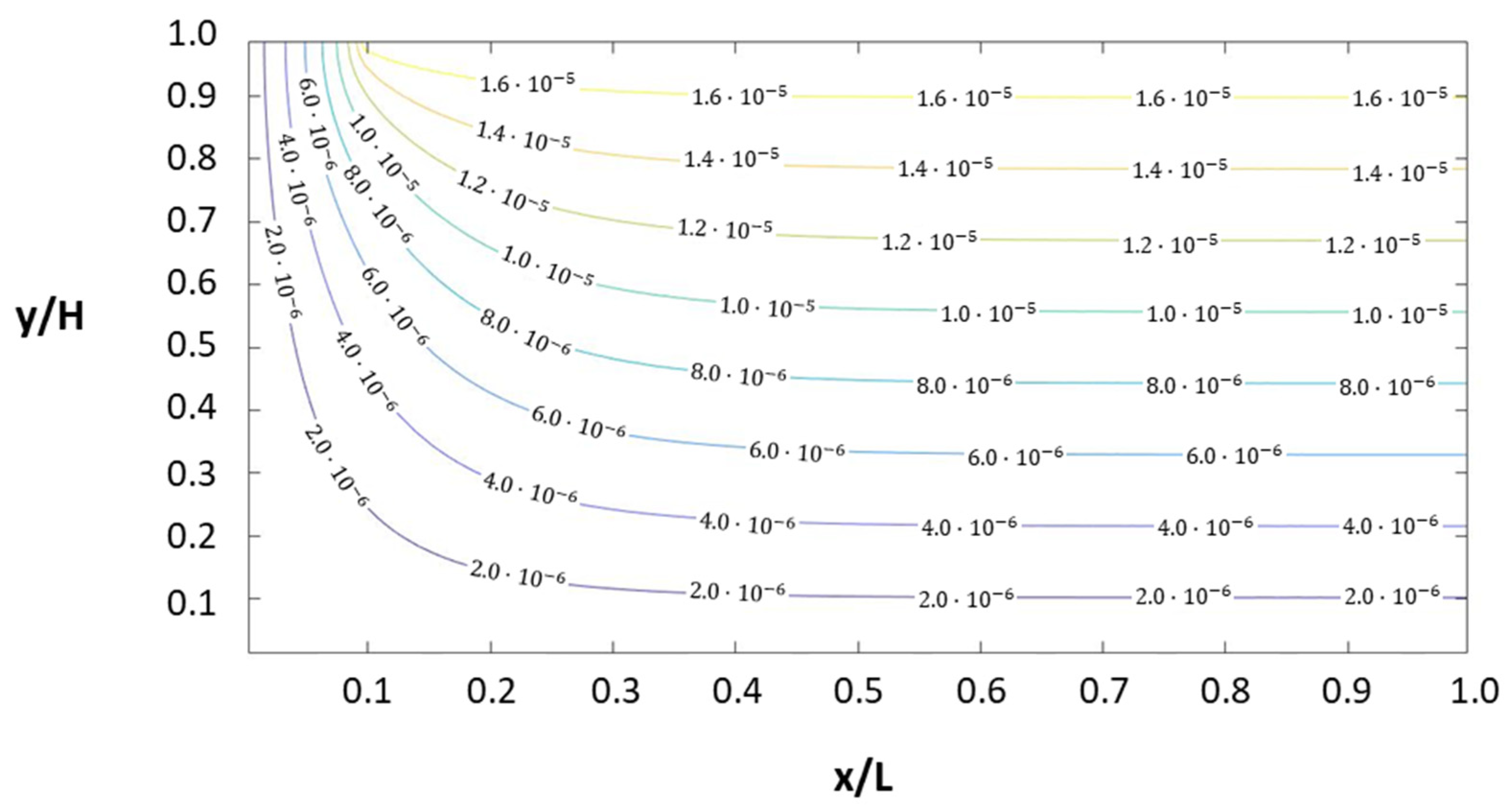
Figure 3 represents the pattern of flow lines for case 5. It shows groundwater velocity in each line, deduced from expression (15). This pattern, at first glance, separates two regions within the aquifer: the first, with velocity components ${\mathrm{v}}_{\mathrm{x}}$ and ${\mathrm{v}}_{\mathrm{y}}$ that are comparable with each other, and the second, where groundwater flow is markedly horizontal. Cases 6 and 7 have a similar pattern as they keep the same value of ${\mathrm{\pi }}_1$ and ${\mathrm{\pi }}_2$, but the flow is deduced from the previous one using the expression.

$${\displaystyle \frac{{\mathrm{Q}}_{\mathrm{C}\mathrm{a}\mathrm{s}\mathrm{e} 5}}{{\left\{({\mathrm{h}}_2-{\mathrm{h}}_1)\sqrt{{\mathrm{K}}_{\mathrm{x}}{\mathrm{K}}_{\mathrm{y}}}\right\}}_{\mathrm{C}\mathrm{a}\mathrm{s}\mathrm{e} 5}}}={\displaystyle \frac{{\mathrm{Q}}_{\mathrm{C}\mathrm{a}\mathrm{s}\mathrm{e} 6}}{{\left\{({\mathrm{h}}_2-{\mathrm{h}}_1)\sqrt{{\mathrm{K}}_{\mathrm{x}}{\mathrm{K}}_{\mathrm{y}}}\right\}}_{\mathrm{C}\mathrm{a}\mathrm{s}\mathrm{e} 6}}}={\displaystyle \frac{{\mathrm{Q}}_{\mathrm{C}\mathrm{a}\mathrm{s}\mathrm{e} 7}}{{\left\{({\mathrm{h}}_2-{\mathrm{h}}_1)\sqrt{{\mathrm{K}}_{\mathrm{x}}{\mathrm{K}}_{\mathrm{y}}}\right\}}_{\mathrm{C}\mathrm{a}\mathrm{s}\mathrm{e} 7}}}$$

(17)

3.2. The Thermal Problem

To obtain the dependencies in the thermal problem, it is necessary to define a region of thermal influence. This region is set using a thermal length (${\mathrm{l}}_{\mathrm{T}}$), which is defined as the longitude in which the thermal changes due to changes in water velocity are appreciable. For example, at a depth $\mathrm{y}=\mathrm{H}/2$, using the temperature interval defined as the difference between the temperature at the center of the river and that at the left edge of the domain, the value ${\mathrm{l}}_{\mathrm{T}}$ guarantees that 95% of the steady temperature is reached. It is important to note that the total length ($\mathrm{L}$), in which a constant h value is imposed, is far away from the river. By introducing $\mathrm{x}\mathrm{\prime }={\displaystyle \frac{\mathrm{x}}{{\mathrm{l}}_{\mathrm{T}}}}$ and $\mathrm{y}\mathrm{\prime }={\displaystyle \frac{\mathrm{y}}{\mathrm{H}}}$ (previously deduced) into governing Equation (6), deleting the derivative factors, and averaging, the resulting terms are ${\displaystyle \frac{{\mathrm{k}}_{\mathrm{m},\mathrm{x}}}{{{\mathrm{l}}_{\mathrm{T}}}^2}}$, ${\displaystyle \frac{{\mathrm{k}}_{\mathrm{m},\mathrm{y}}}{{\mathrm{H}}^2}}$, ${\displaystyle \frac{{\mathsf{\rho }}_{\mathrm{e},\mathrm{w}}{\mathrm{c}}_{\mathrm{e},\mathrm{w}}{\mathrm{K}}_{\mathrm{x}}({\mathrm{h}}_2-{\mathrm{h}}_1)}{{{\mathrm{l}}_{\mathrm{T}}}^2}}$, and ${\displaystyle \frac{{\mathsf{\rho }}_{\mathrm{e},\mathrm{w}}{\mathrm{c}}_{\mathrm{e},\mathrm{w}}{\mathrm{K}}_{\mathrm{y}}({\mathrm{h}}_2-{\mathrm{h}}_1)}{{\mathrm{H}}^2}}$. Assuming ${\mathrm{k}}_{\mathrm{m},\mathrm{x}}$ = ${\mathrm{k}}_{\mathrm{m},\mathrm{y}}={\mathrm{k}}_{\mathrm{m}}$, the independent quotients of these terms give rise to the following dimensionless groups:

$${\mathrm{\pi }}_3={\displaystyle \frac{{\mathrm{l}}_{\mathrm{T}}}{\mathrm{H}}}; {\mathrm{\pi }}_4={\displaystyle \frac{{\mathrm{K}}_{\mathrm{x}}}{{\mathrm{K}}_{\mathrm{y}}}}; {\mathrm{\pi }}_5={\displaystyle \frac{{\mathrm{k}}_{\mathrm{m}}}{{\mathsf{\rho }}_{\mathrm{e},\mathrm{w}}{\mathrm{c}}_{\mathrm{e},\mathrm{w}}{\mathrm{K}}_{\mathrm{y}}({\mathrm{h}}_2-{\mathrm{h}}_1)}}$$

(18)

A new monomial emerges due to the imposed boundary conditions ${\mathrm{\pi }}_6={\displaystyle \frac{{\mathrm{l}}_{\mathrm{r}}^2}{{\mathrm{H}}^2}}{\displaystyle \frac{{\mathrm{K}}_{\mathrm{x}}}{{\mathrm{K}}_{\mathrm{y}}}}$. As ${\mathrm{K}}_{\mathrm{x}}/{\mathrm{K}}_{\mathrm{y}}$ already exists as a dimensionless group, ${\mathrm{\pi }}_6$ can be simplified to ${\displaystyle \frac{{\mathrm{l}}_{\mathrm{r}}}{\mathrm{H}}}$. The pi theorem is applied:

$${\displaystyle \frac{{\mathrm{l}}_{\mathrm{T}}}{\mathrm{H}}}={\mathrm{Y}}_3\left({\mathrm{\pi }}_4, {\mathrm{\pi }}_5, {\mathrm{\pi }}_6\right)={\mathrm{f}}_3\left({\displaystyle \frac{{\mathrm{K}}_{\mathrm{x}}}{{\mathrm{K}}_{\mathrm{y}}}}, {\displaystyle \frac{{\mathrm{k}}_{\mathrm{m}}}{{\mathsf{\rho }}_{\mathrm{e},\mathrm{w}}{\mathrm{c}}_{\mathrm{e},\mathrm{w}}{\mathrm{K}}_{\mathrm{y}}({\mathrm{h}}_2-{\mathrm{h}}_1)}},{\displaystyle \frac{{\mathrm{l}}_{\mathrm{r}}}{\mathrm{H}}}\right)$$

(19)

Table 3 shows seven cases selected to verify solution (18). Compared to case 12, in case 13 the total depth of the aquifer, the length of the river, and the thermal length are multiplied by 0.5, keeping ${\mathrm{\pi }}_3$ constant. In case 14, the vertical and horizontal hydraulic conductivity and thermal conductivity are doubled, while ${\mathrm{l}}_{\mathrm{r}}$ and $\mathrm{H}$ are halved to obtain the same thermal length (${\mathrm{l}}_{\mathrm{T}}$) as that in case 13, as expected. In case 15, the thermal conductivity and ∆h are duplicated, keeping ${\mathrm{\pi }}_5$ constant and, as expected, obtaining the same value of ${\mathrm{l}}_{\mathrm{T}}$ as that in case 12.

In case 16, the hydraulic conductivities are quadrupled, the length of the river and the total depth of the aquifer are tripled, the value of $∆\mathrm{h}$ is doubled, and the thermal conductivity of the water–soil matrix is multiplied by eight. As expected, the thermal characteristic length is multiplied by three because the aquifer depth tripled and the monomials ${\mathrm{\pi }}_4$, ${\mathrm{\pi }}_5$, and ${\mathrm{\pi }}_6$ retained the same values. Finally, in case 17, both ${\mathrm{k}}_{\mathrm{m}}$ and ${\mathsf{\rho }}_{\mathrm{e},\mathrm{w}}{\mathrm{c}}_{\mathrm{e},\mathrm{w}}$ are duplicated, obtaining the same ${\mathrm{l}}_{\mathrm{T}}$ as that in case 12. For all the cases (scenarios 12 to 17), ${\mathrm{\pi }}_3$= 2.163, ${\mathrm{\pi }}_4$= 1.0, ${\mathrm{\pi }}_5$= 0.05, and ${\mathrm{\pi }}_6$= 0.125.

Within the thermal characteristic length (${\mathrm{l}}_{\mathrm{T}}$), the dimensionless temperature profiles are universal, which means the following:

$${\displaystyle \frac{\mathrm{T}-{\mathrm{T}}_1}{{\mathrm{T}}_2-{\mathrm{T}}_1}}={\mathrm{f}}_4\left({\displaystyle \frac{\mathrm{x}}{{\mathrm{l}}_{\mathrm{T}}}},{\displaystyle \frac{\mathrm{y}}{\mathrm{H}}}\right)$$

(20)

For general scenarios in which it is not known whether the thermal characteristic length is greater than the total length of the domain (distance between ${\mathrm{h}}_2$ and ${\mathrm{h}}_1$) or it is known that the total length of the domain is equal to or less than the thermal one, $\mathrm{x}\mathrm{\prime }={\displaystyle \frac{\mathrm{x}}{\mathrm{L}}}$ and, therefore, the dimensionless groups are as follows:

$${\mathrm{\pi }}_7={\displaystyle \frac{\mathrm{L}}{\mathrm{H}}}; {\mathrm{\pi }}_4={\displaystyle \frac{{\mathrm{K}}_{\mathrm{x}}}{{\mathrm{K}}_{\mathrm{y}}}}; {\mathrm{\pi }}_5={\displaystyle \frac{{\mathrm{k}}_{\mathrm{m}}}{{\mathsf{\rho }}_{\mathrm{e},\mathrm{w}}{\mathrm{c}}_{\mathrm{e},\mathrm{w}}{\mathrm{K}}_{\mathrm{y}}({\mathrm{h}}_2-{\mathrm{h}}_1)}}; {\mathrm{\pi }}_6={\displaystyle \frac{{\mathrm{l}}_{\mathrm{r}}}{\mathrm{L}}}$$

(21)

The corrected thermal diffusivity (${\mathsf{\alpha }}_{\mathrm{c}}$) is defined as the ratio of the thermal conductivity of the water–soil matrix (${\mathrm{k}}_{\mathrm{m}}$) to the specific heat of the water (${\mathsf{\rho }}_{\mathrm{e},\mathrm{w}}{\mathrm{c}}_{\mathrm{e},\mathrm{w}}$). Within the total length and depth of the domain, the dimensionless temperature is

$${\displaystyle \frac{\mathrm{T}-{\mathrm{T}}_1}{{\mathrm{T}}_2-{\mathrm{T}}_1}}={\mathrm{f}}_5\left({\displaystyle \frac{{\mathrm{K}}_{\mathrm{x}}}{{\mathrm{K}}_{\mathrm{y}}}}, {\displaystyle \frac{{\mathsf{\alpha }}_{\mathrm{c}}}{{\mathrm{K}}_{\mathrm{y}}({\mathrm{h}}_2-{\mathrm{h}}_1)}}, {\displaystyle \frac{\mathrm{L}}{\mathrm{H}}},{\displaystyle \frac{{\mathrm{l}}_{\mathrm{r}}}{\mathrm{L}}}, {\displaystyle \frac{\mathrm{x}}{\mathrm{L}}}, {\displaystyle \frac{\mathrm{y}}{\mathrm{H}}}\right)$$

(22)

4. Type Curves and Universal Dimensionless Temperature Surfaces

Figure 4 shows the set of curves for the dimensionless flow. When the monomial ${\mathrm{\pi }}_1$ is less than unity, it can be observed that this magnitude is not very sensitive to ${\mathrm{\pi }}_2$. However, when ${\mathrm{\pi }}_1$ > 1, the dimensionless flow depends appreciably on ${\mathrm{\pi }}_2$. The real flow Q (not dimensionless) does change appreciably. That is because it depends on $({\mathrm{h}}_2-{\mathrm{h}}_1)\sqrt{{\mathrm{k}}_{\mathrm{x}}{\mathrm{k}}_{\mathrm{y}}}$, whose value changes from one case to another (Equation (15)).

Figure 5 shows the type curves of dimensionless potential at $\mathrm{x}={\mathrm{l}}_{\mathrm{r}}$, with ${\displaystyle \frac{{\mathrm{l}}_{\mathrm{r}}}{\mathrm{L}}}=0.1$, and values of ${\displaystyle \frac{{\mathrm{K}}_{\mathrm{x}}}{{\mathrm{L}}^2}}{\displaystyle \frac{{\mathrm{H}}^2}{{\mathrm{K}}_{\mathrm{y}}}}$ = 0.1, 0.5, 1, 5, and 10. These universal type curves become more curved and reach small dimensionless values in scenarios in which the horizontal hydraulic conductivity and/or the horizontal extension of the aquifer are large compared to the vertical conductivity and/or the depth $\mathrm{H}$.

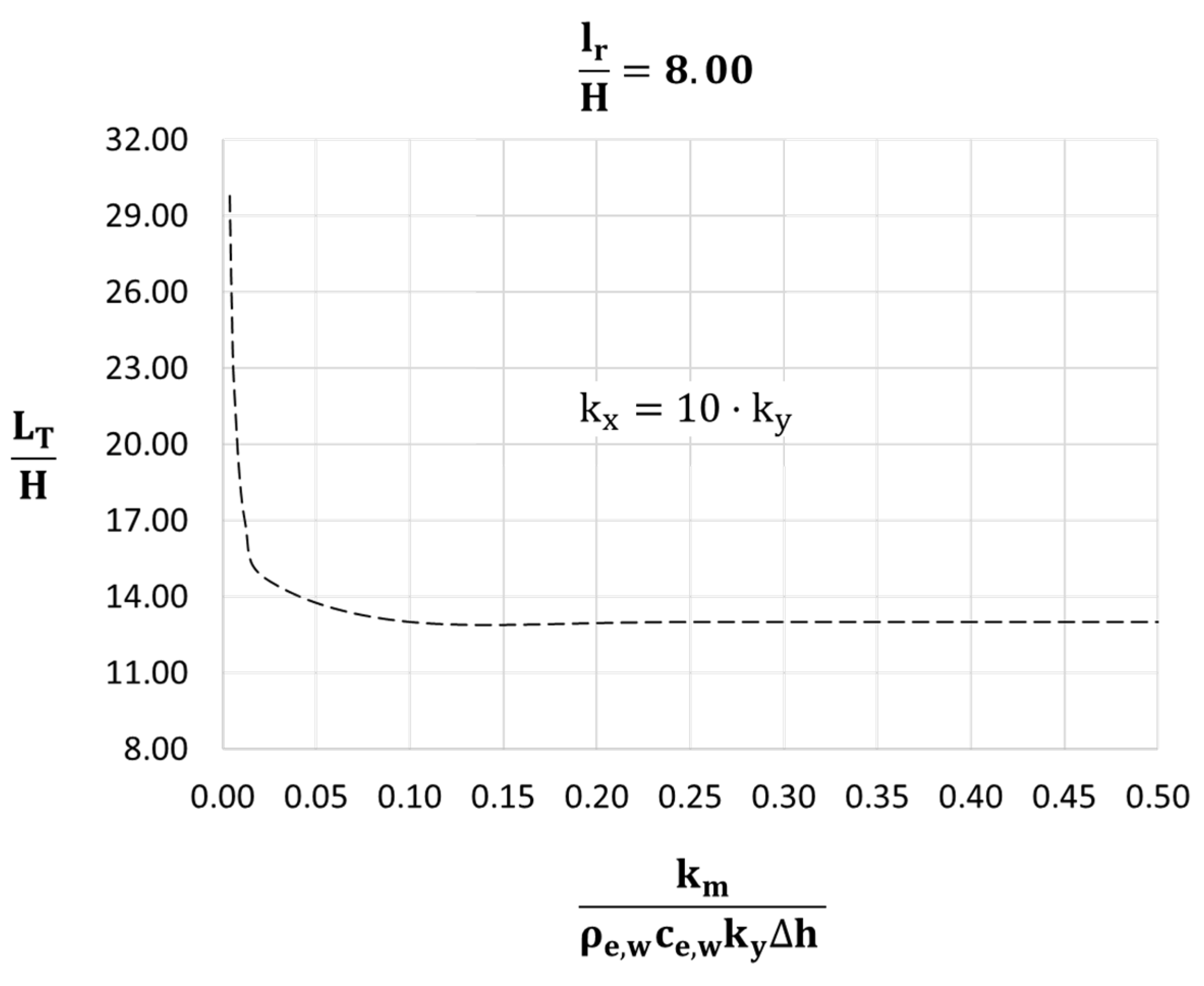
Figure 6 depicts Equation (19) in three different abacuses: the abacus parameter, the monomial ${\displaystyle \frac{{\mathrm{l}}_{\mathrm{r}}}{\mathrm{H}}}$, and the type curve parameter ${\displaystyle \frac{{\mathrm{K}}_{\mathrm{x}}}{{\mathrm{K}}_{\mathrm{y}}}}$. In the three sets of type curves, it can be seen that, for the values of ${\displaystyle \frac{{\mathrm{k}}_{\mathrm{m}}}{{\mathsf{\rho }}_{\mathrm{e},\mathrm{w}}{\mathrm{c}}_{\mathrm{e},\mathrm{w}}{\mathrm{K}}_{\mathrm{y}}\left({\mathrm{h}}_2-{\mathrm{h}}_1\right)}}$ under 0.2, ${\displaystyle \frac{{\mathrm{l}}_{\mathrm{T}}}{\mathrm{H}}}$ is strongly dependent on this monomial, especially for ${\displaystyle \frac{{\mathrm{K}}_{\mathrm{x}}}{{\mathrm{K}}_{\mathrm{y}}}}$ = 5 and ${\displaystyle \frac{{\mathrm{K}}_{\mathrm{x}}}{{\mathrm{K}}_{\mathrm{y}}}}$= 10. From this value, ${\displaystyle \frac{{\mathrm{l}}_{\mathrm{T}}}{\mathrm{H}}}$ remains constant. 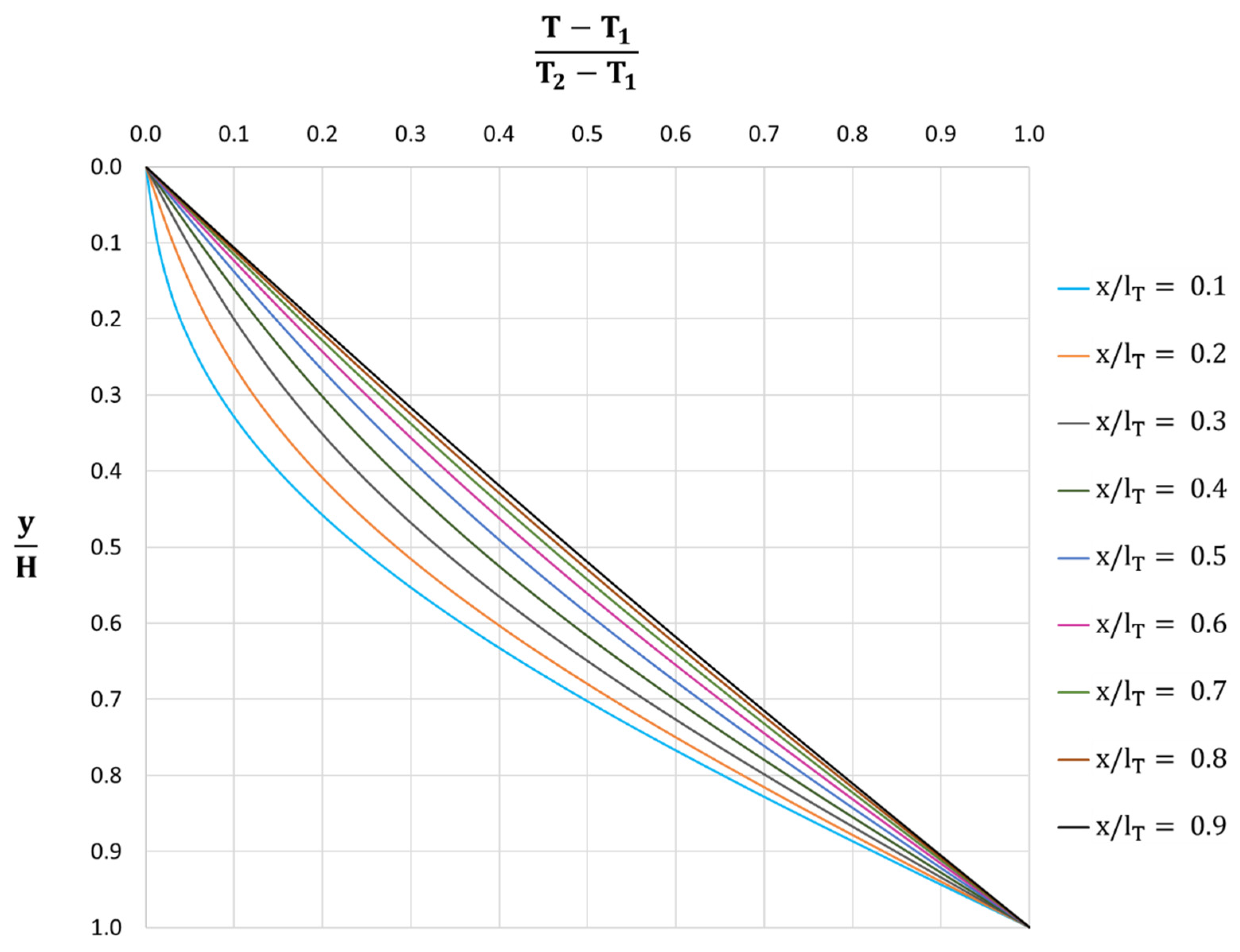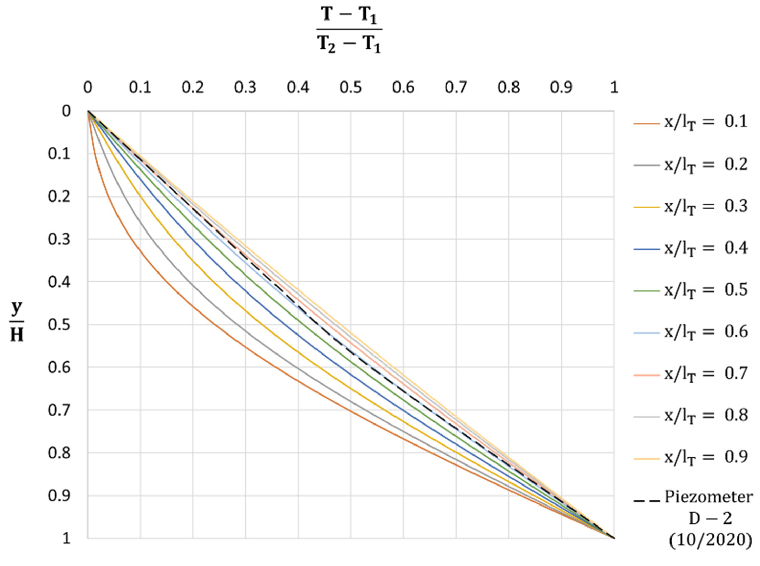Figure 7 represents the universal temperature profiles within the region defined by the thermal characteristic length (Equation (20)), for $\mathrm{x}/{\mathrm{l}}_{\mathrm{T}}$ values from 0.1 to 0.9. By recording the vertical temperature variations within the region bounded by ${\mathrm{l}}_{\mathrm{T}}$ and making use of the type curves in Figure 7, the value of ${\mathrm{l}}_{\mathrm{T}}$ can be estimated. By entering this thermal length in Figure 6, and knowing the hydraulic and geometric parameters of the problem, an estimate of the thermal conductivity of the soil–water matrix can be determined.

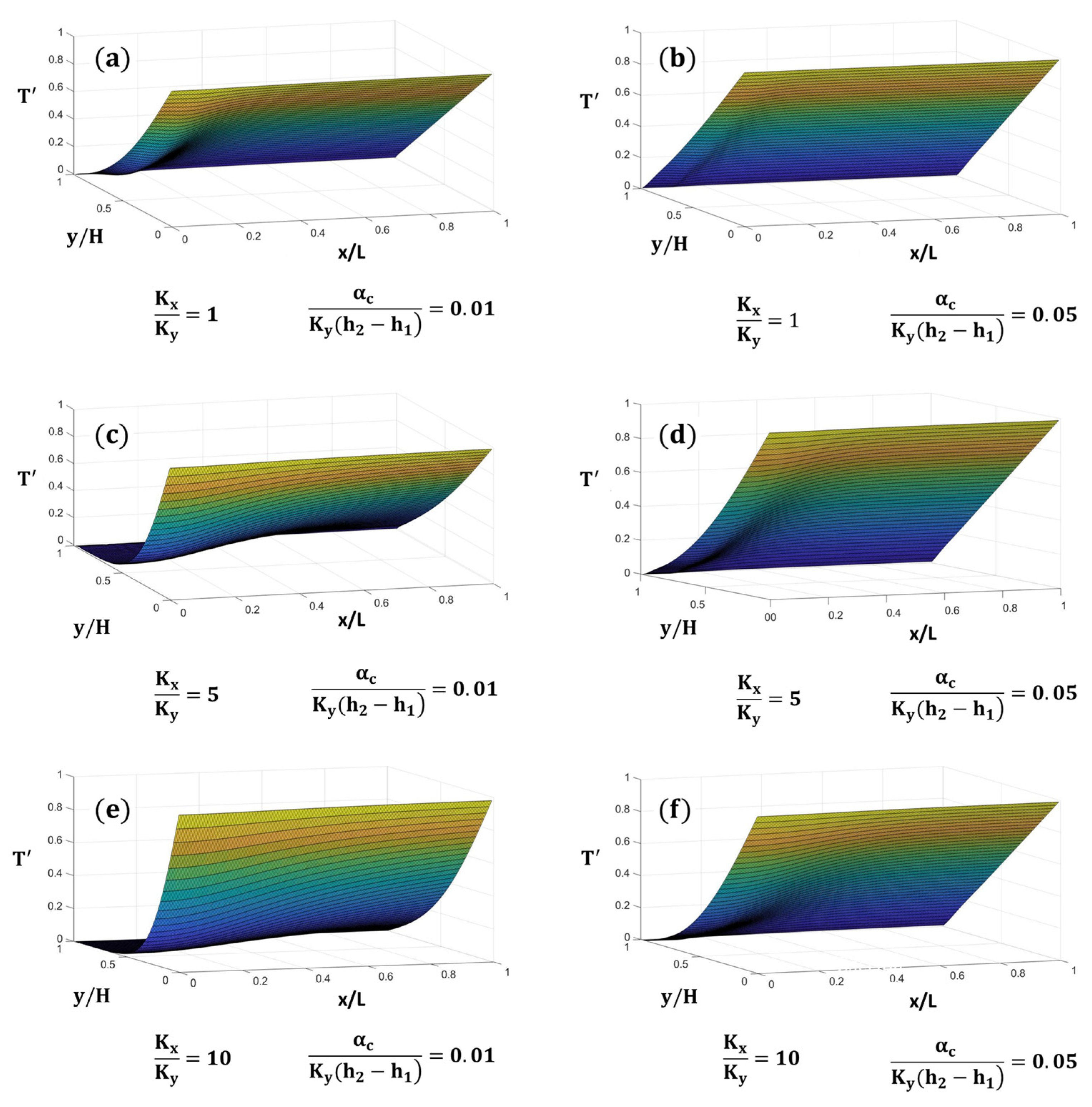
Finally, a set of universal surfaces for Equation (22) is shown in Figure 8. The representation of these surfaces is merely illustrative due to the large number of surfaces that would have been necessary to use them in practice. The elaboration of an extended compendium containing type curves raised from the new dimensionless group is left for further extended studies.

Figure 8 shows the universal surfaces. The parameters of each universal sheet (surface) are the quotient between the hydraulic conductivities ${\displaystyle \frac{{\mathrm{K}}_{\mathrm{x}}}{{\mathrm{K}}_{\mathrm{y}}}}$ and the dimensionless group ${\displaystyle \frac{{\mathsf{\alpha }}_{\mathrm{c}}}{{\mathrm{K}}_{\mathrm{y}}({\mathrm{h}}_2-{\mathrm{h}}_1)}}$. Each set of surfaces represents the same value for the shape factor ${\displaystyle \frac{{\mathrm{l}}_{\mathrm{r}}}{\mathrm{L}}}$.

5. Application to Case Study and Discussion

To verify the reliability of the solutions provided and their versatility, we applied the type curves to two real case studies: the discharge of the Guadalfeo River to the Motril-Salobreña aquifer and the artificial recharge of the Agua Amarga coastal aquifer in southern Spain. These hydrogeological systems have many uncertainties related to their geological features (heterogeneity, anisotropy, etc.); these uncertainties lead to some constraints and shortcomings in the analytical solutions [35]. Consequently, some assumptions and hypotheses had to be made regarding geometry and the mechanical or thermal properties. These assumptions are decisive in the verification of the accuracy of the validation.

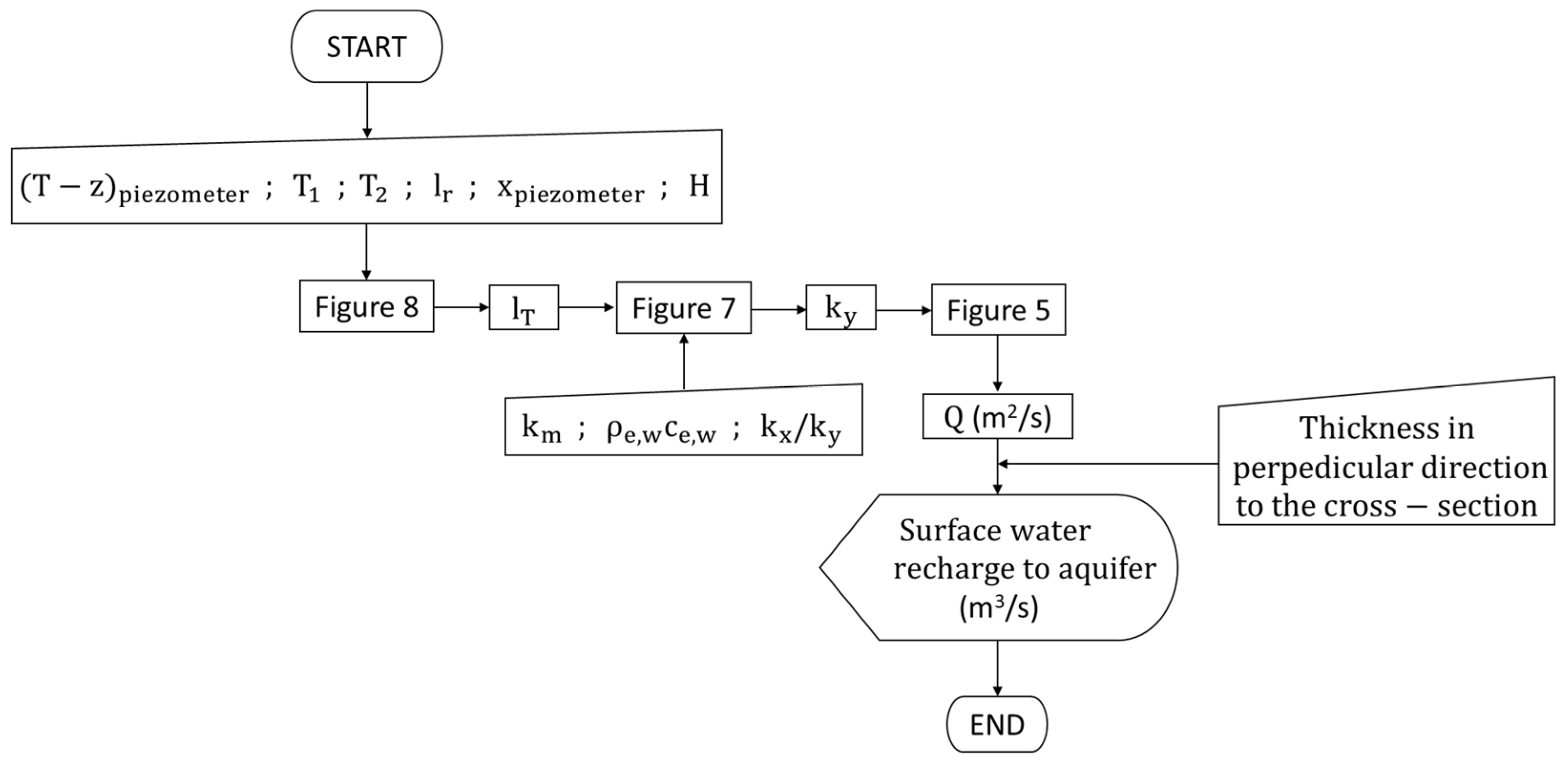
The procedure applied is outlined in Figure 9. In the case that there is a reliable value for both the hydraulic conductivity and its anisotropy, the value of the thermal conductivity of the saturated porous media can be obtained from Figure 6. If only the type of material is known and only a range of thermal conductivities and hydraulic conductivities is available, it is preferable to use thermal conductivity as input data since its range of variation is much smaller [8].

5.1. The Artificial Recharge Program in Agua Amarga

The Agua Amarga coastal aquifer has been subjected to anthropogenic intervention during the last century [36]. The artificial recharge of the aquifer over the protected salt marsh surface has been carried out regularly since 2008. This measure compensates for the negative effect on piezometry caused by groundwater abstraction from the pumping wells of the Alicante desalination plants. The measure has proven to be environmentally sustainable and has provided alternatives for salt marsh enhancement.

The verification of the type curves is applied to a 2D cross-section in the direction of the general flow and includes the piezometer P-8 located at the border of the flooded ponds (the recharge area) and the piezometer D-2 (Figure 10). The depression cone is located to the north, where 26 pumping wells are arranged parallel to the coastline.

In this case study, the recharge volume over the salt marsh (${\mathrm{l}}_{\mathrm{r}}$ = 350 m) was compared to that estimated from the temperature–depth profile in D-2, using a piezometer in the flow direction that was close enough to the marshes (390 m from the right border of the marshes) to ensure that the characteristic thermal length was larger. A period of constant recharge was selected (the year 2020), and a month in which the temperature–depth profile and the flooded ponds were known was chosen (October 2020). The flooded marshes had a width of approximately 100 m. The distance between the left boundary of the cross-section and the piezometer D-2 was 740 m. From the dimensionless temperature in Figure 11 and the universal set of curves in Figure 7, x/l_T = 0.60 was obtained; therefore, a length of l_T = 1233 m was obtained. This value was taken as “L” since it can be stated that, from this length, the groundwater flow is horizontal and, consequently, the thermal profiles are not affected by the recharge flow from the marshes. By using the universal curve (Figure 12, which had to be designed for this scenario due to the large value of the ${\displaystyle \frac{l_r}{H}}$ ratio, for the case when ${\mathrm{l}}_{\mathrm{r}}/\mathrm{H}$ = 8 (for H = 44 m), a value of $\left({\mathrm{k}}_{\mathrm{m}}\right)/({\mathsf{\rho }}_{\mathrm{e},\mathrm{w}}{\mathrm{c}}_{\mathrm{e},\mathrm{w}}·{\mathrm{k}}_{\mathrm{y}}·\mathrm{\Delta }\mathrm{h})$ = 0.0035 was obtained. Considering ${\mathrm{k}}_{\mathrm{m}}$ = 2.7 cal/(s·m·°C), ${\mathsf{\rho }}_{\mathrm{e},\mathrm{w}}{\mathrm{c}}_{\mathrm{e},\mathrm{w}}$ = 10⁶ cal/(m³·°C), and $\mathrm{\Delta }\mathrm{h}$ = 6.17 m (since the gradient equals 0.005), a vertical hydraulic conductivity ${\mathrm{k}}_{\mathrm{y}}$ = 10.8 m/d was obtained. Thus, the horizontal hydraulic conductivity was ${\mathrm{k}}_{\mathrm{x}}$ = 108 m/d.

Figure 4 can now be used to estimate the dimensionless flow rate ${\displaystyle \frac{\mathrm{Q}}{\left({\mathrm{h}}_2-{\mathrm{h}}_1\right)\sqrt{{\mathrm{K}}_{\mathrm{x}}{\mathrm{K}}_{\mathrm{y}}}}}$ = 0.151, giving a value of $\mathrm{Q}$ = 32.82 m²/d in the cross-section. Assuming 100 m of transversal extension (the pond stretch), the recharge flow from the irrigation marshes to the aquifer that reaches the piezometer D-2 is 3282 m³/d. In this month, the artificial recharge was 4167 m³/d, which was 80% of the estimated recharge.

5.2. The Guadalfeo River and Motril-Salobreña Aquifer Interaction

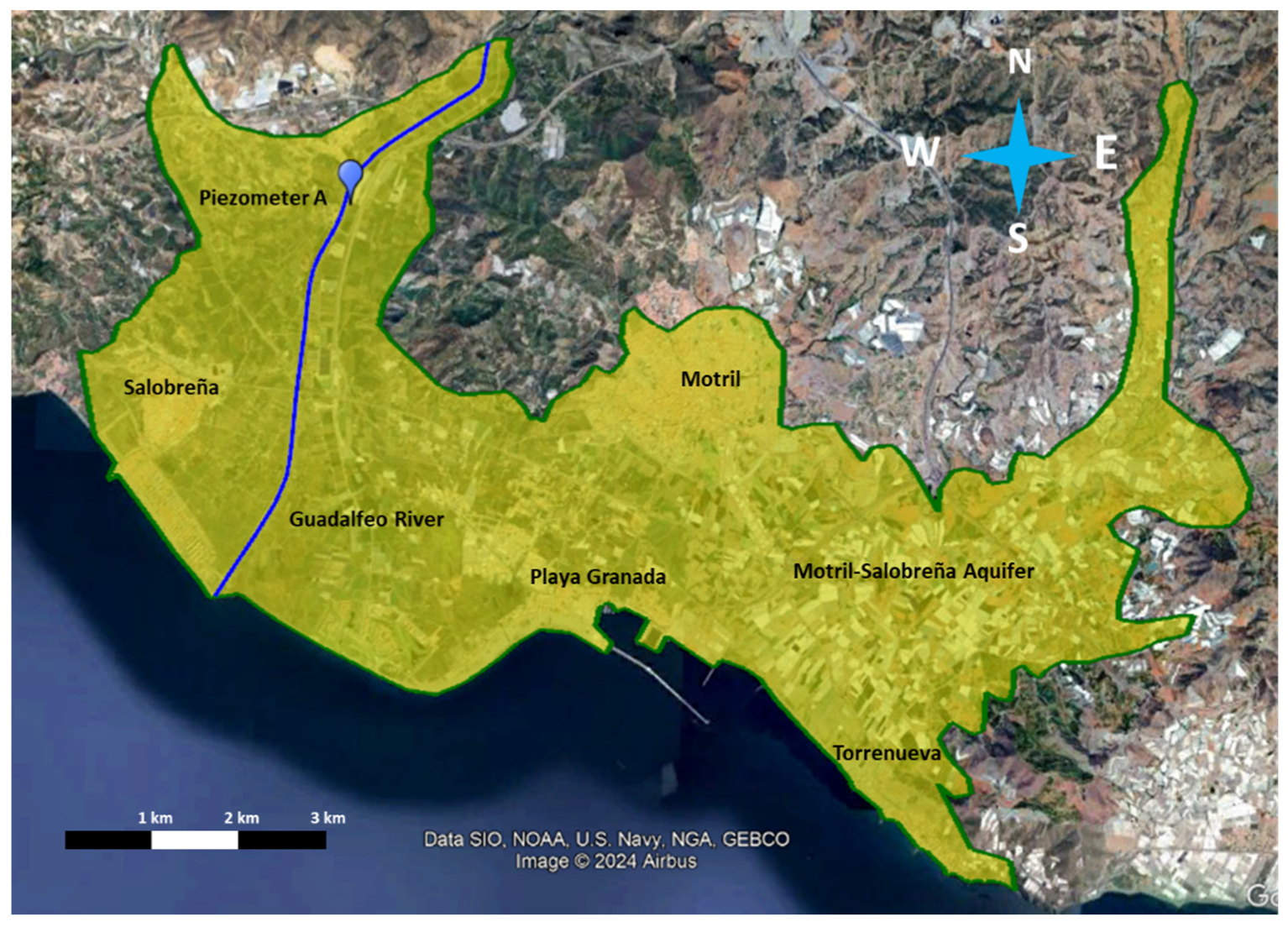
The Motril-Salobreña coastal aquifer is in the province of Granada (Southern Spain) (Figure 13). One of its main water inflows is the recharge from the Guadalfeo River, and this volume of water is very important to maintain the high quality of groundwater in the aquifer [18]. The aquifer is formed by sediments deposited by the Guadalfeo River and other ephemeral streams. The associated hydraulic conductivities vary from normal values for clays and silts to clean gravels. The depth of the aquifer is also highly variable, varying between 30 and 50 m in the northern zone (alluvial sedimentary medium) and reaching more than 250 m in the areas near the coast (deltaic sedimentary medium).

To estimate the recharge flow of the Guadalfeo River to the Motril-Salobreña aquifer, we used a temperature profile recorded with a piezometer in April 2002; it was located close to the river (70 m from its center) so that we could be sure that the borehole was within the thermal characteristic length. The profile was dimensioned in order to use the universal abacus in Figure 7 (see Figure 14). The half-width of the river is 15 m in this area.

Entering Figure 7 (see Figure 14) gives a value of $\mathrm{x}/{\mathrm{l}}_{\mathrm{T}}$ = 0.30 and, therefore, ${\mathrm{l}}_{\mathrm{T}}$ = 233.3 m. This value is taken as “L” since, from this length, the groundwater flow is horizontal, and the thermal profiles would not be affected by the recharge. By entering ${\mathrm{l}}_{\mathrm{r}}$ = 15 m and $\mathrm{H}$ = 14.5 m into Figure 6, a value of $\left({\mathrm{k}}_{\mathrm{m}}\right)/({\mathsf{\rho }}_{\mathrm{e},\mathrm{w}}{\mathrm{c}}_{\mathrm{e},\mathrm{w}}·{\mathrm{k}}_{\mathrm{y}}·\mathrm{\Delta }\mathrm{h})$ = 0.0075 is obtained. Considering ${\mathrm{k}}_{\mathrm{m}}$ = 0.694 cal/(s·m·°C) [37], ${\mathsf{\rho }}_{\mathrm{e},\mathrm{w}}{\mathrm{c}}_{\mathrm{e},\mathrm{w}}$ = 10⁶ cal/(m³·°C) and $\mathrm{\Delta }\mathrm{h}$ = 19.13 m, a vertical hydraulic conductivity ${\mathrm{k}}_{\mathrm{y}}$ = 4.84 × 10⁻⁶ m/s is obtained. As the anisotropy is ${\mathrm{k}}_{\mathrm{x}}/{\mathrm{k}}_{\mathrm{y}}$ = 10, the horizontal hydraulic conductivity is ${\mathrm{k}}_{\mathrm{x}}$ = 4.84 × 10⁻⁵ m/s.

The universal curve ${\mathrm{l}}_{\mathrm{r}}/\mathrm{L}$ = 0.1 in Figure 4 is used to estimate the recharge flow rate, as its dimensionless value equals 0.194. The recharge flow rate in this aquifer section (to be multiplied by 2 due to symmetry) is 5.72 × 10⁻⁵ m²/s. As the length perpendicular to the section in which the value of the recharge is known is 1100 m, the total river recharge to the aquifer in this zone is 0.126 m³/s. The estimate made by Duque et al. [18] was around 0.145 m³/s; thus, the difference between the two is less than 15%, which is a more than acceptable result.

5.3. Result Discussion

In the case of the Agua Amarga coastal aquifer, the effect of regional flow from the continent on the temperature–depth profile was disregarded since possible sources of aquifer recharge were high enough to generate steady temperature–depth profiles near the coastline. The horizontal flow of this aquifer comes primarily from the Campo de Elche region, an agricultural area in the province of Alicante located approximately 15 km from the marshes The effect of the seawater intrusion wedge was also neglected because the depression cone directs seawater flow to the aquifer [14,36]. The uncertainties were related to the aquifer thickness (ranging from 10 to 60 m inside the aquifer limits) and the hydraulic conductivity parameters, which were estimated using a pumping test between 16 and 150 m/d. Furthermore, the aquifer was assumed to be confined, although the heterogeneity of the Quaternary sediments covering the ground surface made the underlying Tyrrhenian aquifer behave as a free aquifer next to the coastline. It is also important to note that no evaporation from the ponds, which is estimated to be 850 mm/year, was considered. The possible loss of water through Quaternary faults, percolating to the geological formation under the studied Tyrrhenian aquifer, was also not considered. These factors might justify the lower calculated values. Although the real and calculated values were of the same order of magnitude, all these circumstances should have influenced the differences, and a 20% error in the findings would be reasonable. In the previous studies, Alhama [14] discussed the influence of artificial recharge on the piezometer D-2 in the 2008–2010 period, supporting the results on the relative shape of the temperature–depth profiles of six piezometers and on the outcomes of a fluid flow and solute transport numerical model made using Moldflow [36]. The results presented here verify his conclusions and match the recharge volumes used.

In this scenario, the thermal parameters are well known and there is a very wide range of possible values for hydraulic conductivity. Therefore, the thermal conductivity of the saturated porous media was taken from the input data to estimate the value of the vertical hydraulic conductivity and, assuming an anisotropy value of 10, the value of the horizontal hydraulic conductivity. The estimated value of the vertical hydraulic conductivity was ${\mathrm{k}}_{\mathrm{y}}$ = 10.8 m/d, while that of ${\mathrm{k}}_{\mathrm{x}}$ = 108 m/d. Both values were within the initially known range [16–150 m/d]; therefore, the results were as expected. The flow obtained in Figure 4 is the flow that directly reaches borehole D-2 from the artificial recharge and, since there is no symmetry (the water goes directly from the marshes to borehole D-2), it is not necessary to multiply the recharge value by two (as would occur in the case of a classic scenario of river–aquifer interaction).

As for the Guadalfeo River–Motril-Salobreña aquifer interaction, one of the major difficulties was, on the one hand, the value given to ${\mathrm{l}}_{\mathrm{r}}$, since there were no aerial photographs of the area in the period in which the temperatures were recorded in piezometer A. It was decided to take an average value that was consistent with the different piezometry values between the river and piezometer A. On the other hand, the exact value of $\mathrm{H}$ to be considered was not known. In this case, as this value was used to solve the thermal problem, it was easy to accept the depth from which the temperature no longer varied due to thermal changes caused by river recharge as a value. In this case, as in the previous application of artificial irrigation, the thermal conductivity in the porous media was better known than the hydraulic conductivity. Therefore, the hydraulic conductivity was also estimated as a function of the thermal parameters. The estimate of river recharge to the aquifer made by Duque et al. [18] was around 0.145 m³/s; thus, the difference between the estimates was less than 15%, which was a more than acceptable result considering the associated uncertainties.

The type curves presented here were applied to general cases of SW–GW interactions (rivers, lakes) and were not limited to the specific boundary conditions defined in other studies, such as imposed horizontal flow [38] or fine confined layers with horizontal flow [16]. The quantitative contribution of type curves goes further than the qualitative descriptions reported in previous works, in which the estimation of infiltration zones and the relative vertical–horizontal components in groundwater or the relative vertical flows in small rivers or infiltration areas were reported [15,17,36]. The methodology (non-dimensionalization) can be generally applied since the analytical solutions are not based on experimental correlations.

However, the case study to be applied must meet some geometrical constraints: (i) the distance between the recharge region and the piezometer where the temperatures are recorded must be short enough to guarantee the absence of a single horizontal flow; (ii) the total length of the domain must be large enough to allow a region of temperature profile development from which the groundwater velocity can be considered horizontal.

Additionally, the aquifer is assumed to be saturated; thus, the results can only be applied to a confined aquifer or an unconfined aquifer with a low gradient and full saturation. Finally, if there is a boundary condition downstream of the recharge area (on the right side of the cross-section), the estimated value of ${\mathrm{l}}_{\mathrm{T}}$ must be lower than the position of this condition (it can be a pumping or an impervious edge) to apply the methodology.

6. Contributions and Conclusions

The SW–GW interaction problem has been dealt with using the interdependences of the mechanical (flow) and thermal (heat transport) equations. To date, this issue has not been accurately addressed from a quantitative theoretical and dimensional point of view. Firstly, the application of the non-dimensionalization technique to the governing equations, a protocol that invariably leads to the most accurate solution, resulted in new dimensionless groups. Secondly, the pi theorem was applied to establish the functions of the unknowns. Finally, numerical simulations were used to check the monomials and to depict new user-friendly type curves. These can be applied to quantify flow or parameter values without resorting to new analytical calculus or numerical simulations and to general cases of SW–GW interactions (rivers and lakes), and they are not limited to the specific boundary conditions defined using other solutions.

The special dimensionless group, ${\mathrm{\pi }}_1={\displaystyle \frac{{\mathrm{K}}_{\mathrm{x}}}{{\mathrm{L}}^2}}{\displaystyle \frac{{\mathrm{H}}^2}{{\mathrm{K}}_{\mathrm{y}}}}$, which is a ratio of hydraulic conductivities corrected using an aspect ratio, simplifies the representation of the dimensionless discharge flows and hydraulic potentials in the whole domain. The solution for the recharge from the river to the aquifer is a single abacus (set of type curves); the dimensionless flow is ${\displaystyle \frac{\mathrm{Q}}{({\mathrm{h}}_2-{\mathrm{h}}_1)\sqrt{{\mathrm{K}}_{\mathrm{x}}{\mathrm{K}}_{\mathrm{y}}}}}$, and $\mathrm{Q}$ is the real flow in the cross-section. The abacus represents the dependence of this dimensionless quantity versus ${\displaystyle \frac{{\mathrm{K}}_{\mathrm{x}}}{{\mathrm{L}}^2}}{\displaystyle \frac{{\mathrm{H}}^2}{{\mathrm{K}}_{\mathrm{y}}}}$ and ${\displaystyle \frac{{\mathrm{l}}_{\mathrm{r}}}{\mathrm{L}}}$. In the same way, the representation of the dimensionless type curves of the hydraulic potentials corresponding to a specific horizontal location $\mathrm{x}={\mathrm{x}}_{\mathrm{o}}$ would depend on the same two previous dimensionless groups. The position $\mathrm{x}={\mathrm{l}}_{\mathrm{r}}$ was chosen to qualitatively illustrate the flow lines at this position and to determine whether the region in which the velocity had vertical and horizontal components was close to or far from the edge of the surface water recharge.

In scenarios in which the total length of the domain ($\mathrm{L}$) is far away from the recharge area, a region bounded by a thermal length (${\mathrm{l}}_{\mathrm{T}}$) appears, which is defined as the length in which thermal changes due to changes in water velocity are appreciable. The dimensionless value of this length depends on three lumped parameters: ${\displaystyle \frac{{\mathrm{K}}_{\mathrm{x}}}{{\mathrm{K}}_{\mathrm{y}}}}$,${\displaystyle \frac{{\mathrm{k}}_{\mathrm{m}}}{{\mathsf{\rho }}_{\mathrm{e},\mathrm{w}}{\mathrm{c}}_{\mathrm{e},\mathrm{w}}{\mathrm{K}}_{\mathrm{y}}({\mathrm{h}}_2-{\mathrm{h}}_1)}}$, and ${\displaystyle \frac{{\mathrm{l}}_{\mathrm{r}}}{\mathrm{H}}}$. From the dimensionless temperature–depth profiles and the set of type curves of the thermal length, the value of the thermal conductivity of the porous media can be estimated. For this estimation, the hydraulic parameters and the geometry of the domain are assumed to be known and are used as input data. For general scenarios in which it is not known whether the thermal characteristic length is greater than the total length of the domain (distance between ${\mathrm{h}}_2$ and ${\mathrm{h}}_1$) or it is known that the total length of the domain is equal to or less than the thermal one, the dimensionless field of temperatures depends on the same three monomials as the thermal length, as well as on the position in the domain and on $\mathrm{L}/\mathrm{H}$.

Two real case studies were used to assess the reliability of the type curves. The recharge volumes calculated differed by 13–20% from the estimated or real values; this was due to the fact that the hydrogeological features contained uncertainties and an assumption was made regarding the main factors influencing the errors. Further studies should consider extended scenarios such as those of pure horizontal flow or unconfined aquifers with a high piezometric gradient. The extended compendium would be applied according to the same methods used in this study.