Fractional-Order Sliding Mode with Active Disturbance Rejection Control for UAVs

Abstract

This paper investigates the attitude control problem of unmanned aerial vehicles (UAVs), especially in the presence of uncertainties and external disturbances. To address this challenge, a fractional-order reaching law sliding mode with active disturbance rejection controller (FOSM-ADRC) is proposed. The controller combines a fractional-order calculus operator and active disturbance rejection controller (ADRC) techniques to enhance the dynamic performance and robustness of the system. Through the inner and outer loop design, the jitter of the sliding mode controller (SMC) is effectively suppressed, and fast response and strong anti-jamming ability are achieved, which, in turn, improves the control accuracy. Firstly, the dynamic model of the UAV is established, and its nonlinear dynamic characteristics are analyzed in detail. On this basis, a fractional-order reaching law sliding mode controller (FO-SMC) is designed as the outer loop to achieve fast response. ADRC is employed in the inner loop to compensate for the internal and external disturbances of the system. The results show that the FOSM-ADRC can effectively suppress the jitter phenomenon and maintain good control performance.

1. Introduction

In today’s rapidly developing field of aviation technology, unmanned aerial vehicles (UAVs) have become a hot spot for research and application because of their unique design and operational flexibility. These vehicles have shown great potential for surveillance, reconnaissance, cargo transportation, and aerial photography [1]. Many controllers have been applied to the attitude stabilization of UAVs, such as the proportional–integral–derivative (PID) control strategy [2,3], optimal linear quadratic regulator (LQR) control algorithm [4], and $H_{\infty }$ control algorithm [5]. However, when performing some specific tasks, such as agricultural spraying pesticides and forest area inspections, UAVs need to hover accurately and have certain anti-interference capabilities, so their control problems are still full of challenges, especially their nonlinear dynamic characteristics, parameter uncertainty, and external environmental disturbance, which put forward higher requirements for its flight stability and control accuracy.

Researchers have proposed a variety of control strategies to address these uncertainties and external disturbances problems. Among them, the sliding mode controller (SMC) is favored for its excellent robustness to unknown system dynamics and relatively fast response time. Robustness in control systems refers to the ability of the system to maintain its performance stability in the face of external disturbances or internal parameter changes. Specifically, robustness means that the control system has the characteristic of maintaining certain performance under certain (structural, size) parameter perturbations. If the switching gain of the SMC is chosen to be large enough to exceed the upper bound of the uncertainty or unmodeled term, robust stabilization can theoretically be achieved. The ‘switching gain’ here refers to the strength of the control signal switching near the sliding mode surface. However, in practice, the upper bound of the uncertainty term is usually unknown. Therefore, in order to cope with the wide range of uncertainties, the switching gain is chosen to be sufficiently large, which results in strong robustness but may also cause jittering of the system, limiting its performance in practical applications [6]. Wang et al. [7] used a backstepping SMC combined with adaptive control theory to attenuate the effects of uncertainty. Gao et al. [8] used an adaptive law to predict the upper bound of uncertainty, used fast terminal SMC to control the attitude system, and achieved better control than the traditional SMC. Nguyen et al. [9] designed a fractional-order sliding mode controller by introducing fractional-order calculus to provide robustness, high-performance control, and finite-time convergence under uncertainty and external disturbances. In addition, the active disturbance rejection controller (ADRC) technique has a simple structure and strong control performance, and it does not require an accurate mathematical model for nonlinear, strongly coupled quadrotor systems [10,11], which improves the system by estimating and compensating for disturbances in the system [12]. In [13], an ADRC is applied to the control of an airship model, where they used an extended state observer (ESO) to estimate model uncertainties and external perturbations, compensated for dynamic feedback in real time, and demonstrated its immunity to perturbations using simulation experiments. Li et al. [14] used a backstepping sliding mode controller with ab ADRC to achieve better immunity, and Xu et al. [15] added an observer to the control system structure of the SMC to achieve certain immunity.

Existing controllers have been improved on the basis of the SMC with certain anti-interference capabilities, but the controller output still has the disadvantage of high-frequency oscillation, which puts high demands on the motor. In order to solve this problem, we designed the fractional-order reaching law sliding mode with an active disturbance rejection controller (FOSM-ADRC) with active interference suppression.

The main contributions of this paper are as follows:

• We introduce a fractional-order calculus operator into the reaching law of the SMC and replace the sign function with a hyperbolic tangent function to obtain strong robustness and immunity to interference.
• We use the output of the FOSMC as the input to the ADRC, and the problem of high-frequency oscillation at the output of the FOSMC is well solved after ADRC processing.
• The FOSM-ADRC strategy is proposed; the controller is divided into two rings. The inner ring uses ADRC to obtain a strong anti-interference ability, and the outer ring uses the FOSMC to obtain a faster response speed and strong robustness.

In order to verify the effectiveness of the proposed controller, the dynamics model of the UAV was constructed in a Matlab/Simulink (version:R2022b) environment, and detailed simulation experiments were carried out in this paper. The experimental results show that the proposed FOSM-ADRC can not only effectively suppress the jitter phenomenon but also maintain a better control performance under different disturbance conditions, which proves its potential application in the field of UAV control.

2. Quadrotor Dynamics Model

The given UAV dynamics model is shown in Figure 1, which consists of four independent motors. The propellers are screwed above the motors, and the motor mounts are connected to the flight controller section through the arms to form a rigid cross-frame as a whole. The state vector $E=[e^x,e^y,e^z]$ denotes the fixed ground inertial coordinate system, and $B=[x,y,z]$ denotes the quadrotor body inertial coordinate system. The fixed ground inertial coordinate system and the airframe coordinate system are both right-handed coordinate systems, with x pointing to the east, y pointing to the north, and z pointing to the vertical, upward direction relative to the ground in the fixed ground inertial coordinate system, and O is the origin of the coordinate system.

Because the UAV has six degrees of freedom (DOF; three positional degrees of freedom and three attitude angular degrees of freedom) in three dimensions but only four rotor rotational speeds on the input side to adjust the lift, the quadrotor is a typical nonlinear underactuated system. Numerous factors need to be considered when modeling it: thrust, moment, gravity, moment of inertia, counter torque, etc. [16]. Referring to the model in [17,18], the dynamics model of a quadrotor UAV can be described as follows:

$$\begin{array}{c}\hfill \begin{array}{c}\hfill \left\{\begin{array}{cc}& \ddot{x}={\displaystyle \frac{1}{m}}(\cos \varphi \sin \theta \cos \psi +\sin \varphi \sin \psi )u_1-{\displaystyle \frac{K_1\dot{x}}{m}}\hfill \\ & \ddot{y}={\displaystyle \frac{1}{m}}(\cos \varphi \sin \theta \sin \psi -\sin \varphi \cos \psi )u_1-{\displaystyle \frac{K_2\dot{y}}{m}}\hfill \\ & \ddot{z}={\displaystyle \frac{1}{m}}\left(\cos \varphi \cos \theta \right)u_1-g-{\displaystyle \frac{K_3\dot{z}}{m}}\hfill \\ & \ddot{\varphi }=\dot{\theta }\psi {\displaystyle \frac{I_y-I_z}{I_x}}+{\displaystyle \frac{J_r}{I_x}}\dot{\theta }{\mathrm{\Omega }}_r+{\displaystyle \frac{l}{I_x}}{u}_2-{\displaystyle \frac{K_{4}l}{I_x}}\dot{\varphi }\hfill \\ & \ddot{\theta }=\dot{\psi }\dot{\varphi }{\displaystyle \frac{I_z-I_x}{I_y}}-{\displaystyle \frac{J_r}{I_y}}\dot{\varphi }{\mathrm{\Omega }}_r+{\displaystyle \frac{l}{I_y}}{u}_3-{\displaystyle \frac{K_{5}l}{I_y}}\dot{\theta }\hfill \\ & \ddot{\psi }=\dot{\varphi }\dot{\theta }{\displaystyle \frac{I_x-I_y}{I_z}}+{\displaystyle \frac{1}{I_z}}{u}_4-{\displaystyle \frac{K_6}{I_z}}\dot{\psi }\hfill \end{array}\right.\end{array}\end{array}$$

(1)

where $[\varphi ,\theta ,\psi ]$ represent the roll, pitch, and yaw Euler angles, respectively, and $\varphi \in (-\pi /2,\pi /2)$, $\theta \in (-\pi /2,\pi /2)$, $\psi \in (-\pi /2,\pi /2)$. The drag coefficient $K_i(i=1,···,6)$ is a positive constant; $I_x,I_y,I_Z$ represent the inertia of the UAV; $J_r$ is the rotational inertia of the propeller; ${\mathrm{\Omega }}_r={\mathrm{\Omega }}_1-{\mathrm{\Omega }}_2+{\mathrm{\Omega }}_3-{\mathrm{\Omega }}_4,{\mathrm{\Omega }}_i$ $(i=1,2,3,4)$ denotes the rotational speed of the propeller; $u_1$ denotes the total thrust in the z-axis; $u_2$ and $u_3$ denote the inputs for the roll angle and the pitch angle, respectively; $u_4$ denotes the yaw moment. $u_1=(F_1+F_2+F_3+F_4),u_2=(-F_2+F_4),u_3=(-F_1+F_3),u_4=d(-F_1+F_2-F_3+F_4)/b$, where $F_i=b{\mathrm{\Omega }}_i^2(i=1,2,3,4)$ denotes the thrust generated by the four rotors as a real control input to the powertrain model, b denotes the lift coefficient, and d denotes the force to moment proportionality factor, the exact values of which are shown in

Table 1. UAV modeling parameters (parameter reference AMOVLAB [19]).

Parameter	Value	Unit
m	0.886	kg
l	0.225	m
$K_i(i=1,\cdots ,6)$	0.001	Ns/m
$I_x, I_y$	0.016	Ns2/rad
$I_z$	0.0274	Ns2/rad
$J_r$	0.02	Ns2/rad
g	9.8067	m/s2
b	5	Ns2
d	$1.239\times {10}^{-5}$	N/(rad/s)2

.

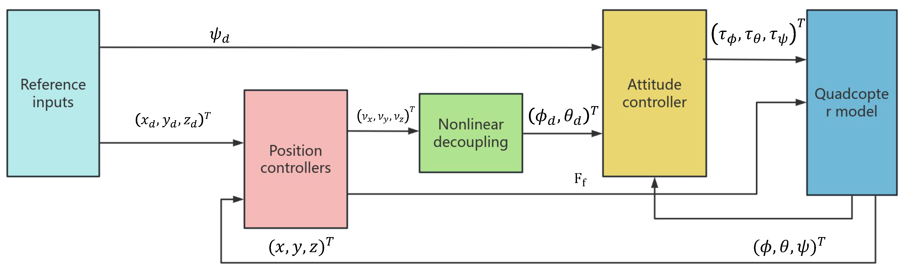
3. Flight Controller Design

This section focuses on the FOSM-ADRC method applied to quadrotor flight controller design. In addition, the propeller is very light compared to a brushless motor, and the moment of inertia induced by the propeller is neglected here.

The structure of the inner and outer loop structure control system designed in this paper is shown in Figure 2. The outer loop of the control system is the position controller, which adopts a PID controller; the inner loop is the attitude control, which adopts the FOSM-ADRC. The input to the position controller is the body position; the output is coupled to generate an attitude angle signal to the attitude controller, which generates an output to control the quadrotor body to track the reference input.

In the attitude controller design, the controller is divided into two inner and outer loops for control. In view of the good robustness and strong adaptability of the SMC as well as its fast response characteristics [20], a fractional-order reaching law sliding mode controller (FO-SMC) is used in the outer loop, and since we use a separate SMC alone, the control output oscillates at a higher frequency near the desired signal, which puts a higher demand on the quadrotor motor. In order to suppress this, the inner loop uses an ADRC, which can soften the output of the SMC and, at the same time, obtain a good anti-interference capability, which is a two-for-one approach. Figure 3 shows the control framework of this paper more visually.

Compared with the traditional single-loop PID controller, which is widely used in UAVs, the control structure proposed in this paper can achieve finer control accuracy and combine the strong robustness and anti-interference ability of both the SMC and ADRC to realize the stable operation of the quadrotor under strong interference conditions.

3.1. External Loop Controller (Fractional Order Convergence Law Smooth Mode Controller Design)

In the outer loop control part, in order to improve the corresponding speed of the controller, an SMC is selected to achieve a fast response, and it is designed for the attitude control system of the UAV. The tracking error of the attitude angle is first defined as follows:

$$\left(\begin{array}{c}{e}_{\varphi }\\ e_{\theta }\\ e_{\psi }\end{array}\right)=\left(\begin{array}{c}{\varphi }_d-\varphi \\ {\theta }_d-\theta \\ {\psi }_d-\psi \end{array}\right)$$

(2)

where $e_{\varphi },e_{\theta },e_{\psi }$ are the errors generated by subtracting the desired and actual values of roll angle, pitch angle, and yaw angle, respectively, which are obtained by taking the derivation of both sides of Equation (2) with respect to time t:

$$\left(\begin{array}{c}{\dot{e}}_{\varphi }\\ {\dot{e}}_{\theta }\\ {\dot{e}}_{\psi }\end{array}\right)=\left(\begin{array}{c}{\dot{\varphi }}_d-\dot{\varphi }\\ {\dot{\theta }}_d-\dot{\theta }\\ {\dot{\psi }}_d-\dot{\psi }\end{array}\right)$$

(3)

For the attitude ring, reference [21] designed a sliding mode surface as follows:

$$\begin{array}{c}\hfill \begin{array}{c}\hfill s_{\varphi }=c_{\varphi }\times ({\varphi }_d-\varphi )+({\dot{\varphi }}_d-\dot{\varphi })=c_{\varphi }\times e_{\varphi }+{\dot{e}}_{\varphi }\end{array}\end{array}$$

(4)

$$\begin{array}{c}\hfill \begin{array}{c}\hfill s_{\theta }=c_{\theta }\times ({\theta }_d-\theta )+({\dot{\theta }}_d-\dot{\theta })=c_{\theta }\times e_{\theta }+{\dot{e}}_{\theta }\end{array}\end{array}$$

(5)

$$\begin{array}{c}\hfill \begin{array}{c}\hfill s_{\psi }=c_{\psi }\times ({\psi }_d-\psi )+({\dot{\psi }}_d-\dot{\psi })=c_{\psi }\times e_{\psi }+{\dot{e}}_{\psi }\end{array}\end{array}$$

(6)

where the coefficients $c_{\varphi },c_{\theta },c_{\psi }$ are all positive constants. Both sides of the equation are obtained by derivation with respective to time t:

$$\begin{array}{c}\hfill \begin{array}{c}\hfill {\dot{s}}_{\varphi }=c_{\varphi }\times {\dot{e}}_{\varphi }+{\ddot{e}}_{\varphi }\end{array}\end{array}$$

(7)

$$\begin{array}{c}\hfill \begin{array}{c}\hfill {\dot{s}}_{\theta }=c_{\theta }\times {\dot{e}}_{\theta }+{\ddot{e}}_{\theta }\end{array}\end{array}$$

(8)

$$\begin{array}{c}\hfill \begin{array}{c}\hfill {\dot{s}}_{\psi }=c_{\psi }\times {\dot{e}}_{\psi }+{\ddot{e}}_{\psi }\end{array}\end{array}$$

(9)

Based on Equations (1) and (7)–(9), the quadrotor attitude loop SMC control law can be determined as follows:

$$\begin{array}{c}\hfill \begin{array}{c}\hfill u_2=I_x/l\left[C_{\varphi }({\dot{\varphi }}_d-\dot{\varphi }-{\dot{s}}_{\varphi }+{\ddot{\varphi }}_d)\right]-\dot{\theta }\dot{\psi }(I_y-I_z)/l-J_r\dot{\theta }{\mathrm{\Omega }}_r/l+K_4\dot{\varphi }\end{array}\end{array}$$

(10)

$$\begin{array}{c}\hfill \begin{array}{c}\hfill u_3=I_y/l\left[C_{\theta }({\dot{\theta }}_d-\dot{\theta }-{\dot{s}}_{\theta }+{\ddot{\theta }}_d)\right]-\dot{\varphi }\dot{\psi }(I_z-I_x)/l+J_r\dot{\varphi }{\mathrm{\Omega }}_r/l+K_5\dot{\theta }\end{array}\end{array}$$

(11)

$$\begin{array}{c}\hfill \begin{array}{c}\hfill u_4=I_z\left[C_{\psi }({\dot{\psi }}_d-\dot{\psi }-{\dot{s}}_{\psi }+{\ddot{\psi }}_d)\right]-\dot{\varphi }\dot{\theta }(I_x-I_y)+K_6\dot{\psi }\end{array}\end{array}$$

(12)

In terms of design reaching law, we use traditional reaching law, such as exponential reaching laws:

$$\begin{array}{c}\hfill \begin{array}{c}\hfill \dot{s}=-\epsilon \mathrm{sgn}s-ks\epsilon >0,k>0\end{array}\end{array}$$

(13)

where $\dot{s}=-ks$ is the exponential reaching term, which is solved by $s=s\left(0\right){\mathrm{e}}^{-kt}$. The rate of reaching depends on k, and the exponential term $-ks$ ensures that the system state reaches the sliding state at a large rate when s is large. The exponential reaching alone may not guarantee that the system state reaches the sliding mode surface in a finite time, so it is necessary to add an isovelocity reaching term $\dot{s}=-\epsilon sgn\left(s\right)$. That is, when the sliding mode variable s is close to 0, the reaching velocity is $\epsilon$ instead of 0. In order to better cut down the phenomenon of jitter, it is chosen to replace the sign function on the exponential reaching term with a hyperbolic tangent function and incorporate a fractional-order calculus operator.

The fractional-order calculus operator has the memory property, which ensures the influence of historical information on the present and future and helps to improve the quality of control. Compared with the traditional integer-order controller, it can describe the real object more accurately and adequately because of its fractional-order property while providing superior dynamic performance and robustness [22,23].

The hyperbolic tangent function is continuous and smooth, and the use of the hyperbolic correct function instead of the discontinuous sign function can effectively reduce the jitter in the sliding mode control. The hyperbolic tangent function is as follows:

$$\begin{array}{c}\hfill \begin{array}{c}\hfill \tanh \left({\displaystyle \frac{x}{\epsilon }}\right)={\displaystyle \frac{{\mathrm{e}}^{\frac{x}{\epsilon }}-{\mathrm{e}}^{-\frac{x}{\epsilon }}}{{\mathrm{e}}^{\frac{x}{ϵ}}+{\mathrm{e}}^{-\frac{x}{ϵ}}}}\end{array}\end{array}$$

(14)

where $ϵ>0$ and the magnitude of the $ϵ$ value determines how quickly or slowly the hyperbolic tangent function inflection point changes.

There are various forms of fractional-order calculus operators, of which the Caputo fractional-order calculus [24] is defined as

$$\begin{array}{c}\hfill \begin{array}{c}\hfill {}_{0}D_t^{\alpha }f\left(t\right)={\displaystyle \frac{1}{\mathrm{\Gamma }(n-\alpha )}}{\displaystyle {\mathit{\int }}_0^t}{\displaystyle \frac{f^{\left(n\right)}\left(\tau \right)}{{\left(t-\tau \right)}^{1-(n-\alpha )}}}d\tau \end{array}\end{array}$$

(15)

where $n-1\le \alpha <n$, n is a positive integer, and $\mathrm{\Gamma }(·)$ is the gamma function. Caputo fractional-order differentiation is the operation of nth order derivatives and then nth order integrals on a function.

Using Equations (14) and (15), the new hyperbolic tangent exponential reaching law for fractional order calculus is obtained as

$$\begin{array}{c}\hfill \begin{array}{c}\hfill {\dot{s}}_j=-{\epsilon }_j{(}_0{D}_t^{-\alpha }\tanh \left(s_j\right))-k_j{s}_j(j=\varphi ,\theta ,\psi )\end{array}\end{array}$$

(16)

where ${\epsilon }_j>0,k_j>0$ are adjustable parameters, ${}_{0}D_t^{-\alpha }$ is the fractional order differential integral operator, and $\alpha \in R, \alpha >0$ is the fractional order. The final fractional order reaching law sliding mode control law is obtained by replacing the sliding mode surface derivatives in the control law Equations (10)–(12) using the reaching law as

$$\begin{array}{c}\hfill \begin{array}{c}\hfill \left\{\begin{array}{cc}\hfill u_2& =I_x/l\left[C_{\varphi }({\dot{\varphi }}_d-\dot{\varphi }+{\epsilon }_{\varphi }{(}_0{D}_t^{-\alpha }\tanh \left(s_{\varphi }\right))+k_{\varphi }{s}_{\varphi }+{\ddot{\varphi }}_d)\right]-\dot{\theta }\dot{\psi }(I_y-I_z)/l\hfill \\ \hfill & - J_r\dot{\theta }{\mathrm{\Omega }}_r/l+K_4\dot{\varphi }\hfill \\ \hfill u_3& =I_y/l\left[C_{\theta }({\dot{\theta }}_d-\dot{\theta }+{\epsilon }_{\theta }{(}_0{D}_t^{-\alpha }\tanh \left(s_{\theta }\right))+k_{\theta }{s}_{\theta }+{\ddot{\theta }}_d)\right]-\dot{\varphi }\dot{\psi }(I_z-I_x)/l\hfill \\ \hfill & + J_r\dot{\varphi }{\mathrm{\Omega }}_r/l+K_5\dot{\theta }\hfill \\ \hfill u_4& =I_z\left[C_{\psi }({\dot{\psi }}_d-\dot{\psi }+-{\epsilon }_{\psi }{(}_0{D}_t^{-\alpha }\tanh \left(s_{\psi }\right))-k_{\psi }{s}_{\psi }+{\ddot{\psi }}_d)\right]-\dot{\varphi }\dot{\theta }(I_x-I_y)\hfill \\ \hfill & + K_6\dot{\psi }\hfill \end{array}\right.\end{array}\end{array}$$

(17)

• Stability analysis

Theorem 1. 

For the attitude angle model in the attitude angle control subsystem Equation (1), the controller Equation (17) can stabilize the controlled system in a finite amount of time for a given sliding mode surface, as described in Equations (4)–(6).

Proofs must be formatted as follows:

Proof of Theorem 1. 

For the sliding mode controller, the Lyapunov function is defined as

$$\begin{array}{c}\hfill \begin{array}{c}\hfill V_j={\displaystyle \frac{1}{2}}{s}_j^2(j=\varphi ,\theta ,\psi )\end{array}\end{array}$$

(18)

Carried over into Equations (3)–(12) and (20), we obtain

$$\begin{array}{c}\hfill \begin{array}{c}\hfill {\dot{V}}_j=s_j·{\dot{s}}_j=-{\epsilon }_j·s_j·{(}_0{D}_t^{-\alpha }\tanh \left(s_j\right))-k_j{s}_j^2\end{array}\end{array}$$

(19)

The hyperbolic tangent function $f\left(t\right)=tanh\left(s_j\right)$ is an odd function, continuous and smooth, and its value increases monotonically from −1 to 1 as $s_j$ increases. When $s_j$ decreases from a large positive value, the function starts to decrease from a value close to 1. $s_j$ decreases from a large positive value; the value of the function starts to decrease from a value close to 1. The fractional-order calculus operator ${}_{0}D_t^{-\alpha }$ takes into account the averaging effect of the hyperbolic tangent function over the integration interval $[0,t]$. If $s_j$ is always positive, even when it is decreasing, $f\left(t\right)$ is positive, only approaching 1 at a reduced rate, so the value of ${}_{0}D_t^{-\alpha }\tanh \left(s_j\right)$ remains positive, and the result of ${}_{0}D_t^{-\alpha }\tanh \left(s_j\right)$ becomes negative when $s_j$ decreases to a negative value, too. So, the first term ${\epsilon }_j·s_j·{(}_0{D}_t^{-\alpha }\tanh \left(s_j\right))$ value in Equation (21) will always be positive; then, the value of Equation (21) will always be negative, i.e., ${\dot{V}}_j<0$ is always valid, and therefore, the sliding mode Equations (4)–(6) can converge to 0 in finite time. Thus, it can be seen that $e_{\varphi },e_{\theta },e_{\psi }$ can converge to 0 in finite time. So, under the action of the controller Equation (17), the quadrotor attitude angle can be tracked to the desired trajectory angle in finite time. □

3.2. Inner Loop Controller (Active Disturbance Rejection Controller Design)

The conventional ADRC consists of a tracking differentiator (TD), an extended state observer ((ESO), and a nonlinear state error feedback (NLSEF). Its core components are disturbance estimation and dynamic compensation [25], as shown in Figure 2. The tracking differentiator arranges the transition process for the desired signal input to the control system, providing a trade-off between the overshoot of the system control and the fast response of the system control and reducing the overshoot of the control system caused by large changes in the given signal. The mathematical expression for the tracking differentiator for a second-order system is shown in Equation (20).

$$\begin{array}{c}\hfill \begin{array}{c}\hfill \left\{\begin{array}{c}\mathrm{fh}=\mathrm{fhan}(v_1\left(k\right)-v_d\left(k\right),v_2\left(k\right),r_0,h_0)\hfill \\ v_1(k+1)=v_1\left(k\right)+T·v_2\left(k\right)\hfill \\ v_2(k+1)=v_2\left(k\right)-T·\mathrm{fh}\hfill \end{array}\right.\end{array}\end{array}$$

(20)

where T is the sampling period of the control system and $v_1$ and $v_2$ are the system states. $v_d$ is the expected value of the system, and $\mathrm{fhan}(v_1,v_2,r_0,h_0)$ is the most rapid synthesis function, which is defined as shown in Equation (21):

$$\begin{array}{c}\hfill \begin{array}{c}\hfill \left\{\begin{array}{cc}& d=r_0{h}_0^2\hfill \\ & a_0=h_0{x}_2\hfill \\ & y=x_1+a_0\hfill \\ & a_1=\sqrt{d(d+8|y\left|\right)}\hfill \\ & a_2=a_0+{\displaystyle \frac{\mathrm{sign}\left(y\right)\left(a_1-d\right)}{2}}\hfill \\ & s_y={\displaystyle \frac{\mathrm{sign}(y+d)-\mathrm{sign}(y-d)}{2}}\hfill \\ & a=\left(a_0+y-a_2\right)s_y+a_2\hfill \\ & s_a={\displaystyle \frac{\mathrm{sign}(a+d)-\mathrm{sign}(a-d)}{2}}\hfill \\ & \mathrm{fhan}=-r[{\displaystyle \frac{a}{d}}-\mathrm{sign}\left(a\right)]s_a-r_0\mathrm{sign}\left(a\right)\hfill \end{array}\right.\end{array}\end{array}$$

(21)

where $r_0$ and $h_0$ are adjustable parameters related to the tracking performance, where $r_0$ is the speed factor. Increasing $r_0$ speeds up the response and reduces the transition process, but too large a value of $r_0$ makes the tracking signal close to the desired input signal and loses the significance of the transition process. $h_0$ is the filtering factor; increasing the value of $h_0$ value can improve the filtering effect but produces phase delay. $sign\left(x\right)$ is the sign function.

ESO takes the input and output variables of the control system as the inputs of the observer and adopts a nonlinear combination to observe the disturbances of the system, expanding a new state variable on top of the original state variable of the system, which is regarded as the total disturbance variable. ESO does not need the mathematical model of the controlled object [26] and only estimates the total disturbances of the system based on the system’s inputs and outputs. The total disturbance of the system is estimated and compensated to the controller, which is the core part of ADRC; the mathematical expression of ESO is shown in Equation (22):

$$\begin{array}{c}\hfill \begin{array}{c}\hfill \left\{\begin{array}{cc}\hfill {\epsilon }_1& =z_1\left(k\right)-y\left(k\right)\hfill \\ \hfill z_1(k+1)& =z_1\left(k\right)+T\left[z_2\left(k\right)-{\beta }_{01}{\epsilon }_1\right]\hfill \\ \hfill z_2(k+1)& =z_2\left(k\right)+T\left[z_3\left(k\right)-{\beta }_{02}\mathrm{fal}\left({\epsilon }_1,{\alpha }_1,\delta \right)+bu\right]\hfill \\ \hfill z_3(k+1)& =z_3\left(k\right)-T{\beta }_{03}\mathrm{fal}\left({\epsilon }_1,{\alpha }_2,\delta \right)\hfill \end{array}\right.\end{array}\end{array}$$

(22)

where $\mathrm{fal}(x,\alpha ,\delta )$ is a nonlinear function defined as shown in Equation (23):

$$\begin{array}{c}\hfill \begin{array}{c}\hfill \mathrm{fal}(x,\alpha ,\delta )=\left\{\begin{array}{cc}{\displaystyle \frac{x}{{\delta }^{(1-\alpha )}}},\hfill & \left|x\right|\le \delta \hfill \\ \mathrm{sign}\left(x\right)|x{|}^{\alpha },\hfill & \left|x\right|>\delta \hfill \end{array}\right.\end{array}\end{array}$$

(23)

where $\delta$ is a constant that affects the filtering effect and $\alpha$ is an adjustment parameter for the length of the nonlinear interval of the function number. ${\alpha }_1,{\alpha }_2$ is a variable parameter related to the nonlinear interval of the $\mathrm{fal}(x,\alpha ,\delta )$ function, which is generally taken as ${\alpha }_1=0.5,{\alpha }_2=0.25$; ${\beta }_{01},{\beta }_{02},{\beta }_{03}$ are determined by the sampling step of the system.

The mathematical expression of the Nonlinear State Error Feedback Control Law (NLSEF) is shown in Equation (24), which utilizes the tracking signals generated in the TD stage and the observation signals generated in the ESO stage, calculates the tracking error of the system, and finally generates the control quantities by means of a nonlinear combination:

$$\begin{array}{c}\hfill \begin{array}{c}\hfill \left\{\begin{array}{c}{e}_1=v_1\left(k\right)-z_1\left(k\right)\hfill \\ e_2=v_2\left(k\right)-z_2\left(k\right)\hfill \\ u_0=\mathrm{fhan}(e_1,c{e}_2,r,h_1)\hfill \end{array}\right.\end{array}\end{array}$$

(24)

where r is the control volume gain, which generally takes a larger value; c is the damping factor; and $h_1$ is the accuracy factor. Finally, the control volume can be obtained by compensating the state variables of the expansion observed by the ESO, i.e., eliminating the total perturbation variables, as in Equation (25), where $b_0$ is the compensation factor, which should be close to the actual value of the model [27].

$$\begin{array}{c}\hfill \begin{array}{c}\hfill u={\displaystyle \frac{u_0-z_3}{b_0}}\end{array}\end{array}$$

(25)

4. Experiments and Results

This section presents the dynamics model of the UAV in Equation (1) used to test the performance of the proposed control method. The hardware environment in the simulation environment was an Intel(R) Xeon(R) W-2145 CPU 16-core processor, Windows 10 system. In addition, the performance of the proposed controller was demonstrated by comparing it with an ordinary SMC as well as FO-SMC. In Section 3, we present the details of the design of the proposed controller and the design of the common SMC. The detailed parameters in the simulation control are shown in

Table 2. FO-SMC parameters.

	${\mathit{k}}_{\mathit{j}}(\mathit{j}=\mathit{\varphi },\mathit{\theta },\mathit{\psi })$	${\mathit{c}}_{\mathit{j}}(\mathit{j}=\mathit{\varphi },\mathit{\theta },\mathit{\psi })$	${\mathit{\alpha }}_{\mathit{j}}(\mathit{j}=\mathit{\varphi },\mathit{\theta },\mathit{\psi })$	${\mathit{\epsilon }}_{\mathit{j}}(\mathit{j}=\mathit{\varphi },\mathit{\theta },\mathit{\psi })$
$\varphi$	7	0.95	0.5	0.01
$\theta$	7.5	0.95	0.5	0.01
$\psi$	6.8	1	0.5	0.0055

and

Table 3. ADRC parameters.

	${\mathit{K}}_{\mathit{p}}$	${\mathit{K}}_{\mathit{i}}$	${\mathit{K}}_{\mathit{d}}$	${\mathit{\beta }}_1$	${\mathit{\beta }}_2$	${\mathit{b}}_0$
$\varphi$	0.1	0.1	0.003	500	1800	300
$\theta$	0.1	0.1	0.003	500	1800	300
$\psi$	0.15	0.2	0.001	350	1400	200

.

The simulation experiments were mainly carried out using the FOSM-ADRC, ordinary SMC, and FO-SMC proposed in this paper. The simulation experiment platform used Firmament (FMT), a project developed and open-sourced by AMOVLAB [19], which is a model-based design (MBD) open-source driver. The simulation project was divided into three main parts: (1) The embedded software framework for flight control contains the core software of the flight control, driver, and function modules. (2) The flight control algorithm model framework contains the algorithm model based on Matlab/Simulink (version:R2022b), such as navigation, control, state machine, controlled object model, etc. The algorithm model can be generated by automatic code generation. The algorithm model can be merged into FMT-FW through automatic code generation, thus constituting the complete flight control system software. (3) The 3D engine realizes the simulation environment, providing realistic rendering effects and rich simulation scenes.

The quadrotor flight task in the simulation was set to take off and fly along the X-axis for 10 m in 5 s at an altitude of 10 m and fly steadily in a stable position until the beginning of 40 s to execute the landing command. The experimental environment was divided into three cases of simulation: (1) no interference signal added to the simulation; (2) a weak white noise obeying normal distribution added to the simulation to simulate a weak interference signal; and (3) a strong white noise obeying normal distribution added to the simulation to simulate a strong interference signal.

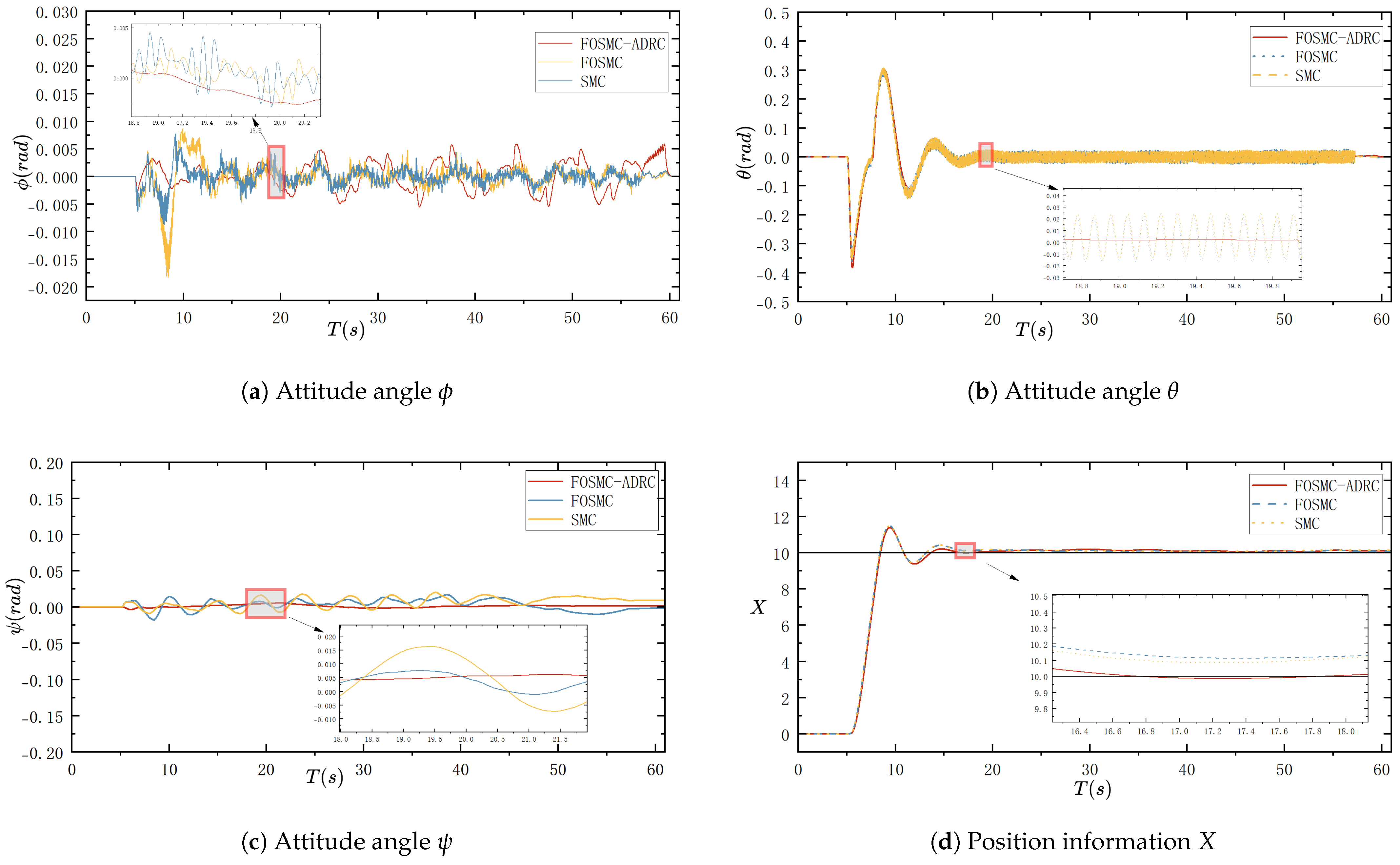
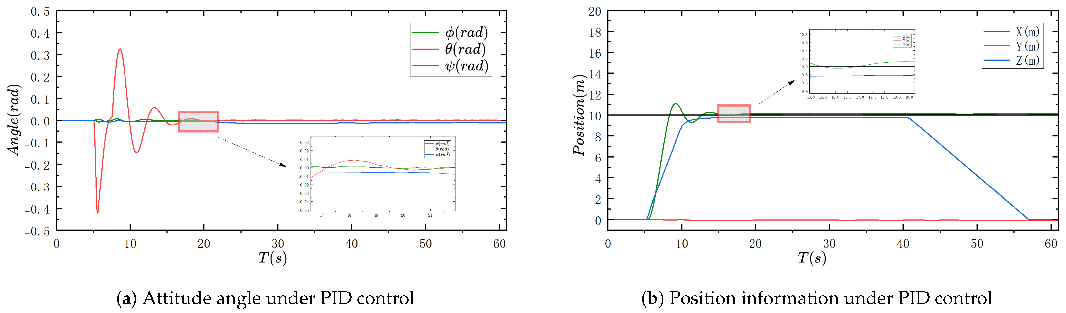
4.1. Analysis of Experimental Results Without Interference

The simulation effect of the controller controlling the attitude angle, as well as the position information without interference, is shown in Figure 4a–f.

Figure 4a–c show the attitude angles in the resultant graphs, where the proposed controller suppresses the high-frequency switching oscillations of the output of the SMC well, which makes the output smoother and more stable and has a higher control accuracy in the attitude angle $\psi$. And, the control accuracy is higher in the attitude angle $\psi$. Figure 4d–f of the total position information show that all three algorithms can track the desired value in a finite time and the tracking effect is better. A more visual comparison can be made by referring to the steady-state error table (

Table 4. Steady-state error.

	$\mathit{\varphi }$ (rad)	$\mathit{\theta }$ (rad)	$\mathit{\psi }$ (rad)
FOSM-ADRC	0.00108	0.0205	0.0018
FOSMC	0.00141	0.02734	0.00615
SMC	0.00105	0.02747	0.0078

); the controller proposed in this paper has a higher control accuracy, and the response speed in the altitude channel results in a certain degree of improvement compared with the other two kinds of controllers.

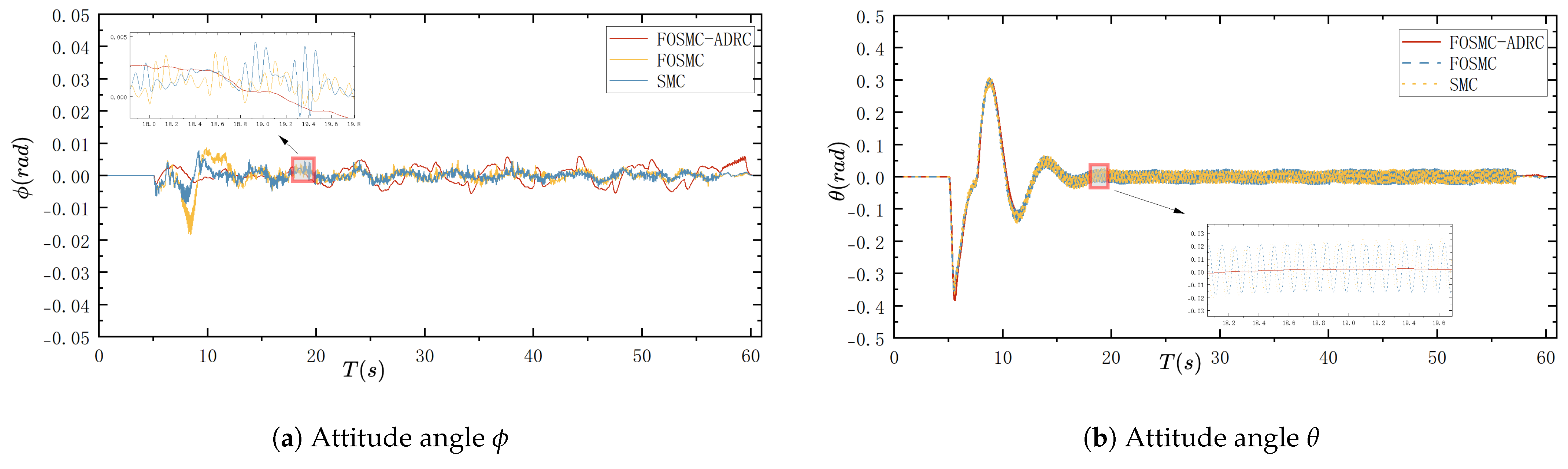
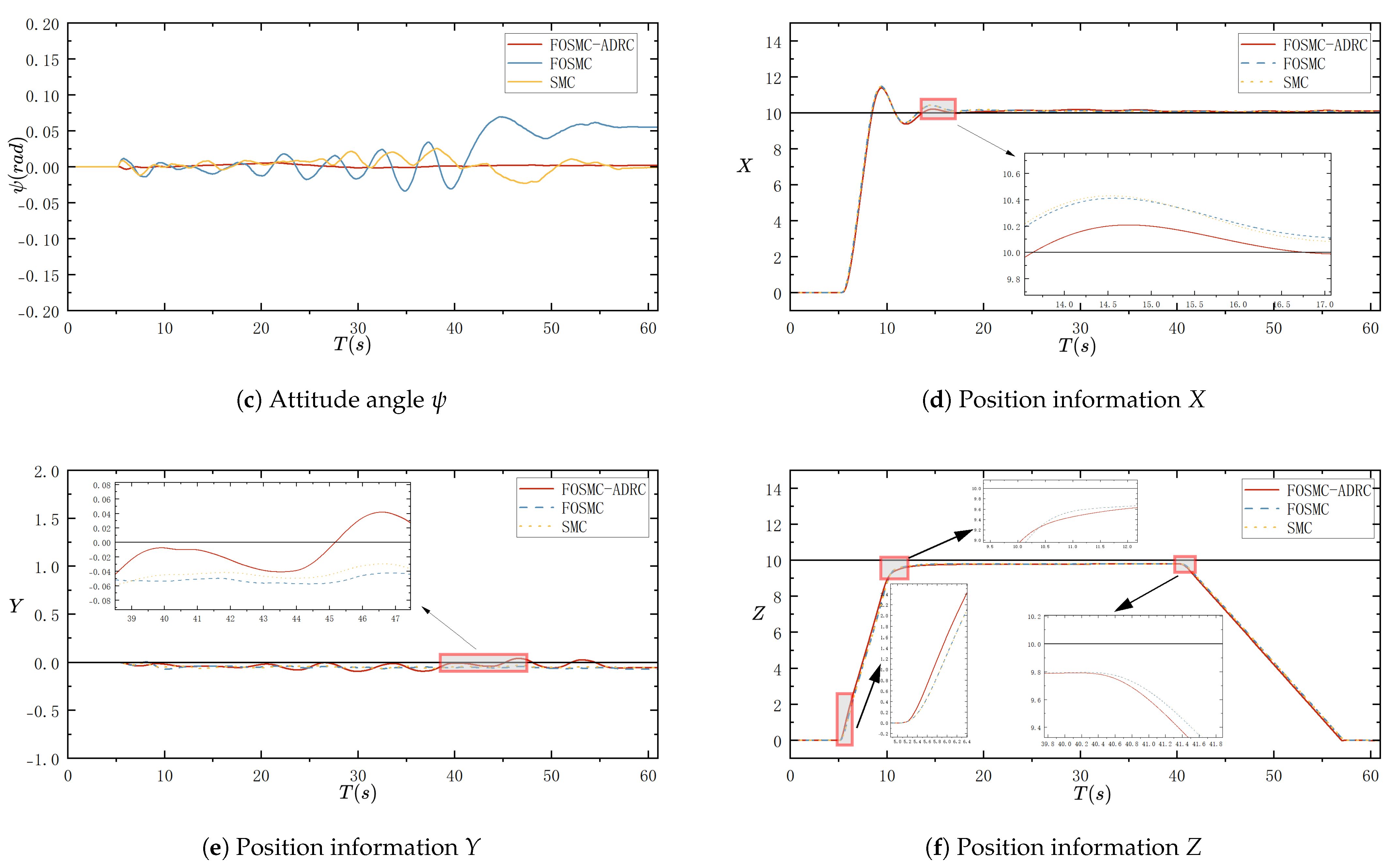
4.2. Analysis of Experimental Results in Case of Weak Interference

The simulation effect of adding the weak interference, where the controller controls the attitude angle as well as the position information, is shown in Figure 5a–f.

Figure 5a–f show the attitude angle and position information results in the three controllers in the weak interference in the experimental situation, during which they can work normally, and in the absence of interference in the three controllers, the control effect is similar and did not occur in a large change. The next step should be to further increase the interference lightness to observe whether there is a large change in the difference in the control effect of the three controllers.

4.3. Analysis of Experimental Results in Case of Strong Interference

The simulation effect of adding the controller to control the attitude angle, as well as the position information, in the case of strong interference is shown in Figure 6a–f.

Figure 6a–f show the attitude angle and position information results. The three controllers revealed a large difference. In the attitude angle graph, this can be seen very intuitively. Compared with the addition of the weak interference, with the addition of the strong interference, the UAV with the three different controllers is affected. The SMC and the FO-SMC receive a more serious impact in the attitude angle graph, while the FOSM-ADRC proposed in this paper is also affected, but the attitude angle control is relatively stable, and no divergence occurs. In the position diagrams, the comparison of the control effect of the three controllers is more obvious, especially in the Z-axis diagram in Figure 6f, where the larger vibrations of the SMC and the FO-SMC occur in the undispersed stage, but the FOSM-ADRC proposed in this paper is still relatively stable. Overall, the normal SMC loses control at about 24 s and disperses immediately, and although the FO-SMC also loses control at a similar time, it shows some signs of retracing within a short period and exhibits a faster response speed and a stronger anti-interference capability compared to the normal SMC. In addition, the FOSM-ADRC proposed in this paper is still relatively stable in this strong interference situation. Only in the simulation image, there is a little jitter, but it never loses control, and there is no dispersion, so it can be seen that the controller proposed in this paper exhibits strong anti-interference performance.

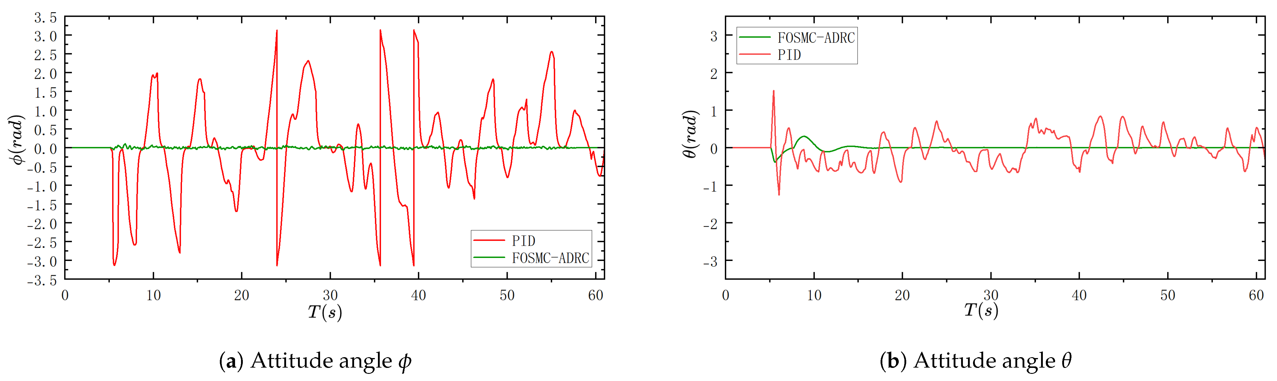
4.4. Analysis of Comparative Experiments of FOSM-ADRC and PID in Case of Strong Interference

In order to make the performance of this controller persuasive, a conventional PID controller was designed to serve as a comparison. As shown in Figure 7, the PID controller is able to control the quadrotor in flight normally under the parameters (

Table 5. PID Parameters.

	${\mathit{K}}_{\mathit{p}}$	${\mathit{K}}_{\mathit{i}}$	${\mathit{K}}_{\mathit{d}}$
$\varphi$	0.1	0.1	0.003
$\theta$	0.1	0.1	0.003
$\psi$	0.1	0.1	0.0015

) in a disturbance-free environment.

In the case of the same controller parameters, we add the same strong interference signal to the model as before, as shown in Figure 8. The PID controller and the controller proposed in this paper as a comparison can be clearly seen. In the initial moment, the PID controller in the attitude angle control has been dispersed and cannot form an effective control of the quadrotor. In the three graphs of position information, it is obvious that the quadrotor is not under control.

It can be seen that the controller proposed in this paper has a certain degree of anti-interference ability, and its anti-interference ability in the simulation experiments is more powerful than that of the traditional SMC and traditional PID controller.

Combining the above experimental results, the FOSM-ADRC proposed in this paper can operate stably in the case of no interference, and in the case of strong interference, it has a stronger anti-interference ability and more robustness compared with other comparative controllers. While obtaining superior performance, the more limited point is that the controller requires more parameters, and the process of adjusting the parameters is tedious, which needs to be addressed in the future.

5. Conclusions

In this paper, the attitude controller was designed with the quadrotor attitude angle as the control object, and some series of simulation experiments were carried out. The main conclusions are as follows: (1) Finite-time convergence. By adopting the FOSM-ADRC method, the designed quadrotor unmanned aerial vehicle (UAV) attitude controller successfully solves the problem of the convergence of the control variables in a finite time. This was verified by simulations in the Matlab/Simulink (version:R2022b) environment, showing that the controller was able to respond quickly and reach a steady state within a predetermined time. (2) High-frequency vibration suppression. The simulation results further confirm that the controller can effectively suppress the high-frequency vibration of the output. This is critical for improving system stability and reducing errors caused by vibration, especially when operating at high speeds or in complex environments. (3) Anti-interference capability. The designed controller exhibits enhanced anti-interference capability compared to ordinary sliding mode control (SMC) and PID controllers. This enhanced robustness allows the controller to maintain performance stability and reliability in the face of external perturbations and system uncertainties. (4) Comprehensive efficacy. In summary, the simulation results show that the controller not only successfully suppresses the high-frequency jitter in the output of the common sliding mode controller but also achieves strong anti-interference capability. These characteristics make the FOSM-ADRC method have significant application potential and advantages in the field of quadrotor UAV attitude control. Future research can further explore the performance of the FOSM-ADRC method under different types of UAVs and a wider range of operating conditions, as well as explore how to further optimize the controller parameters in order to improve the system’s responsiveness and stability, e.g., by using intelligent algorithms to automatically regulate the parameters or by reducing the regulated parameters while guaranteeing the control performance, among other aspects.

References

1. Guo, Y.; Jiang, B.; Zhang, Y. A novel robust attitude control for quadrotor aircraft subject to actuator faults and wind gusts. IEEE/CAA J. Autom. Sin. 2017, 5, 292–300. [Google Scholar] [CrossRef]
2. Mahony, R.; Kumar, V.; Corke, P. Multirotor aerial vehicles: Modeling, estimation, and control of quadrotor. IEEE Robot. Autom. Mag. 2012, 19, 20–32. [Google Scholar] [CrossRef]
3. Noordin, A.; Mohd Basri, M.A.; Mohamed, Z.; Mat Lazim, I. Adaptive PID Controller Using Sliding Mode Control Approaches for Quadrotor UAV Attitude and Position Stabilization. Arab. J. Sci. Eng. 2021, 46, 963–981. [Google Scholar] [CrossRef]
4. Elkhatem, A.S.; Engin, S.N. Robust LQR and LQR-PI control strategies based on adaptive weighting matrix selection for a UAV position and attitude tracking control. Alex. Eng. J. 2022, 61, 6275–6292. [Google Scholar] [CrossRef]
5. Lopez, J.; Dormido, R.; Dormido, S.; Gomez, J.P. A robust H∞ controller for an UAV flight control system. Sci. World J. 2015, 2015, 403236. [Google Scholar] [CrossRef]
6. Baek, J.; Jin, M.; Han, S. A new adaptive sliding-mode control scheme for application to robot manipulators. IEEE Trans. Ind. Electron. 2016, 63, 3628–3637. [Google Scholar] [CrossRef]
7. Wang, J.; Alattas, K.A.; Bouteraa, Y.; Mofid, O.; Mobayen, S. Adaptive finite-time backstepping control tracker for quadrotor UAV with model uncertainty and external disturbance. Aerosp. Sci. Technol. 2023, 133, 108088. [Google Scholar] [CrossRef]
8. Gao, B.; Liu, Y.-J.; Liu, L. Adaptive neural fault-tolerant control of a quadrotor UAV via fast terminal sliding mode. Aerosp. Sci. Technol. 2022, 129, 107818. [Google Scholar] [CrossRef]
9. Nguyen, S.D.; Lam, B.D.; Ngo, V.H. Fractional-order sliding-mode controller for semi-active vehicle MRD suspensions. Nonlinear Dyn. 2020, 101, 795–821. [Google Scholar] [CrossRef]
10. Han, J. From PID to active disturbance rejection control. IEEE Trans. Ind. Electron. 2009, 56, 900–906. [Google Scholar] [CrossRef]
11. Wang, S.; Chen, J.; He, X. An adaptive composite disturbance rejection for attitude control of the agricultural quadrotor UAV. ISA Trans. 2022, 129, 564–579. [Google Scholar] [CrossRef] [PubMed]
12. Ran, M.; Wang, Q.; Dong, C.; Xie, L. Active disturbance rejection control for uncertain time-delay nonlinear systems. Automatica 2020, 112, 108692. [Google Scholar] [CrossRef]
13. Zhu, E.; Pang, J.; Sun, N.; Gao, H.; Sun, Q.; Chen, Z. Airship horizontal trajectory tracking control based on active disturbance rejection control (ADRC). Nonlinear Dyn. 2014, 75, 725–734. [Google Scholar] [CrossRef]
14. Li, B.; Gong, W.; Yang, Y.; Xiao, B.; Ran, D. Appointed Fixed Time Observer-Based Sliding Mode Control for a Quadrotor UAV Under External Disturbances. IEEE Trans. Aerosp. Electron. Syst. 2022, 58, 290–303. [Google Scholar] [CrossRef]
15. Xu, L.-X.; Ma, H.-J.; Guo, D.; Xie, A.-H.; Song, D.-L. Backstepping Sliding-Mode and Cascade Active Disturbance Rejection Control for a Quadrotor UAV. IEEE/ASME Trans. Mechatron. 2020, 25, 2743–2753. [Google Scholar] [CrossRef]
16. Quan, Q. Introduction to Multicopter Design and Control; Springer: Berlin/Heidelberg, Germany, 2017. [Google Scholar]
17. Xiong, J.-J.; Zhang, G. Discrete-time sliding mode control for a quadrotor UAV. Optik 2016, 127, 3718–3722. [Google Scholar] [CrossRef]
18. Xiong, J.-J.; Zheng, E.-H. Position and attitude tracking control for a quadrotor UAV. ISA Trans. 2014, 53, 725–731. [Google Scholar] [CrossRef]
19. JcZou. Firmament-Autopilot/FMT-Firmware. GitHub Repository. 2024. Available online: https://github.com/Firmament-Autopilot/FMT-Firmware (accessed on 29 September 2024).
20. Liu, Y.; Wang, Z.; Xiong, L.; Wang, J.; Jiang, X.; Bai, G.; Li, R.; Liu, S. DFIG wind turbine sliding mode control with exponential reaching law under variable wind speed. Int. J. Electr. Power Energy Syst. 2018, 96, 253–260. [Google Scholar] [CrossRef]
21. Xiong, J.-J.; Zhang, G.-B. Global fast dynamic terminal sliding mode control for a quadrotor UAV. ISA Trans. 2017, 66, 233–240. [Google Scholar] [CrossRef]
22. Diethelm, K.; Ford, N.J.; Freed, A.D. A predictor-corrector approach for the numerical solution of fractional differential equations. Nonlinear Dyn. 2002, 29, 3–22. [Google Scholar] [CrossRef]
23. Yang, N.; Liu, C. A novel fractional-order hyperchaotic system stabilization via fractional sliding-mode control. Nonlinear Dyn. 2013, 74, 721–732. [Google Scholar] [CrossRef]
24. Odibat, Z. Approximations of fractional integrals and Caputo fractional derivatives. Appl. Math. Comput. 2006, 178, 527–533. [Google Scholar] [CrossRef]
25. Zhao, L.; Dai, L.W.; Xia, Y.Q.; Li, P. Attitude control for quadrotors subjected to wind disturbances via active disturbance rejection control and integral sliding mode control. Mech. Syst. Signal Process. 2019, 129, 531–545. [Google Scholar] [CrossRef]
26. Wang, Z.; Zhao, T. Based on robust sliding mode and linear active disturbance rejection control for attitude of quadrotor load UAV. Nonlinear Dyn. 2022, 108, 3485–3503. [Google Scholar] [CrossRef]
27. Yin, Z.; Du, C.; Liu, J.; Sun, X.; Zhong, Y. Research on autodisturbance-rejection control of induction motors based on an ant colony optimization algorithm. IEEE Trans. Ind. Electron. 2017, 65, 3077–3094. [Google Scholar] [CrossRef]
Figure 1. Quadrotor-UAV.
Applsci 15 00556 g001
Figure 2. Control system structure diagram.
Applsci 15 00556 g002
Figure 3. The proposed controller framework.
Applsci 15 00556 g003
Figure 4. Experimental results without interference.
Applsci 15 00556 g004aApplsci 15 00556 g004b
Figure 5. Experimental results with weak interference.
Applsci 15 00556 g005aApplsci 15 00556 g005b
Figure 6. Experimental results with strong interference.
Applsci 15 00556 g006aApplsci 15 00556 g006b
Figure 7. Experimental results with strong interference.
Applsci 15 00556 g007
Figure 8. Experimental results of PID and FOSM-ADRC with strong interference.
Applsci 15 00556 g008aApplsci 15 00556 g008b