Enhancing Deepfake Detection Through Quantum Transfer Learning and Class-Attention Vision Transformer Architecture

Abstract

The widespread use of the internet, coupled with the increasing production of digital content, has caused significant challenges in information security and manipulation. Deepfake detection has become a critical research topic in both academic and practical domains, as it involves identifying forged elements in artificially generated videos using various deep learning and artificial intelligence techniques. In this dissertation, an innovative model was developed for detecting deepfake videos by combining the Quantum Transfer Learning (QTL) and Class-Attention Vision Transformer (CaiT) architectures. The Deepfake Detection Challenge (DFDC) dataset was used for training, and a system capable of detecting spatiotemporal inconsistencies was constructed by integrating QTL and CaiT technologies. In addition to existing preprocessing methods in the literature, a novel preprocessing function tailored to the requirements of deep learning models was developed for the dataset. The advantages of quantum computing offered by QTL were merged with the global feature extraction capabilities of the CaiT. The results demonstrated that the proposed method achieved a remarkable performance in detecting deepfake videos, with an accuracy of 90% and ROC AUC score of 0.94 achieved. The model’s performance was compared with other methods evaluated on the DFDC dataset, highlighting its efficiency in resource utilization and overall effectiveness. The findings reveal that the proposed QTL-CaiT-based system provides a strong foundation for deepfake detection and contributes significantly to the academic literature. Future research should focus on testing the model on real quantum devices and applying it to larger datasets to further enhance its applicability.

1. Introduction

Deep learning, a subfield of artificial intelligence, began its foundational development in the 1950s and has gained significant momentum in recent years due to the increasing availability of data and advancements in hardware technology. Neural networks with deeper layers have enabled effective modeling of complex datasets, achieving results that surpass human capabilities in areas like image processing, natural language processing, and autonomous systems. These advancements have positioned deep learning at the forefront of artificial intelligence research and technological innovation.

Deepfakes, a specific application of deep learning, have emerged as a critical concern due to their potential to disseminate misinformation and undermine democratic processes. By integrating fake facial elements into real footage, these technologies can create highly convincing manipulated videos. Initially popularized in entertainment, deepfakes have raised significant concerns for journalism and public trust when used maliciously in misinformation campaigns [1].

Deep learning techniques such as Convolutional Neural Networks (CNNs) and Generative Adversarial Networks (GANs) are essential for both the creation and detection of fake videos. Detection efforts often rely on identifying spatial and temporal inconsistencies, such as unnatural blinking patterns or misaligned facial movements [2].

However, despite their effectiveness, current methods face significant challenges, including the need for real-time detection systems, limited dataset diversity, and the rapid evolution of deepfake generation techniques. Although many approaches perform well in controlled settings, their applicability in real-world scenarios remains limited, highlighting the need for more robust solutions [3].

Quantum computing, leveraging quantum bits (qubits), offers transformative capabilities for solving complex problems beyond the reach of classical systems. By utilizing principles such as superposition and entanglement, quantum systems have potential applications in fields ranging from material science to cryptography and drug discovery. Quantum computing’s integration with artificial intelligence has given rise to quantum machine learning (QML), enabling more efficient data processing and innovative algorithm development [4].

Quantum machine learning combines classical machine learning techniques with quantum computational advantages to enhance the processing of high-dimensional data. Tools such as Parametric Quantum Circuits (PQCs) address classical computational limitations, offering novel solutions for emerging AI challenges [5].

In the literature, several significant studies have been conducted to improve deepfake detection. Han et al. (2024) developed a model for video-based deepfake detection guided by facial feature adaptation. Based on the CLIP model, this method achieved a 0.9% AUROC improvement in cross-dataset evaluations and a 4.4% accuracy increase on the DFDC dataset. The study demonstrated consistent performance in deepfake detection by optimizing foundational models based on facial features [6].

Guarnera et al. (2020) introduced an innovative model based on convolutional traces aimed at detecting manipulated images. By utilizing convolutional features for facial data analysis, this method achieved an accuracy of 87%. The study presented a simple yet effective approach for forgery detection [7].

Zhao et al. (2021) developed a deepfake detection model based on multi-attention mechanisms. This model was tested across various datasets, achieving 89.5% accuracy and a 0.92 AUROC. The study successfully highlighted the impact of attention mechanisms in deepfake detection [8].

Zhou et al. (2021) designed a deepfake detection method combining visual and audio data. By integrating visual and audio analyses using the ResNet and Swin Transformer architectures, this approach achieved 92.1% accuracy on the DFDC dataset, offering an effective solution for deepfake detection [9].

Thing et al. (2023) compared the effects of CNNs and Transformer architectures in deepfake detection. Using ResNet and Swin Transformer models, they achieved 92.02% accuracy and a 97.61% AUC on the DFDC dataset. The study analyzed the advantages of both architectures and their performances on different datasets [10].

Saikia et al. (2021) proposed a hybrid CNN-LSTM model for video-based deepfake detection leveraging optical flow features. By combining the spatial awareness of CNNs with the temporal analysis capabilities of LSTMs, this model achieved 66.26% accuracy on the DFDC dataset, demonstrating its effectiveness [11].

Wodajo et al. (2020) focused on detecting deepfake videos using Convolutional Vision Transformer (CViT). This model achieved 91.5% accuracy and a 0.91 AUROC on the DFDC dataset by analyzing facial regions in detail. Despite its high accuracy, the model’s intensive resource usage limits its applicability to constrained systems [12].

While existing deepfake detection methods have achieved significant success in the literature, they also possess certain limitations. Studies have revealed that these methods often rely heavily on specific datasets and focus on superficial features of fake videos [13]. Despite the effectiveness of deep learning-based models in forgery detection, their generalization capabilities have been observed to falter when faced with more complex and advanced deepfake technologies [14]. For example, while some models achieve high accuracy in specific scenarios, their performance tends to decline on broader and more diversified datasets [15]. Additionally, advanced detection techniques that address the dynamic and temporal structures of deepfake videos are still limited in number [16]. These studies in the literature emphasize a critical need for the development of more comprehensive and robust algorithms.

This thesis proposes the integration of QTL and Vision Transformer (ViT) technologies. By combining these two powerful technologies, the aim is to achieve higher accuracy and performance in deepfake detection. By merging the computational advantages of QTL with ViT’s deep image processing capabilities, the model seeks to more precisely identify spatial and temporal inconsistencies. Specifically, ViT’s ability to learn global features of images facilitates the detection of fine details in manipulated videos, bringing a new dimension to deepfake detection. This approach aims to provide a unique contribution to the existing literature by addressing its gaps and shedding light on the more complex dimensions of deepfake technologies.

2. Materials and Methods

This section provides detailed information regarding the conducted study.

2.1. Model Summary

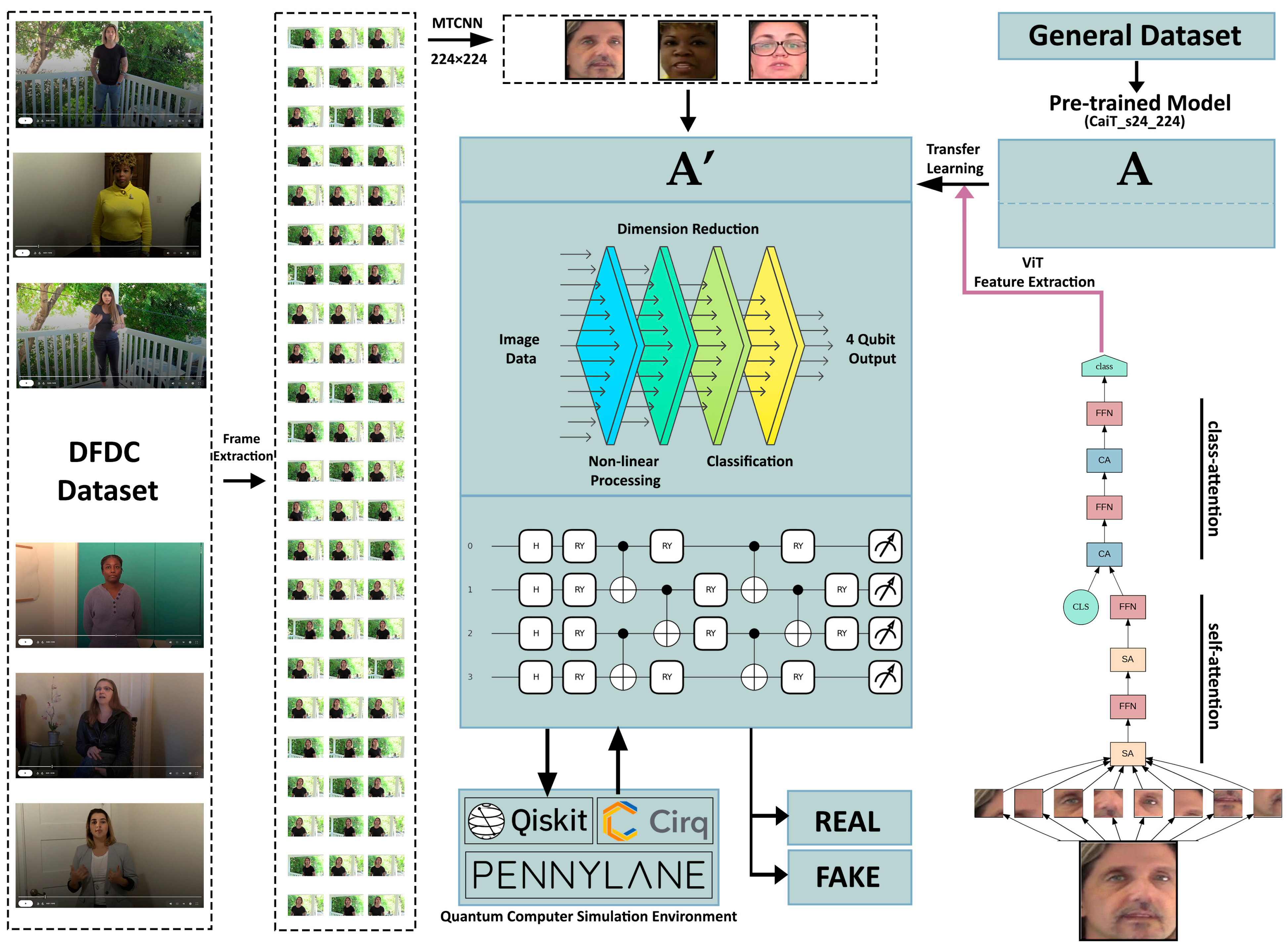
The proposed model for detecting deepfake videos, utilizing the DFDC dataset [17,18], begins its process by splitting videos into frames. At this stage, videos are transformed into an analyzable format, making each frame suitable for deepfake detection. Frame extraction ensures consistent and structured data acquisition from videos. Subsequently, these frames undergo face detection using the Multi-task Cascaded Convolutional Network (MTCNN) algorithm, and their dimensions are resized to 224 × 224 pixels. This preprocessing step standardizes input data for the model, aiming to enhance both accuracy and processing efficiency. The processed frames are prepared for the feature extraction phase.

During feature extraction, the images are processed through a ViT-based model, specifically the CaiT. The CaiT effectively captures both global and local features of the images through self-attention and class-attention mechanisms, offering advanced hierarchical representations. This phase generates the fundamental data required for deepfake detection. The layer structure and processing steps of the CaiT enhance the model’s strong feature extraction capabilities. The extracted features are subsequently fed into a Quantum Neural Network (QNN) model, operating with quantum simulation tools like Qiskit, PennyLane, and Cirq. Using quantum gates (Hadamard, RY, CX), this analysis enables advanced computations for deepfake detection.

In the final stage, the model classifies the analyzed images as either “Real” or “Fake”. This process combines the feature extraction capability of the CaiT with the analytical power of a QNN to achieve higher accuracy rates. The steps and operations of the model are illustrated in detail in Figure 1 as a flowchart.

2.2. Dataset and Model Parameters

Deepfake detection requires comprehensive analyses and enhanced generalization capabilities. To achieve this, two datasets were utilized: the DFDC dataset and the Deepfake and Real Images Dataset available on Kaggle. These datasets provide the diversity and quality needed for identifying fake and real content, enabling the model to perform effectively under various conditions.

The DFDC dataset, developed by Facebook in 2019, was released to support research into deepfake detection. It includes thousands of video files labeled as real or fake, featuring diverse facial characteristics, expressions, and angles. These attributes make the DFDC dataset ideal for training and validating deepfake detection models. The dataset serves as a comprehensive resource for researchers analyzing the impact of variables like facial expressions, angles, and lighting on deepfake detection [17].

The Deepfake and Real Images Dataset, hosted on Kaggle, consists of deepfake and real images created under various scenarios. This dataset focuses on still-image-based deepfake detection. It offers a wide range of visual variations and is essential for training, validation, and testing processes. With images generated using different algorithms, this dataset plays a significant role in training models for image-based deepfake detection [19].

Together, these datasets provide the model with a broad perspective and enhance its ability to generalize across different data types, ensuring effective performance in complex tasks like deepfake detection.

The parameters used during model training were defined considering the constraints of the Google Colab environment, dataset size, and hardware limitations, such as the large video file sizes and the need for efficient preprocessing to handle diverse data types. This study was conducted on a CPU with high RAM settings in the Google Colab environment. GPU utilization was avoided due to high costs, and the training process had to be efficiently structured since a Colab session could remain active for a maximum of 24 h. This limited runtime posed challenges, especially when working with large datasets.

The training process was conducted on the Google Colab platform, which, even in its premium version, restricts session durations to a maximum of 24 h. Although the dataset contains approximately 100,000 videos, only 45,000 videos could be processed due to these time limitations. Each video requires an average of 4 min for training, resulting in a total of 180,000 min (or 3000 h) to complete the entire dataset. Given these constraints, completing even a single epoch within the available session time was practically impossible.

To address this limitation, the model was designed to save its state after every two videos, ensuring that training could be resumed from the last processed video in subsequent sessions. Consequently, an epoch count of 1 was selected as a “representative value” to demonstrate the feasibility of the training process and provide initial performance insights.

For further details regarding the training process and the model’s save strategy, please refer to Section 2.10. The batch size, which defines how many samples are processed in each step, was set to 32 to optimize memory usage and balance the training speed on the CPU. Additionally, to reduce the time required for data loading, the number of parallel data-loading threads was set to 8. This configuration ensured efficient data handling and preprocessing during the training phase, leveraging parallel processing to maximize the CPU’s performance.

Another crucial parameter used during training was the learning rate, set to 3 × 10⁻⁵. A small learning rate balances the update speed of model parameters, ensuring stable learning and reducing the risk of overfitting. The gamma value was set to 0.7 to decrease the learning rate at specific intervals, enabling the model to reach optimal values more effectively. The seed value for random number generation was set to 42 to ensure reproducibility, guaranteeing consistent results across training runs.

During data processing, the dataset parameter was set to “00”, indicating that the dataset would be sourced from this folder. The image dimensions, specifically the image width and height, were set to 224 pixels to align with the standard input sizes of modern deep learning models while maintaining sufficient detail levels and optimizing processing loads. Models like Vision Transformers and the CaiT process input images by dividing them into fixed-size patches (e.g., 16 × 16 dimensions) for internal computations. The 224-pixel dimension was specifically chosen because it allows for the image to be evenly divided into 16 × 16 patches, resulting in a total of 196 patches per image (224/16 = 14 patches per axis). This structural alignment ensures compatibility with the model’s mathematical operations, facilitating efficient processing and feature extraction. Additionally, this setup supports the model in capturing both global and local features, as each patch represents a unique subset of the image, allowing for comprehensive spatial analysis. Therefore, the 224 × 224 dimensions not only preserve critical visual information but also enable seamless integration with the model’s computational pipeline, enhancing both accuracy and efficiency [20].

In line with quantum computing requirements, quantum computation parameters were also defined in the model. The number of quantum bits, responsible for determining the computational capacity of the quantum circuit, was set to 4. The depth of the quantum circuit, which refers to the number of layers or gates applied during computation, was set to 10 to enable the model to learn more complex data features. Additionally, a small adjustment factor for quantum circuit parameters, initialized at 0.01, was used to ensure stability during the learning process by minimizing abrupt changes. These parameter configurations were carefully optimized, considering the constraints of limited computational resources and the complexity of the dataset, to contribute to the efficient training of the model.

Each of these parameters was optimized, considering limited computational capacity and large dataset conditions, contributing to the efficient training of the model.

2.3. Definition of Quantum Device and Device Settings

The quantum device and general device settings used in the model training were configured to meet the quantum computing requirements of the code. The quantum device is defined using the qml.device function through the dev parameter. This device works within the Pennylane library, enabling the simulation of quantum operations. During the training process, a simulated quantum environment was used instead of a real quantum device due to limited access to quantum computing and the high costs associated with real quantum devices. In this context, the default.qubit.torch type was selected, providing a PyTorch-based simulation environment.

In the defined device, the wire parameter determines the number of quantum bits (qubits) used in computations, which is set to 4 through the n_qubits variable. This configuration allows the model to work with four qubits during the training process while limiting its quantum information processing capacity. The wire parameter is essential for enabling parallel quantum computations and optimizing the depth of quantum circuits. An environment is thus provided where quantum circuits can be defined, and operations involving quantum information can be performed on this device.

The wire parameter, assigned a value of 4 via the n_qubits variable, allows the model to perform parallel calculations and utilize the capabilities of quantum circuits. This parameter is critical for optimizing the depth of quantum circuits and enhancing the learning capacity of quantum algorithms. This environment provides the necessary infrastructure for the model to learn complex data relationships and fully leverage the advantages of quantum information processing.

2.4. Extracting Faces from Videos and Data Transformation Processes

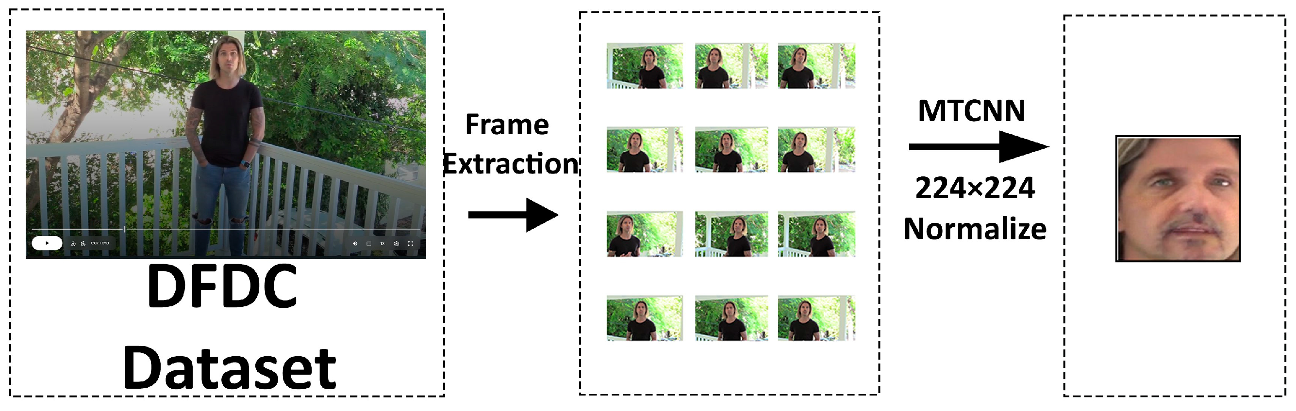
Extracting faces from videos and preparing these faces to meet the model’s requirements form the foundation of the training and evaluation processes. This process is carried out using the extract_faces_from_video function, leveraging tools such as OpenCV and MTCNN. Face detection is performed on each video frame, converting the faces into a format that the model can process and preparing them for training through data transformation processes. The main stages of these operations are illustrated in Figure 2.

In the initial stage, video files are split into frames using OpenCV [21]. The video opened with the cv2.VideoCapture command is processed frame by frame. Face detection on the frames is performed using an MTCNN. The MTCNN detects the position of faces in each frame, marking these faces with rectangular boxes. The coordinates of the faces (x, y, width, height) are identified, these rectangles are cropped, and only the face regions are processed. During this operation, the suppress_stdout function is employed to prevent unnecessary outputs. Images are converted into the PIL.Image format using the Pillow library and prepared for data transformation processes. The progress is displayed to the user using the tqdm library, enhancing the traceability of the process [22].

Data transformation processes are carried out to make the face images suitable for the model’s input. These transformations are defined via the data_transforms object and assembled using the transforms.Compose function. The first transformation, transforms.Resize((224, 224)), resizes all images to 224 × 224 pixels. This resizing is crucial because the model’s input layer expects a specific size, preserving important details in the images while optimizing memory usage. Images are then converted into tensor format using transforms.ToTensor(). The tensor structure provides a three-dimensional representation of RGB color channels, allowing the model to process the data efficiently. Additionally, scaling pixel values to a range between 0 and 1 ensures that the model can adapt to varying lighting and color conditions.

These processes ensure that each video frame’s faces are processed only with the data required by the model, improving the efficiency of the training process. The cropping, scaling, and tensor conversion of faces enable the data to be arranged according to the model’s requirements and eliminate inconsistencies. This structure, created during the training process, allows the model to learn more effectively and produce more accurate results in deep learning applications.

2.5. Definition of Quantum Layers

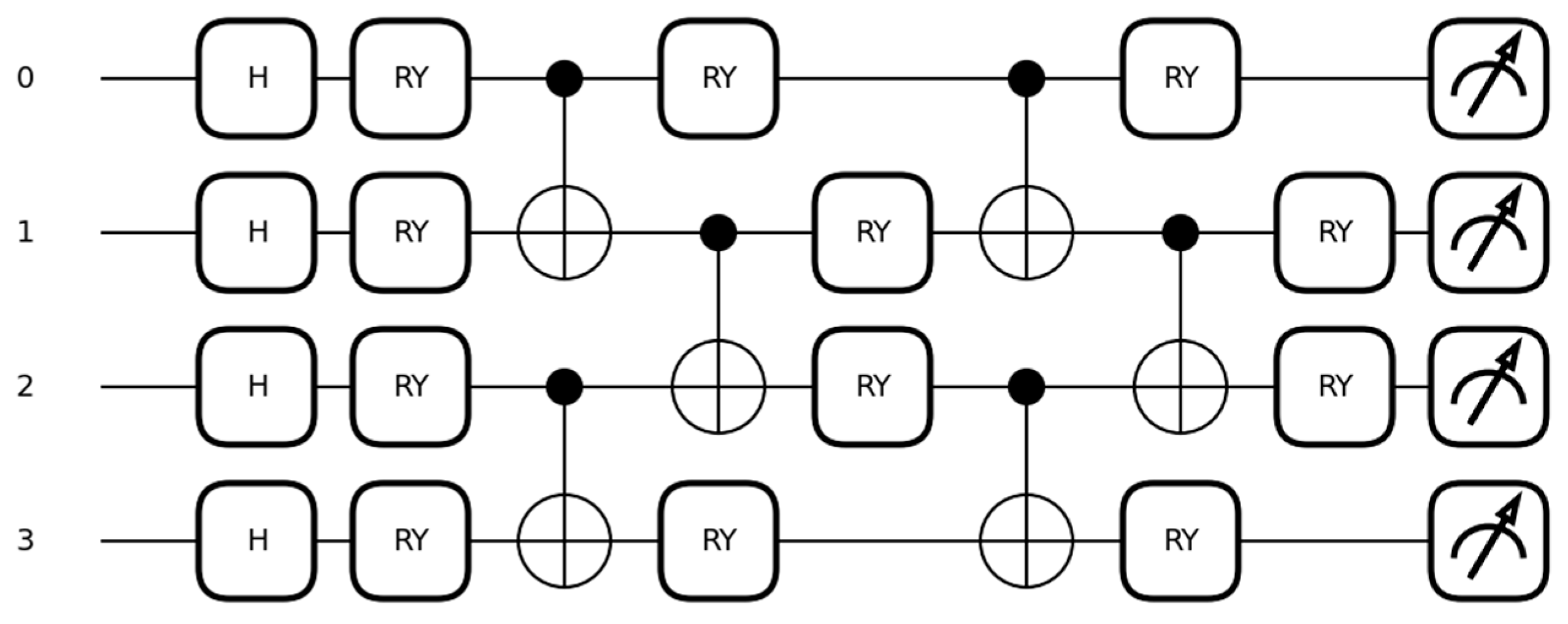
The definition of quantum layers in the model is carried out to perform quantum operations and integrate them with classical learning structures. Quantum layers are defined through functions such as H_layer, RY_layer, and entangling_layer and are used in creating PQCs. These layers calculate data through quantum circuits, integrate quantum information processing features into the model, and offer a perspective distinct from classical learning methods. The model operates by creating superposition, performing parametric transformations, and conducting entanglement processes, all of which collectively expand the model’s learning capacity. Figure 3 visually represents these processes, explaining each stage of the quantum circuit step by step.

The Hadamard gate (H gate) plays a fundamental role in quantum computation by placing qubits into a superposition state, where they simultaneously exist in both |0⟩ and |1⟩ states. This allows quantum systems to process multiple possibilities in parallel, vastly increasing computational efficiency (Nielsen & Chuang, 2010). The RY gate, on the other hand, rotates qubits around the Y-axis of the Bloch sphere based on specific angles, enabling the representation of more complex quantum states and enhancing the model’s ability to analyze diverse data features. Entanglement, achieved through CNOT gates, establishes a quantum correlation between qubits, ensuring that the state of one qubit is dependent on the state of another. This interconnectedness forms the basis for processing complex relationships in quantum systems. Together, these concepts—superposition, rotation, and entanglement—constitute the foundational principles of quantum computation and enable the creation of highly efficient learning models [23].

The computation process begins by applying Hadamard transformations to all quantum bits. This operation places the qubits simultaneously in both |0⟩ and |1⟩ states, creating superposition. Mathematically, this is expressed as follows:

H|0⟩ = 1/√2 (|0⟩ + |1⟩),
    H|1⟩ = 1/√2 (|0⟩ − |1⟩).

(1)

For example, Hadamard gates are applied sequentially to Qubit 0, Qubit 1, Qubit 2, and Qubit 3. Superposition enables parallel computation in quantum information processing, allowing the model to learn more complex data relationships. These transformations are performed on each qubit using the qml.Hadamard(wires = idx) command. This stage of superposition expands the model’s initial knowledge base, providing the fundamental structure needed for subsequent operations [24].

Following the Hadamard transformation, RY transformations are applied using angles derived from the data. Mathematically, the RY gate is represented as follows:

RY(θ)|ψ⟩ = cos(θ/2)|ψ⟩ + sin(θ/2)|ψ⟩.

(2)

This operation rotates the state of each qubit around specified angles, enabling data analysis in various directions. For instance, RY gates are applied to Qubit 0, Qubit 1, Qubit 2, and Qubit 3 sequentially, and these transformations are performed using the qml.RY function. The angles for RY transformations are determined based on data from q_input_features. These angles are optimized during the learning process to adapt to the data, contributing to the model’s ability to evaluate data features from different perspectives. These parametric transformations enhance the model’s flexibility, enabling a deeper learning process [25].

After RY transformations, entanglement operations are performed. At this stage, dependencies between qubits are established using CNOT gates. Mathematically, the CNOT gate operates as follows:

CNOT|ψ⟩ = |ψ⟩ if the control qubit is |0⟩,
    CNOT|ψ⟩ = NOT|ψ⟩ if the control qubit is |1⟩.

(3)

Initially, entanglement is created between Qubit 0 and Qubit 1 and Qubit 2 and Qubit 3, followed by entanglement between Qubit 1 and Qubit 2 in the second stage. This arrangement effectively models relationships among qubits, allowing the model to build a broader network of information. Entanglement operations are executed using the qml.CNOT(wires = [i, i + 1]) command. These operations contribute to the model’s ability to learn more complex data relationships compared to classical systems and strongly represent dependencies among data features [26].

In each quantum depth layer, parametric RY transformations are reapplied, and transformations on each qubit are renewed after entanglement operations. These transformations are carried out using weights determined by q_weights, which are optimized during the learning process to adapt to the model. This stage increases the learning capacity of the model’s quantum circuit and enhances the flexibility of quantum computation operations through parametric transformations. The data learned through these processes are evaluated using measurements based on the Pauli-Z basis, where the measurement operator Z is defined as follows:

Z|0⟩ = |0⟩,
      Z|1⟩ = −|1⟩.

(4)

The measurement results are transferred to classical neural network layers. These measurements are the final outputs of the quantum circuit and directly impact the model’s classification performance [27].

The integration of the quantum circuit with classical learning methods is achieved through the DressedQuantumNet class. This class initiates data processing by converting classical input features into a format compatible with the quantum circuit. Measurement outputs obtained from the quantum circuit are processed through fully connected classical layers, and final classification results are obtained. Parametric weights initialized with random values are optimized during the learning process, contributing to the model’s understanding of the relationship between quantum computation parameters and data. This integration brings quantum and classical information processing methods together, enabling the model to learn more complex data relationships and synthesizing information from both classical and quantum operations. This structure allows the model to leverage the advantages of quantum circuits, expand its data processing capacity, and learn more complex relationships.

2.6. Model Construction

The construction of the model and the arrangement of the final layers were carried out to create a structure that integrates deep learning and quantum layers. This model was built on a pretrained ViT-based architecture. This architecture is based on a transformer structure successfully used in image processing and deep learning tasks, with the capacity to process data with high accuracy. Using the statement timm.create_model(‘cait_s24_224’, pretrained = True), a pretrained ViT model was loaded, and its input features were adapted for image classification tasks.

The ViT operates by dividing an image into fixed-size patches and processing these patches as sequences, similar to words in natural language processing. Mathematically, an input image is divided into patches. Each patch is then linearly embedded into a vector and augmented with positional encodings to retain spatial information. The ViT model processes these embeddings using self-attention mechanisms, computed as follows:

$$\mathrm{A}\mathrm{t}\mathrm{t}\mathrm{e}\mathrm{n}\mathrm{t}\mathrm{i}\mathrm{o}\mathrm{n}\left(\mathrm{Q},\mathrm{K},\mathrm{V}\right)=\mathrm{s}\mathrm{o}\mathrm{f}\mathrm{t}\mathrm{m}\mathrm{a}\mathrm{x}\left({\displaystyle \frac{\mathrm{Q}{\mathrm{K}}^{\mathrm{T}}}{\sqrt{{\mathrm{d}}_{\mathrm{K}}}}}\right)V$$

(5)

where $\mathrm{Q}$, K, and V are the query, key, and value matrices derived from the input embeddings, and ${\mathrm{d}}_{\mathrm{K}}$ is the dimensionality of the key vectors. This mechanism allows the model to focus on different parts of the image to learn complex patterns [28].

The CaiT (Class-Attention in Image Transformers) model is an extension of the ViT, designed to improve the convergence and performance of transformers in image classification tasks. The CaiT introduces class-attention layers that separately process the class token, enabling the model to focus specifically on classification-related features. This is mathematically represented as follows:

$$ClassAttention\left({\mathrm{Q}}_{\mathrm{c}},\mathrm{K},\mathrm{V}\right)=\mathrm{s}\mathrm{o}\mathrm{f}\mathrm{t}\mathrm{m}\mathrm{a}\mathrm{x}\left({\displaystyle \frac{{\mathrm{Q}}_{\mathrm{c}}{\mathrm{K}}^{\mathrm{T}}}{\sqrt{{\mathrm{d}}_{\mathrm{K}}}}}\right)V$$

(6)

where ${\mathrm{Q}}_{\mathrm{c}}$ is the class token query and $\mathrm{K}$ and $\mathrm{V}$ are the key and value matrices from the patch embeddings. These additional layers allow the CaiT to refine the class-specific representations and achieve higher accuracy on image classification benchmarks [29].

The output features of the deep learning structure were adjusted in a multi-layer fully connected layer sequence to suit the DressedQuantumNet class. During this arrangement, fully connected layers of various dimensions were added sequentially and supported with ReLU activation functions. In this layer structure, the 1000-dimensional feature vector from the deep learning model was reduced to dimensions of 512, 256, 128, and 64, respectively. This process preserves the overall structure of the model while extracting smaller, meaningful features. After these stages, the data are transferred to the DressedQuantumNet class and processed with quantum operations.

In the model, the final layers of the loaded Vision Transformer architecture were replaced with the DressedQuantumNet class. This class was designed to integrate quantum computing layers with classical deep learning layers to process data in a more complex structure. Replacing the final layers of the model was carried out with the aim of creating a new classifier suitable for its task.

After the final layer adjustments, the model was loaded onto a CUDA or CPU device as appropriate. During the model construction phase, path parameters were defined for directories where the final model would be saved and for paths to save the intermediate outputs of the model. This configuration allows the model to retain its state after each step in the training process and continue from where it left off when needed. With the final layer adjustments, the Vision Transformer-based model was made capable of analyzing data within multidimensional relationships through the combination of classical and quantum layers.

As shown in Figure 4, this structure enables the model to undergo a learning process that integrates quantum and classical deep learning layers, allowing the model to make deeper and more versatile inferences from the data. This enhances the model’s capacity for information processing and offers an effective structure for multidimensional data analysis.

2.7. Model Training Process and Optimization Settings

The model training process and optimization settings were carefully structured to achieve the best performance and minimize error rates during the training phase. The training process was supported by optimization algorithms and loss functions that update model parameters throughout the learning process. The Adam optimization algorithm and cross-entropy loss function were used in training, aiming for high accuracy and low error rates in the classification task.

Throughout the training process, model outputs, accuracy rates, and loss values were periodically monitored, and optimization parameters were updated when necessary. The optimization settings and loss function employed during training enabled the model to learn effectively, ensuring that it functioned as a highly accurate and generalizable classifier after training.

2.8. Loading the Dataset and Extracting Labels

The process of loading the dataset and extracting labels is one of the essential data preparation steps required for proper model training. In this process, the videos and their labels in the dataset are prepared for the training phase. The DFDC dataset, which includes a large collection of fake (FAKE) and real (REAL) videos, was utilized.

The dataset loading process begins with reading the metadata.json file. This file contains the labels for each video in the dataset, providing a “FAKE” or “REAL” label for every video. Located in the main folder defined as input_path, this file enables the model to identify whether a video is fake or real during loading. In the code, the command with open(os.path.join(input_path, “metadata.json”), ‘r’) as f opens this file and transfers all labels into the all_metadata variable. This setup allows the model to easily access the label of each video file.

The separation of videos based on their labels is a process that classifies them as fake (FAKE) or real (REAL). Using the information in the metadata file, videos labeled as fake are added to one list, while videos labeled as real are added to another. This process enables the model to correctly differentiate between fake and real videos during training, contributing to a balanced training process. This separation ensures that the model learns equally from both types of videos during training.

To maintain a balanced training process, fake and real videos are periodically moved to the output_path directory during training. Through this operation, processed videos are organized for reuse during the training process, and after each video is processed, the metadata.json file is updated to keep track of processed videos. This process ensures that the training process progresses systematically by recording which videos the model has processed at each step.

These loading and label extraction processes enable the model to efficiently use the videos in the dataset, allowing it to accurately distinguish between fake and real data. The balanced use of the dataset during training and the proper processing of data with accurate labels contribute to the model’s effective learning process and its ability to achieve high accuracy in the deepfake detection task.

2.9. Processing Fake and Real Videos During Training

The video processing phase continues with the model’s training and optimization steps. Each face frame is transferred to the model’s input layer and classified as fake or real by the model. The labels predicted by the model are compared with the actual labels, and an error value is calculated using the cross-entropy loss function. This error value is minimized using the Adam optimization algorithm through backpropagation to improve the model’s learning process by updating its parameters.

During training, the model’s performance is measured using metrics such as accuracy and loss. At the end of each training step, the accuracy value is calculated by comparing the number of correctly classified frames with the total number of frames. During this process, the model’s predictions are compared with the actual labels, and metrics such as the accuracy rate, the loss value, and other classification performance indicators are recorded for each video.

In the later stages of training, when the remaining number of fake and real videos reaches a certain level, metrics such as loss and accuracy are analyzed in detail. At the end of the training process, classification reports and confusion matrices are calculated to evaluate the model’s performance. In particular, the number of correctly predicted fake and real frames, overall accuracy rate, and misclassification counts are reviewed.

Finally, each processed video is moved to the designated output_path directory, allowing the next video to be processed for training. During the training process, the processing status of videos is updated in the metadata.json file, recording which videos the model has processed and ensuring that the training process progresses systematically. These steps enhance the model’s ability to distinguish between fake and real videos, contributing to high accuracy and performance in the deepfake detection task.

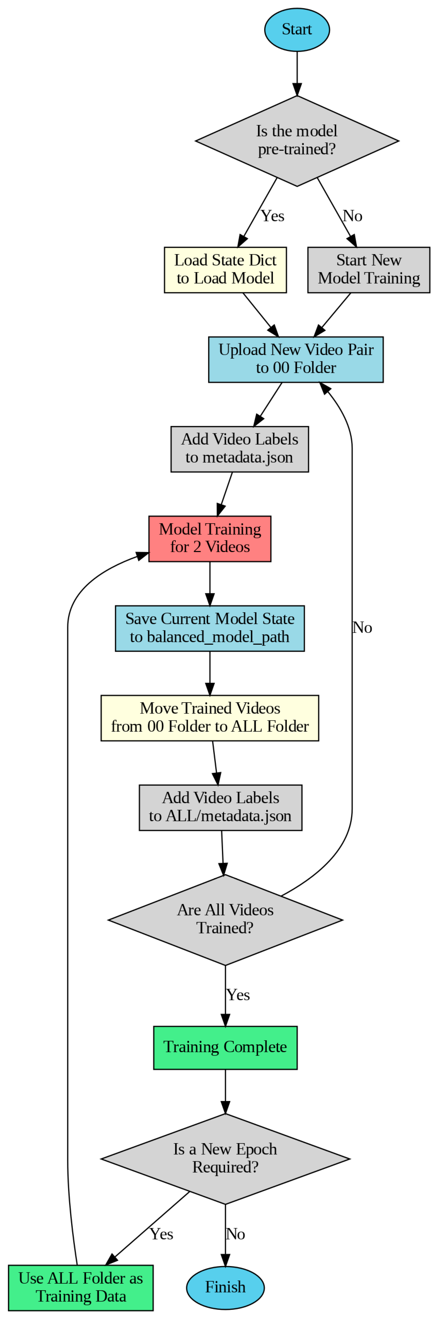
2.10. Training Process Tracking and Model Continuity

In this study, a customized model training strategy was adopted to efficiently process the large dataset used in the deepfake detection task within the limited session duration of Google Colab. Since the session duration on the Google Colab platform is generally limited to 24 h, a specific saving mechanism was developed to ensure that the model could resume training from where it left off in each session. This mechanism involves recording the current state of the model and tracking the training data step by step.

The dataset used consists of the DFDC (Deepfake Detection Challenge) dataset divided into 50 different parts, containing a total of 124,000 videos. To prevent the model from focusing solely on fake data, as most of the dataset is labeled FAKE, and to ensure balanced learning, the videos in each part were grouped as one FAKE and one REAL video. As a result of this limitation, the model was trained using a total of 25,000 videos.

During the training process, the current state of the model was saved to the balanced_model_path after every two videos, ensuring that the most recent state of the model was preserved so that it could continue from where it left off in the next session. In this structure, two main folders were defined: the 00 folder, where the current data parts from the DFDC dataset are loaded during processing, and the ALL folder, where trained video data are stored. After every two-video training cycle, the training data in the 00 folder are transferred to the ALL folder to avoid repetition in training. This ensures that when a session ends and a new session begins, the model continues training only with videos that were not processed in the previous session.

At this stage, metadata.json files were used to track the data labels used in training. The metadata.json file in the 00 folder holds the labels of the videos to be processed in the current part, while the metadata.json file in the ALL folder accumulates the labels of the processed videos. In case the training process is interrupted for any reason, the model resumes from where it left off by loading the model state from the balanced_model_path using the load_state_dict command. This approach ensures that all videos are included in the training process and prevents redundant processing, achieving high efficiency. Additionally, collecting the processed videos in the ALL folder allows them to be directly used as training data if multiple epochs are desired.

As shown in Figure 5, this structure enables efficient training of the model under limitations such as a restricted session duration and a large dataset.

3. Results

To evaluate the performance of the model during the training process and measure its ability to distinguish between fake (FAKE) and real (REAL) videos, various metrics were calculated. This process provides a broad evaluation spectrum, ranging from basic measures such as accuracy, precision, recall, and F1 and F2 scores to more complex performance analyses like the Matthews Correlation Coefficient (MCC) and ROC AUC. At the end of training, the overall success of the model was analyzed using tools such as classification reports, confusion matrices, and ROC curves. These analyses play a critical role in assessing the model’s potential for real-world applications in deepfake detection.

The classification metrics used to evaluate the model’s performance are summarized in

Table 1. Classification metrics formulas and their descriptions.

Metric	Formula	Description
Precision	TP/(TP + FP)	TP (True Positive): correctly predicted positive instances. FP (False Positive): incorrectly predicted positive instances among negatives.
Recall	TP/(TP + FN)	TP (True Positive): correctly predicted positive instances. FN (False Negative): positive instances incorrectly predicted as negative.
F1 Score	$2\times {\displaystyle \frac{\mathrm{P}\mathrm{r}\mathrm{e}\mathrm{c}\mathrm{i}\mathrm{s}\mathrm{i}\mathrm{o}\mathrm{n}\times \mathrm{R}\mathrm{e}\mathrm{c}\mathrm{a}\mathrm{l}\mathrm{l}}{\mathrm{P}\mathrm{r}\mathrm{e}\mathrm{c}\mathrm{i}\mathrm{s}\mathrm{i}\mathrm{o}\mathrm{n}+\mathrm{R}\mathrm{e}\mathrm{c}\mathrm{a}\mathrm{l}\mathrm{l}}}$	Combines precision and recall into a single metric. Balances the trade-off between false positives (FPs) and false negatives (FNs).
Accuracy	${\displaystyle \frac{\mathrm{T}\mathrm{P}+\mathrm{T}\mathrm{N}}{\mathrm{T}\mathrm{o}\mathrm{t}\mathrm{a}\mathrm{l} \mathrm{N}\mathrm{u}\mathrm{m}\mathrm{b}\mathrm{e}\mathrm{r} \mathrm{o}\mathrm{f} \mathrm{I}\mathrm{n}\mathrm{s}\mathrm{t}\mathrm{a}\mathrm{n}\mathrm{c}\mathrm{e}\mathrm{s}}}$	TP (True Positive): correctly predicted positives. TN (True Negative): correctly predicted negatives. Represents overall classification success.
ROC AUC	${\displaystyle \sum _{i=1}^{n-1}}{\displaystyle \frac{\left(x_{i+1}-x_i\right)\cdot \left(y_i+y_{i+1}\right)}{2}}$	$x_i$ (FPR): False Positive Rate. yi (TPR): True Positive Rate. n: total thresholds.

. These metrics—precision, recall, F1 score, accuracy, and ROC AUC—offer a comprehensive framework for assessing the model’s ability to classify fake and real videos. Precision evaluates the proportion of correctly identified positive predictions among all positive predictions, providing insight into the model’s accuracy in predicting the positive class [30]. Recall, also known as sensitivity, measures the proportion of actual positive instances correctly classified [30]. The F1 score balances precision and recall by considering both false positives and false negatives, offering a single metric that reflects the model’s overall effectiveness in positive classification tasks [31]. Accuracy calculates the proportion of correctly classified instances, including both positive and negative examples, across the entire dataset [32]. Finally, the ROC AUC quantifies the model’s ability to differentiate between classes by calculating the area under the Receiver Operating Characteristic curve, which is constructed based on False Positive Rate (FPR) and True Positive Rate (TPR) values across various thresholds [33]. The descriptions in the table provide detailed explanations of the parameters used in these calculations, ensuring clarity and interpretability for readers.

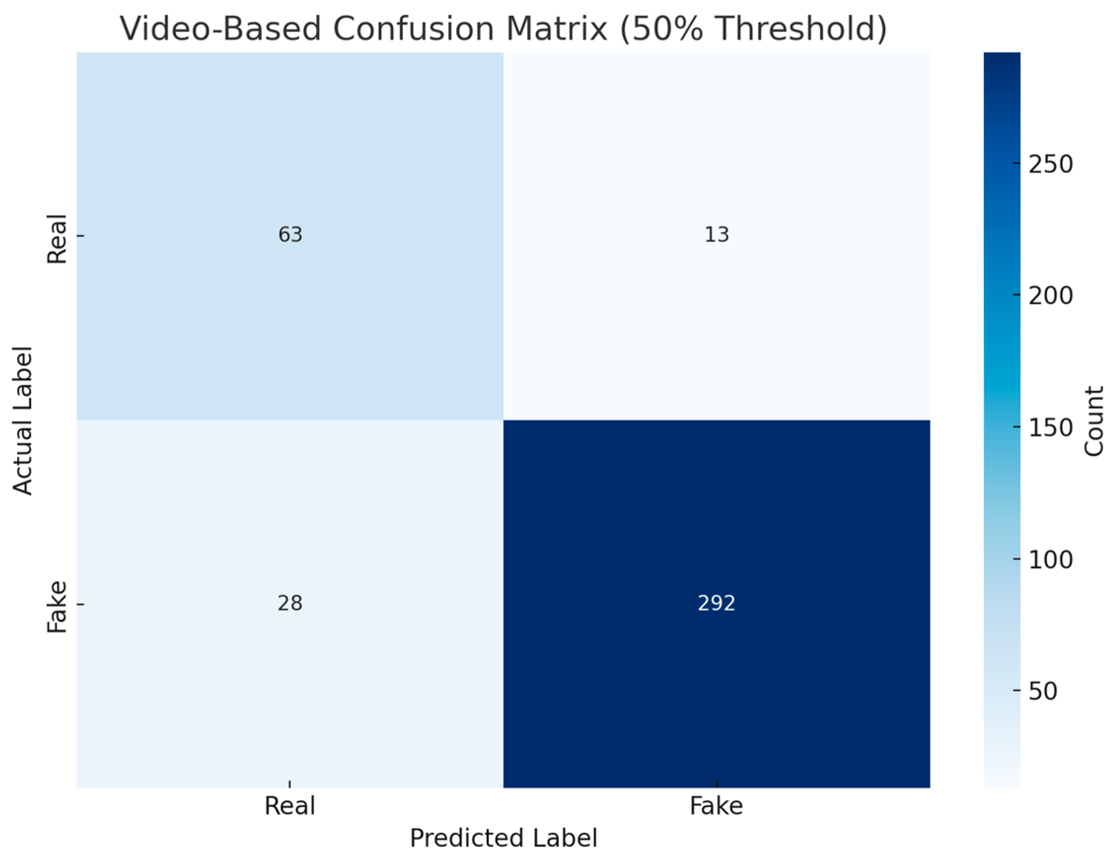
To visualize the model’s performance, the confusion matrix shown in Figure 6 categorizes the model’s correct and incorrect classifications into four main categories. For real videos, the number of correct classifications was 63, while the number of incorrect classifications was 13. Similarly, for fake videos, the number of correct classifications was 292, and the number of incorrect classifications was 28. The confusion matrix reveals that the model exhibits a very high success rate in distinguishing fake videos. However, its relatively lower performance in real videos indicates the need for optimization in this data type.

The ROC curve in Figure 7 was used to evaluate the classification performance of the model. The area under the ROC curve (AUC) was calculated as 0.94, indicating that the model possesses a high discriminatory power. The curve illustrates the relationship between the False Positive Rate (FPR) and the True Positive Rate (TPR) across all threshold values. These results emphasize the model’s strong performance, particularly in accurately classifying fake content.

The details presented in

Table 2. Classification metrics showing the model’s class-based performance.

Metric	Precision	Recall	F1 Score	Support
Real	0.69	0.83	0.75	76
Fake	0.96	0.91	0.93	320
Accuracy			0.90	396
Macro-Avg.	0.82	0.87	0.84	396
Weighted Avg.	0.91	0.90	0.90	396

provide an opportunity to evaluate the model’s performance for each class separately. For the real class, the precision was determined as 0.69, the recall as 0.83, and the F1 score as 0.75. For the fake class, these values were measured as 0.96, 0.91, and 0.93, respectively. The overall accuracy of the model was calculated as 90%. This indicates that the model demonstrates strong performance, particularly in detecting fake videos, but requires further optimization for the classification of real videos.

To summarize the overall performance of the model, weighted average values were used, as given in

Table 3. Key metrics calculated for classification performance.

Metric	Precision	Recall	F1 Score	ROC AUC
Value	0.91	0.90	0.90	0.94

. This approach was chosen due to the imbalance in the test dataset, where the “fake” class contains more data. The model’s precision was calculated as 0.91, the recall as 0.90, and the F1 score as 0.90, while the ROC AUC score was determined to be 0.94. These metrics indicate that the model demonstrates consistent performance across both classes and achieves successful classification at all threshold levels. The use of weighted average values minimizes the impact of dataset imbalance and provides a more realistic reflection of the model’s overall performance. However, while these results confirm the model’s superior performance in the “fake” class, they also highlight the need for improvement in the “real” class. Evaluating the data in this manner ensures a more reliable assessment of the model’s classification success in real-world scenarios.

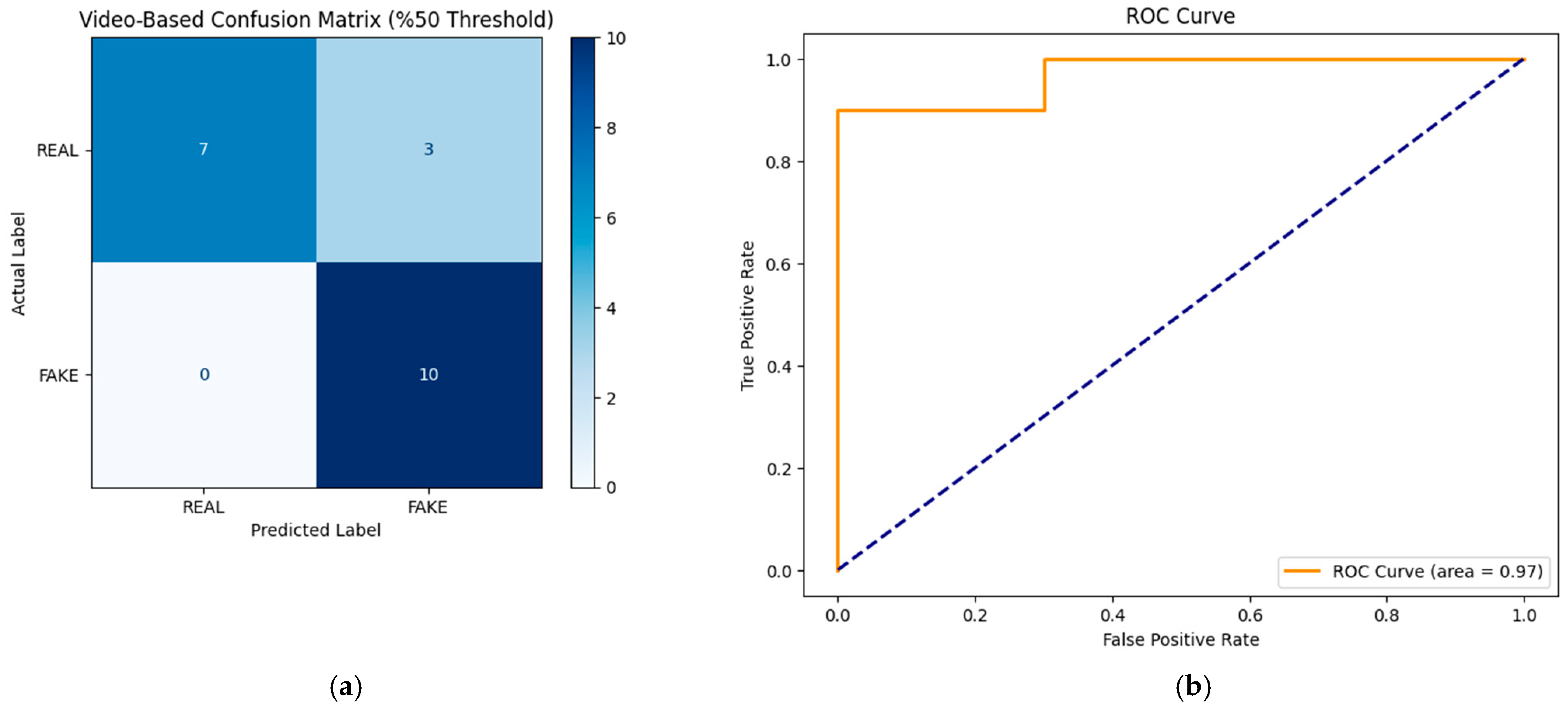
To evaluate the generalizability of the model across datasets, a cross-dataset test was performed using a subset of the CelebDF-v2 dataset [34]. The evaluation included 10 real and 10 fake videos, selected to provide an initial assessment of the model’s performance on unseen data. The results of this evaluation are summarized in

Table 4. Classification metrics showing the model’s class-based performance on the cross-dataset evaluation.

Metric	Precision	Recall	F1 Score	Support
Real	1.00	0.70	0.82	10
Fake	0.96	0.91	0.93	10
Overall	0.88	0.85	0.85	20

, and the corresponding visualizations are provided in Figure 8.

The classification performance metrics, including precision, recall, and F1 score, indicate that the model achieved an overall accuracy of 85% with a macro-average F1 score of 0.85. The ROC curve further highlights the model’s classification capability, with an AUC score of 0.97, demonstrating robust performance on previously unseen data. The detailed metrics are presented in Table 4, reflecting the model’s ability to distinguish between videos labeled REAL and FAKE effectively.

These results provide an initial indication of the model’s generalizability to other datasets and suggest its applicability in diverse deepfake detection scenarios.

All these metrics highlight both the strengths and areas for improvement of the model. The loss values calculated during training and the model’s performance progression were analyzed, showing that the model improved its learning capacity over time. However, the low precision and recall rates achieved for the real class indicate the need to diversify the dataset and optimize the training duration. In light of these analyses, improvements such as collecting additional data, optimizing the model architecture, and training with a larger dataset are recommended to enhance the model’s performance. This approach will strengthen the model’s ability to more accurately distinguish between fake and real videos.

4. Discussion

In this study, a model was developed for deepfake detection using a combination of the QTL and ViT architectures. The primary aim of the study was to overcome the limitations of existing methods by proposing a system that ensures both computational efficiency and high accuracy rates. Although the QTL and ViT architectures have been used in various fields, no prior study has combined these two technologies for deepfake detection. The proposed method aims to provide a more generalized solution capable of detecting spatial and temporal inconsistencies by merging these innovative technologies.

The results obtained indicate significant success in deepfake detection. With a 90% accuracy rate, the model demonstrated substantial performance improvements compared to other studies based on previous research.

Table 5. Comparative analysis of deepfake detection studies on the DFDC dataset.

Subject	Methods	DFDC Accuracy	DFDC ROC AUC
Quantum Transfer Learning and Class-Attention Vision Transformer Architecture (This Study)	QTL and CaiT	90%	0.94
Towards More General Video-based Deepfake Detection through Facial Feature Guided Adaptation for Foundation Model [6]	CLIP	Unspecified	0.909
Deepfake Detection with Deep Learning: Convolutional Neural Networks versus Transformers [10]	ResNet, Swin Transformer	92.02%	0.9761
A Hybrid CNN-LSTM model for Video Deepfake Detection by Leveraging Optical Flow Features [11]	CNN-LSTM	66.26%	Unspecified
Deepfake Video Detection Using Convolutional Vision Transformer [12]	Convolutional Vision Transformer	91.5%	0.91
Deepfake Detection by Analyzing Convolutional Traces [7]	Convolutional Traces	87%	Unspecified
Deepfake Detection Using Multi-Attentional Techniques [8]	Multi-attention Mechanisms	89.5%	0.92
Joint Audio-Visual Deepfake Detection [9]	ResNet, Swin Transformer	92.1%	Unspecified

presents a comparative analysis of the proposed model with other prominent works in the literature. For instance, the study “Deepfake Detection with Deep Learning: Convolutional Neural Networks versus Transformers” reported 92.02% accuracy and a 97.61 AUC. Similarly, the study “Towards More General Video-based Deepfake Detection through Facial Feature Guided Adaptation for Foundation Model” achieved strong performance in cross-dataset adaptability, with a 90.9 AUROC on the DFDC dataset. However, considering the high hardware requirements and resource demands of these models, their applicability in real-world scenarios remains limited.

5. Conclusions

The originality of this model stands out not only due to the results obtained but also because of the innovative methodology employed. The advantages of quantum computing provided by QTL were combined with the global feature extraction capacity of the CaiT, enabling the detection of subtle details in deepfake videos. In particular, the CaiT’s ability to detect small-scale forgery details in visual data is considered one of the model’s strongest aspects. Additionally, the benefits offered by QTL facilitated a more efficient learning process on large datasets, accelerating the training process and increasing the model’s generalization capacity.

Despite its strengths, this study also has some limitations. The model was tested only in a simulated quantum environment, and no evaluation was conducted on a real quantum device. This partially limits the generalizability of the results. Furthermore, the DFDC dataset is one of the largest and most diverse datasets used for deepfake detection. However, due to hardware and time constraints, only 50% of the dataset was utilized in this study. For instance, CNN-LSTM-based models in the literature achieved 98.2% accuracy using the full dataset. Utilizing the entire dataset could provide a more comprehensive evaluation of the model’s performance and potentially improve its accuracy.

A comparative analysis of the proposed QTL-CaiT model against state-of-the-art deepfake detection methods is presented in

Table 6. Comparative analysis of deepfake detection studies using Vision Transformer-based and hybrid models.

Subject	Methods	Dataset	Accuracy
Quantum Transfer Learning and Class-Attention Vision Transformer Architecture (This Study)	QTL and CaiT	DFDC	90%
Efficient Deepfake Detection Using Vision Transformers [35]	CViT	DFDC	85%
Improved Deepfake Video Detection Using Convolutional Vision Transformer [36]	CViT2	DFDC	95%
FakeFormer: Vulnerability-Driven Transformers for Deepfake Detection [37]	FakeFormer	DFDC (cross)	78.91%
Feature Fusion Vision Transformers for Deepfake Detection [38]	ViT + MLP-Mixer	DFDC (cross)	52.95%
Hybrid Vision Transformer for Deepfake Detection [39]	CAEs + ViT	OpenForensics	87%

. The table highlights the performance of various models, including transformer-based architectures and hybrid approaches, evaluated on different datasets. Notably, the QTL-CaiT model achieves a high accuracy of 90% on the DFDC dataset, showcasing its competitive edge in performance. Compared to other methods, such as CViT and FakeFormer, the proposed model demonstrates both robustness and effectiveness in handling deepfake detection tasks, further emphasizing its potential applicability in diverse scenarios.

The proposed QTL-CaiT model demonstrates a total parameter count of approximately 24.7 million, which includes 24 million parameters from the Vision Transformer (CaiT), 686,992 parameters from the fully connected layers, and 86 parameters from the Quantum Neural Network (QNN). During the training process, the total RAM usage was observed to be approximately 12–13 GB. This memory consumption accounts for the storage of model parameters (~98.74 MB), intermediate activations generated during forward and backward passes, optimizer states, and batch data loaded into memory. Each batch, with a size of 32 and input dimensions of 224 × 224 pixels, occupied approximately 192 MB of memory. The Vision Transformer component required an estimated 10–20 GFLOPs due to its computational complexity, while the fully connected layers added approximately 21.89 MFLOPs. The QNN contributed minimally to computational overhead, emphasizing the model’s lightweight and efficient design. Additionally, the average processing time per video was approximately 4 min, making it computationally intensive for large datasets. Together, these components underline the model’s efficient use of computational resources, balancing complexity and performance while maintaining robust results in deepfake detection tasks.

The main challenges in deepfake detection are the diversity of fake videos and the continuously evolving forgery techniques used to produce them. The proposed method has the potential to address existing gaps in the literature. However, future studies should focus on adapting the model for real-time applications and improving its applicability on low-resource devices. Moreover, testing the model on larger and more diverse datasets could contribute to enhancing its overall performance.

In conclusion, this study presents a novel approach to deepfake detection by combining the CaiT and QTL. Unlike existing studies in the literature, it has optimized resource efficiency while introducing a new perspective to deepfake detection. The findings provide a foundation for broader-scale research and applications. This method could guide the development of new models aimed at detecting more sophisticated forgery techniques in the future.

Future studies could focus on testing the model on real quantum devices and training it on larger, more diversified datasets. Additionally, optimizing the model for real-time forgery detection, making it usable on low-resource devices, and integrating multimodal (e.g., visual, audio) analyses could open new horizons in the field of deepfake detection. Furthermore, testing the model’s robustness against malicious techniques, such as intentional manipulations or deceptive inputs, and improving its security level could be important steps for future research.