Abstract
Curve squeal is a highly disturbing tonal noise produced by railway vehicles on tight curves, primarily attributed to lateral sliding at the wheel–rail interface. An essential step to estimate curve squeal noise levels is to determine the nonlinear self-sustained vibrations, for which time integration is a commonly used method. However, although it is known that the initial conditions affect the solutions obtained with time integration, their impact on the limit cycles is often overlooked. This study investigates this aspect for a curve squeal model based on falling friction and a modal reduction of the wheel and provides some insights on the mode competition phenomena and the nature of the final limit cycles obtained. The paper first details the curve squeal model, stability analysis, as well as the initial condition derivation, and then discusses the time integration and limit cycle results in both time and frequency domains. The results reveal two primary families of limit cycles that can be obtained for both types of initial conditions. The cases where stationary vibrations result in a quasi-periodic regime converge to a unique limit cycle which displays three fundamental frequencies corresponding to specific wheel modes, plus harmonic interactions among them.
1. Introduction
Curve squeal is a highly disturbing type of railway noise that occurs when the vehicle is in motion at tight curves under certain operation and environmental conditions. It is characterized by a high-pitched intense and tonal sound, with sound energy being concentrated at pure frequencies, typically beyond 500 Hz. The relative lateral velocity between the wheel and the rail, induced by a high angle of attack due to an imperfect curving behavior, is widely accepted as the main cause of curve squeal and it is commonly explained by two potentially coexisting mechanisms: instabilities due to falling friction and geometrical instabilities at constant friction [1].
Falling friction was first introduced by Rudd [2] in the 1970s and has been used since as the basis for other more detailed curve squeal models [3,4,5,6]. It suggests that a decreasing friction coefficient at the wheel–rail interface with respect to lateral sliding velocity acts as an equivalent negative damping that feeds energy into the system, leading eventually to self-sustained vibrations and hence curve squeal. As explained by Chiello [6], three phases may be distinguished in the time domain vibrations: first, the wheel slides with respect to the rail and, due to falling friction, the equivalent damping is negative, so that the lateral velocity starts to grow at a rate governed by the modal growth rates until the saturation velocity is reached. In the second phase, the wheel contact point begins to creep, as the nonlinearities of the friction force slow down the amplitude growth (the equivalent damping is positive in some phases of the oscillation); the unstable modes are in competition until one or some of them become dominant. Finally, the lateral velocity stabilizes and the solution converges to a stationary regime, or limit cycle. On the other hand, the geometrical instabilities mechanism, introduced later, suggests that, unlike on falling friction, instabilities can still occur at a constant friction coefficient, thanks to the coupling between the tangential and the normal dynamics [7,8,9,10,11,12,13], where the rail may play an important role. As Hoffmann [7] explained, the normal force fluctuations influence the lateral force, but not vice versa, leading to an asymmetric stiffness matrix, which can induce mode-coupling instabilities. Moreover, Ding et al. [10], as well as Jiang et al. [12] showed that single wheel modes can couple with the rail and produce squeal, in a way that is somewhat different than the mode coupling phenomenon, due to the large apparent damping provided by the rail at the contact point.
In squeal models, the occurrence of the phenomenon is often determined by a stability analysis. One commonly used method which is well adapted to a modal description of the structures is the analysis of the complex eigenvalues of the system [6]. Other methods exist, however, in which the structures are described in the frequency domain via their mobilities and the Nyquist’s criterion is used to determine the unstable frequencies of the system [5]. Stability analysis involves the linearization of the contact forces and, therefore, it can only be regarded as a first step into the study of curve squeal, as it cannot determine the vibration levels and excitation frequency of a system subjected to self-sustained vibrations; determination of the nonlinear self-sustained vibrations is then required. Two families of methods can be used: those based on the integration (typically numerical) of the dynamic equations of the system in the time domain [6,10,14,15] and those involving a direct limit cycle search in the time or in the frequency domain, such as the shooting method [16] and the Constrained Harmonic Balance Method [17].
Furthermore, time integration methods (for curve squeal models), can be subdivided into those based on the condensation of the wheel and rail behavior at their contact degrees of freedom [9,18], which involve computing impulse responses and solving integral-differential equations, and those based on spatial discretization of the vibration fields of the structures (mostly of modal type) [6,19], which translates into solving second-order systems of differential equations.
It is clear that the solution obtained with time integration methods (irrespective of their classification) depends on the initial conditions used. In spite of this, their choice is not generally discussed or is partially justified, mostly because the implicit but inaccurate hypothesis that the final limit cycle is independent of the initial conditions is accepted. However, previous works in the wider field of friction-induced vibrations have pointed out the existence of different limit cycles depending on the initial conditions. For example, Loyer et al. [20] were able to obtain different limit cycles for a simple sliding elastic layer and these limit cycles could be of periodic or quasi-periodic nature and have different fundamental frequencies, depending on the parameters of the model, the total number of unstable modes, and also the initial conditions used. For curve squeal in particular, Chiello [6] demonstrated that by favoring a particular mode in the initial conditions, by imposing a non-zero modal contribution to it, led to a different limit cycle than would be obtained with similar modal contributions for all unstable modes. The influence of harmonically-related modes on the frequencies that appeared in the final limit cycle was also highlighted in this study, where there is a factor of 2 between the natural frequencies of two specific wheel modes. Lai et al. [21] also stated that initial conditions act on the limit cycle and dominant frequencies, although no further details were given.
The types of initial conditions generally used on curve squeal models are a zero initial position at rest [22,23], the quasi-static equilibrium [8], a static disturbance of the equilibrium [24], a non-zero relative velocity and initial position at equilibrium [6], and a progressive application of creepage and normal load [9]. These conditions are expressed in terms of physical quantities such as velocity or position, which means that they could be directly linked to the operating conditions, such as surface irregularities or the variation of the angle of attack during the curve. However, for time integration using a modal description of the structures, initial conditions in terms of the modal contributions need to be imposed, as performed by Loyer et al. [20], but these initial conditions do not have a physical meaning per se, which limits their comprehension.
Finally, in terms of noise levels, it is well established that squeal noise is primarily radiated by the wheel in axial vibrations [1]. Moreover, the spectrum of radiated noise is very close to the spectrum of self-sustained vibrations, since the sound radiation factors of the vibration modes involved in curve squeal are very close to each other. The calculation of these radiation factors is well controlled and can be carried out in the same way as for the prediction of rolling noise, using for instance numerical techniques such as Boundary Element Methods [21] or approximate analytical formulae [25]. Consequently, the main issue is the determination of the self-sustained vibrations.
The objective of this article is thus to assess the impact of initial conditions on the final limit cycle obtained with numerical time integration for a curve squeal model based on the falling friction mechanism and using a modal description of the wheel. Although the track and the vertical dynamics may have a significant influence on the system vibration (as mentioned above), the model used in this study neglects the track and considers only the lateral friction for two reasons: firstly, the inclusion of the track is not necessary to capture the essence of the falling friction mechanism and, secondly, representing the behavior of the track in modal terms (so that time integration based on spatial discretization of the vibration fields can be performed) is inaccurate or, at least, would lead to unnecessary complications, such as the necessity of a pseudo-modal approach [19,26]. These complications are beyond the scope of this article. A consequence of this assumption is also that the effect of wheel–rail roughness on the self-sustained vibrations is neglected. Two types of initial conditions are studied, the modal-derived and the physically-derived ones, and for the latter a formulation allowing to relate the physical quantities to the modal quantities is described.
The article is structured in two parts. First, the curve squeal model used is detailed, with its corresponding governing equations of motion, friction model and main parameters; the equations of the stability analysis of the system, as well as the derivation of the initial conditions constituting the test cases of this study, are then presented. Secondly, the results are discussed, providing an analysis of the limit cycles obtained in the time domain and in the frequency domain and paying special attention to the mode competition phenomena.
2. Materials and Methods
2.1. Description of the Model
For the wheel–rail interaction model, we consider the inner wheel of the leading bogie of a vehicle in a right curve (cf. Figure 1). For right curves, the angle of attack between the wheel and the rail’s tangent is always positive in the coordinate system shown in Figure 2 for the internal wheels, which are of major interest for curve squeal.
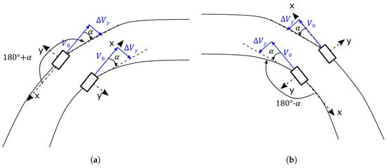
Figure 1.
Coordinate system on right (a) and left (b) curves.
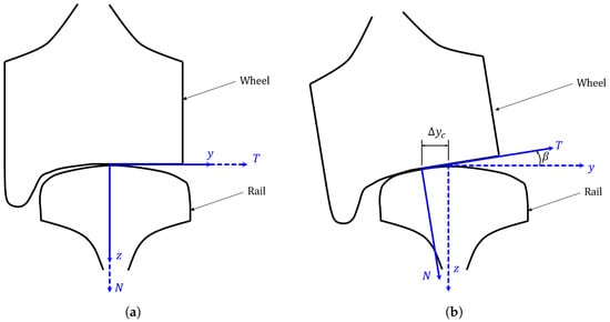
Figure 2.
Coordinate system of the model, nominal (a) and shifted (b) configurations.
The contact at the wheel–rail interface is considered point-like, with a Eulerian reference frame attached to the nominal contact point as shown in Figure 2. The x-coordinate points along the rolling direction of the vehicle, the y-coordinate is the lateral direction pointing inwards to the curve and the z or vertical direction points downward into the rail. A lateral offset with respect to the nominal contact point, , as well as the contact plane angle , is taken into account in the model. These two parameters are assumed to be constant during the curving behavior and a coordinate transformation is required to pass from the nominal reference frame to the shifted reference frame.
The model comprises only one degree of freedom condensed at the wheel–rail contact point and the wheel’s modal base is calculated by finite elements using commercial software. The track is considered infinitely rigid in the lateral direction, which is marked “T” in Figure 2. The normal dynamics are not taken into account in the model, as the fluctuations of the normal force caused by the track are neglected and the vibrations are assumed to occur only along the lateral direction. Because of this, the terms “lateral” and “tangential” will be used interchangeably from now on and notation u and v, for instance, will refer to the displacement and the velocity at the contact point and in the lateral direction.
2.1.1. Contact Forces
Since the normal dynamics are neglected, the normal contact force corresponds only to the constant static load N of the vehicle’s weight on one wheel. Tangential forces, on the contrary, which are characterized by rolling friction theory [27], increase linearly with respect to the relative sliding velocity at small creepages (creepage s is the sliding velocity normalized by the rolling velocity), due to the deformation of the interface during rolling [6]; at higher creepages, however, a saturated regime is reached, where the equivalent friction coefficient is equal to the Coulomb coefficient .
The lateral creepage contains a quasi-static component that is approximately equal to the angle of attack and a dynamic component that depends on the wheel’s vibrations. It is defined as:
Shen–Hedrick–Elkins’ friction/creep law [28] is used to model the nonlinear frictional forces at the wheel–rail interface [25]. Furthermore, in the saturated regime, a decaying friction coefficient with respect to creepage s is described by a function of the form , where is the parameter that governs the decay rate [14]. This feature is what the falling friction model mentioned in the introduction suggests is the cause of the instabilities associated with the curve squeal phenomenon.
2.1.2. Equations of Motion
The system of equations that govern the wheel is directly presented in modal coordinates, where the modal base is calculated by finite elements, with n modes and one physical degree of freedom corresponding to the contact point [6], as follows:
are the generalized mass, damping and stiffness matrices of the wheel, respectively, and proportional damping is assumed, so that matrix is diagonal. stands for the creepage and normal force-dependent friction coefficient, according to the friction law explained previously. The modal base , as well as the modal contributions vector can be written as follows (component of represents the modal deformation of mode i in the tangential direction):
For the study of friction-destabilized systems, it is convenient to express the equations relative to the quasi-static equilibrium, by eliminating the steady-state component of the displacement and force. This way, corresponds to the wheel’s instantaneous displacement relative to the quasi-static equilibrium and the derivatives of u are and .
This procedure can be extended to the modal contributions vector in a similar manner by stating and , , for its derivatives. Assuming the system oscillates stably around , it is possible to obtain from Equation (2), by setting and to zero, as follows:
where stands for the friction coefficient evaluated at the quasi-static conditions. Equation (2), in relative terms, becomes:
Differential Equation (6) is solved numerically for and using each one of the initial conditions explained in Section 2.3. Newmark’s method [29] for the nonlinear case is chosen for this purpose and implemented in MATLAB, as it is particularly well adapted to second-order differential equations and therefore for structural dynamic problems, due to its good numerical stability and energy conservation properties. An average constant acceleration algorithm (for which ) was implemented, as it is the best unconditionally stable scheme [30] and the time step was carefully tuned at s, by performing a power conservation verification.
The response of the wheel at the contact point can be easily found by premultiplying the just obtained modal contribution vector by the modal base :
Likewise, the derivatives of are calculated as follows:
A tool that is useful to analyze transient nonlinear response is the modal projection, as it allows us to better understand the evolution in time of each of the modes of the structure. However, instead of plotting the evolution of the modal contributions to the velocity , the product provides a more physical comprehension.
2.2. Stability Analysis of the Self-Excited System
Stability analysis allows us to determine whether the system’s quasi-static operating point is stable or unstable and, in the latter case, what the unstable modes are. However, in order to perform a stability analysis based on the study of the complex eigenvalues, it is necessary to linearize the equations governing the nonlinear dynamic behavior of the system (cf. Equation (6)) around the quasi-static equilibrium point (noted with subindex “”). To do so, the friction coefficient is linearized around using a first-order Taylor approximation, as follows:
Replacing this in Equation (6) and applying relation (9) in order to express velocity in terms of , leads to:
The linearized damping matrix is defined such that:
The equation governing the system’s nonlinear behavior (6) is linearized around the quasi-static equilibrium such that:
The associated eigenvalues problem satisfies the following equation, where represents the complex mode shapes:
This quadratic eigenvalue problem is reduced into the generalized eigenvalue problem, as follows:
Vector corresponds to mode shapes in state space. Because of the original eigenvalue problem being quadratic, numerical solution of Equation (16) gives two eigenvalues per mode. Furthermore, the instabilities associated to a decaying friction coefficient with respect to creepage are translated into an equivalent negative damping (hence the linearized damping matrix in Equation (13)). Therefore, a convenient way to assess the degree of instability of mode i is to analyze the associated equivalent damping , which is proportional to its growth rate. The following formulation is proposed to express eigenvalues as a function of the equivalent damping and the natural frequency of mode i:
By analogy to a positive growth rate , a negative equivalent damping indicates that mode i is unstable. From now on, when referring to the most unstable mode, understand the mode for which is the highest, or as an equivalent, is the most negative. However, it can be pointed out here that the mode with the strongest real part is not necessarily the one that will contribute most to the generation of self-sustained vibrations. Indeed, linear conditions used in the stability analysis are not valid during transient oscillations. So the nonlinear transient self-sustained vibrations can become very complex and include more or less contributions of unstable modes and the associated harmonic components due to the nonlinear phenomena.
2.3. Derivation of the Initial Conditions
In order to numerically solve Equation (6) an initial condition on the modal contributions needs to be explicitly specified. However, imposing arbitrary values to the modal contributions would lead to results lacking in meaning. Therefore, in the present article, we present two distinct categories of initial conditions to be used in the test cases, depending on how the different components of these vectors are obtained: physically-derived initial conditions and modal-derived initial conditions.
In the first one, the values of are derived from initial conditions having a physical meaning, such as perturbations in the quasi-static equilibrium due to surface irregularities, or a progressive application of the operating conditions. In order to study the impact of physically feasible conditions on the final signature of the limit cycles, several test cases are proposed—firstly those corresponding to a non-zero initial velocity imposed at the contact point, as well as those corresponding to a non-zero initial displacement at the contact point. These physical initial conditions originate from disturbances at the wheel–rail contact.
2.3.1. Initial Condition on Velocity
Mathematically, an initial velocity imposed at the contact point is equivalent to a force impulsion. It is assumed that the system starts at the quasi-static equilibrium position, that is, , which yields, in modal coordinates, . Now, to find , it is assumed that the system is initially at rest, such that , and is then disturbed by an impulsion in force, with an amplitude of , that sets the vibrations to . By modal projection, the following is implied:
Now, the left-hand side of Equation (6) is integrated around and and the aforementioned conditions are applied:
It is deduced that
This expression is premultiplied by to obtain (cf. Equation (9)), from which is deduced, as follows:
Via substitution in Equation (23), it is deduced:
Initial velocity is chosen as a disturbance of the imposed sliding velocity between the wheel and the rail, such that .
2.3.2. Initial Condition on Displacement
The displacement initial condition is derived from a static perturbation of the quasi-static equilibrium, such that , which is written in relative to the quasi-static equilibrium terms. Modal projection and the definition of from Equation (5) give:
A zero initial condition is given to .
2.3.3. Modal-Derived Initial Conditions
In this approach, the values of are obtained by imposing conditions that may be physically unfeasible, but which allow for the study of the impact of exciting a particular mode or modes of the structure at , as performed in [20]. All test cases in this category use a zero initial condition for , while imposing non-zero values to specific components of vector , in order to excite the corresponding modes. Those values are calibrated such that the initial velocity at the contact point corresponds to a disturbance of the imposed relative velocity at the wheel–rail interface, using the following rule:
stands for the i-th component of vector , while is the mode shape of mode i in the tangential direction and n the number of modes excited. The choice of the specific mode(s) i to be favored at the beginning of the simulation will be detailed in the next section.
3. Results and Discussion
In this section, the results will be discussed. The values of the main parameters used in the model will be first presented, followed by the stability results. Then, the choice of the initial conditions, which is based on the stability results, is detailed. The rest of the section deals with the time domain results and starts with an overview of the whole time span of all the simulations performed. The analysis will then focus on the limit cycles obtained at the end of each simulation, which will be classified and discussed according to two criteria: (i) the type of initial conditions used (physical or modal) and (ii) periodicity.
3.1. System’s Parameters
The values of the most important parameters of the system, including those related to the wheel and rail, as well as to the operating conditions, are listed in Table 1. A total duration of 2 s is used in the numerical time integration, which turned out to be sufficient for all test cases to reach a final stabilized stationary regime, or limit cycle, as will be discussed later. A steel monobloc metro wheel with diameter 86 cm is used and its modal base, containing 37 modes, is obtained with a finite element model for the frequency range 0 to 6250 Hz. The natural frequency and the damping factor of the first three modes, which are related to the wheelset, are chosen to be 10 Hz and 0.8, respectively, and the damping factors of most modes above 400 Hz are set to . The natural frequencies of significant wheel modes, as well as the corresponding damping ratios are displayed in Table 2.

Table 1.
Main system parameters.
Table 2.
Natural frequency and modal damping of the free modes and the unstable modes (stability analysis).
3.2. Stability Results
The equivalent damping (cf. Equation (17)) of the 10 (from a total of 37) modes that turned out to be unstable is shown in Table 2. Modes of vibration of flat discs and by extension of wheels are usually characterized by their number m of nodal circles and their number n of nodal diameters, which are related to the stationary points present in each mode of vibration; wheel modes with predominant axial (i.e., out-of-plane) deformation are usually called mLn modes according to these nodal numbers [25]. One can observe that most of the unstable modes identified correspond to 0Ln modes (without nodal circles), and that the degree of instability decreases with frequency, with mode 0L2 being the most unstable one. From Figure 3, one can observe that the negative damping introduced by the linearization of the friction force alters the damping ratio of the wheel modes with respect to that from the free damped system, turning them unstable or, in the best case, reducing their stability. Although modes 16 and 26 were identified as unstable, their equivalent damping is small compared to the other modes and so is their degree of instability.
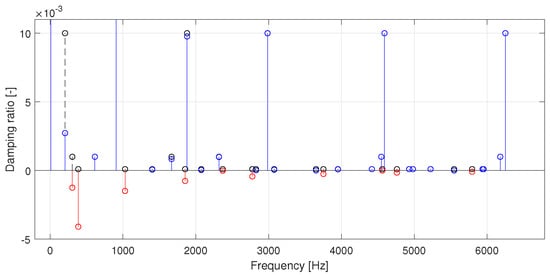
Figure 3.
Equivalent damping ratio of wheel modes with respect to frequency (black: damping ratio of the free damped wheel modes, blue: equivalent damping ratio of stable modes, red: equivalent damping ratio of unstable modes). For purposes of visualization, several modes do not appear in the graph due to their high damping.
3.3. Initial Conditions
The choice of the initial conditions based on different conditions on velocity and displacement is detailed in the following paragraphs.
3.3.1. Initial Condition on Velocity
The imposed lateral velocity at the wheel–rail interface due to the imperfect curving behavior of the rail-guided vehicle, as discussed in the introduction, is a good reference value for the vibratory velocity in curve squeal. For instance, the wheel vibrations obtained in [6] reach a limit cycle with an amplitude between the saturation velocity and the imposed lateral velocity . Considering this order of magnitude for the initial velocity , different values of disturbance , such that are proposed (cf. Equation (22)). These velocities are represented in the friction/creep law from Figure 4: a value of gives an initial velocity inside the creep zone, where the positive equivalent damping helps slow down the growth of the amplitude of the self-sustained vibrations, whereas gives a velocity in the slip zone, where the equivalent damping is negative and the contrary effect takes place; disturbance , on the other hand, gives a velocity that is closest to the quasi-static equilibrium, so that a slow growth of the self-sustained vibrations can be expected.
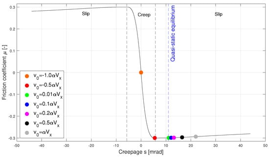
Figure 4.
Friction/creep law. Initial velocities , converted to creepage via Equation (1), are marked in color dots.
Note that in expression (22) the initial velocity is distributed over all the modes via the matrix , which translates the inertial behavior of the wheel. Figure 5 illustrates this for and it can be observed that the 0Ln modes are the ones to be excited the most with this type of initial condition.
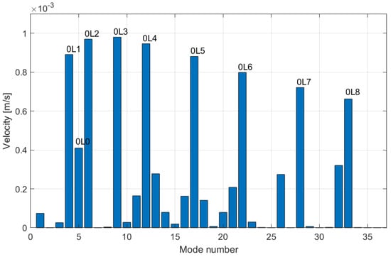
Figure 5.
Distribution of initial velocity over the modes.
3.3.2. Initial Condition on Displacement
Like for the initial condition in velocity, expression (23) distributes the perturbation over all the modes via the matrix , which translates the elastic behavior of the wheel. This is illustrated in Figure 6. It can be observed that this type of initial condition creates an excitation that is favorable to the low frequency modes, such as the wheelset modes (modes 1 to 3), as well as modes 0Ln with lower order n. Two values of the disturbance are chosen empirically, by considering a typical order of magnitude of the displacement.
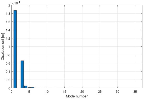
Figure 6.
Distribution of disturbance over the modes.
3.3.3. Modal-Derived Initial Conditions and Summary of the Test Cases
Taking into account the stability results, namely that 0Ln modes display the most unstable behavior, the modal initial conditions are chosen to excite the following modes:
- All unstable modes
- Mode 0Ln, with
Table 3 presents a compact overview of the initial conditions imposed to the modal contributions vector and its derivative , for all test cases, which belong to either the physically-derived initial conditions or the modal-derived ones. If unspecified, the value of the initial velocity used is .
Table 3.
Summary of the test cases.
3.4. Time Integration Results
This section discusses the results obtained after performing numerical integration in the time domain of the dynamic equations that describe the system, as presented in Section 2.1.2, and for the test cases shown in Table 3. The physical quantities that will be in the focus of the analysis are the velocity and the displacement of the wheel–rail contact point, as well as the nonlinear friction force applied to the wheel because of the imposed relative velocity between the wheel and the rail; they will be studied both in the time domain and in the frequency domain.
Figure 7 shows the evolution in time of the tangential velocity for all test cases: the first 12 cases correspond to the modal-derived initial conditions from Table 3, whereas the last 10 correspond to the physically-derived initial conditions. One can observe that velocity evolves differently in time depending on the initial condition used, which is the expected outcome of nonlinear time integration; however, inside both categories of test cases, some major features can already be outlined from these time domain results, according to the following aspects: final peak-to-peak amplitude, number of stationary regimes reached, overshoot, stabilization time and maximum amplitude.
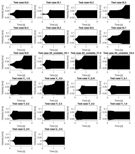
Figure 7.
Evolution of the tangential velocity at the wheel–rail contact point for all test cases from Table 3.
In general, the system seems to be able to reach two primary families of final states: a low-energy regime, with a moderate peak-to-peak amplitude of 0.1172 m/s, and a high-energy one, with an amplitude almost doubled, reaching 0.2042 m/s. Cases “0L3”, “0L7” and “0L8” stand out because they display these two types of stationary regimes with a well-defined transition between them. However, a more detailed analysis that will be presented later reveals that this apparent intermediate limit-cycle is not yet stabilized. In other cases, for instance “All_unstable_V_2.0”, the vibrations directly reach a final high-energy regime.
The existence of a low-energy and a high-energy stationary regime, observation previously made on the time history of the velocity (cf. Figure 7), is more clearly visualized in Figure 8 and Figure 9, which show the phase plot (velocity vs. displacement) of the simulations, for the physically-derived and for the modal-derived conditions, respectively. Furthermore, one can observe that the low-energy cycles display a closed, almost elliptical phase plot, which corresponds to a periodic regime with one fundamental frequency and some of its harmonics, whereas high-energy regimes display a rather complex phase plot that corresponds to a quasi-periodic regime where multiple fundamental frequencies and their harmonic interactions coexist.
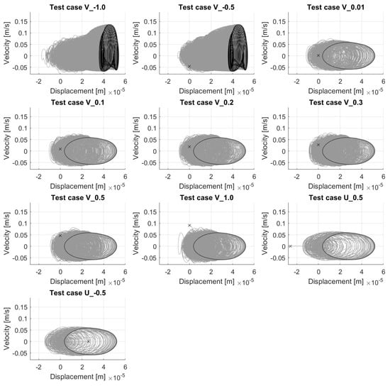
Figure 8.
Phase plot of the wheel–rail contact point for all physically-derived initial conditions from Table 3. Grey: complete history, black: final limit cycle reached, ‘x’: initial condition.
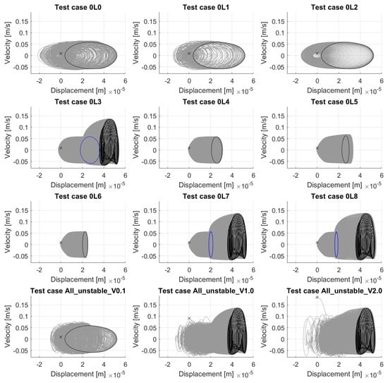
Figure 9.
Phase plot of the wheel–rail contact point for all modal-derived initial conditions from Table 3. Grey: complete history, blue: intermediate limit cycle, black: final limit cycle reached, ‘x’: initial condition.
For test case “All_unstable_V2.0” (cf. Figure 9), in which the initial velocity (marked with an “x”) is considerably higher than the maximum velocity amplitude reached during the simulation, the system is still attracted to one of the two observed stationary regimes, namely the high-energy one; the same is true for cases “U_0.5” and “U_-0.5”, which have a non-zero initial displacement, but they are attracted to a low-energy limit cycle.
An interesting remark, observed for all simulations, regardless of the initial condition used, is that the mean displacement increases gradually during the transient phase, i.e., the phase plot shifts slowly to the right. For instance, in both test cases U_0.5 and U_-0.5, which start at a non-zero displacement, the system quickly returns to the quasi-static position at , but then the mean value starts to increase until a stationary regime is reached. This is related to the inclusion of the wheelset modes (modes 1 to 3) in the wheel’s modal base, which contribute to the quasi-static behavior of the structure, due to their low natural frequency.
Figure 10 highlights an interesting result, namely, that the two families of limit cycles identified before (the low-energy and the high-energy ones) can be obtained for both physical and modal initial conditions. Depending on their value, physically-derived initial conditions can lead to either of the two, but in the first case, the same periodic limit cycle, plotted in black in Figure 10a, is always obtained. Test cases with modal initial conditions can lead to more than one unique periodic cycle, as can be seen in Figure 10b: in total, four unique periodic cycles have been identified. The quasi-periodic cycles reached for both categories of test cases correspond in reality to a unique limit cycle that tends to color the same surface in the phase plot, with each individual instance having a different translation in time.
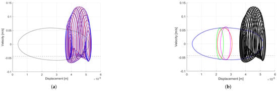
Figure 10.
Phase plot of the final limit cycles obtained for the physically-derived initial conditions (a) and the modal-derived ones (b). Creep and slip zones are below and above the dashed black line, respectively. (a): red: “V_-1.0”, blue: “V_-0.5”, black: all other physically-derived initial conditions. (b): red: “0L4”, magenta: “0L5”, green: “0L6”, black (curves superpose): “0L3”/“0L7”/“0L8”/“All_unstable_V1.0”/“All_unstable_V2.0”, blue (curves superpose): all other modal-derived initial conditions.
Figure 11 and Figure 12 show the velocity spectrum and the friction force spectrum, respectively, for all the periodic limit-cycles that were identified among all test cases regardless of the type of initial conditions used. The aforementioned unique periodic cycles have different fundamental frequencies: 1855 Hz, 2775 Hz, 3750 Hz for test cases “0L4”, “0L5”, “0L6”, respectively, which are close to the natural frequencies of the corresponding modes, and 385 Hz for all other periodic cycles, which is close to the natural frequency of mode 0L2.
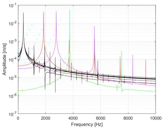
Figure 11.
FFT of the velocity of the periodic limit cycles obtained among all test cases (red: “0L4”, magenta: “0L5”, green: “0L6”, black (curves superpose): all other cases leading to a periodic limit cycle).
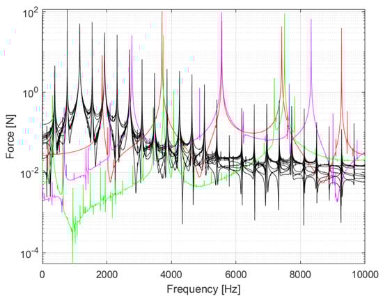
Figure 12.
FFT of the nonlinear friction force of the periodic limit cycles obtained among all test cases (red: “0L4”, magenta: “0L5”, green: “0L6”, black (curves superpose): all other test cases from Table 3).
The spectrum in Figure 13 can be considered as quasi-periodic if Hz, Hz and Hz are accepted as its fundamental, incommensurable frequencies (i.e., that have no common integer divisor). In spite of the low amplitude of the peak at , the latter is considered as a fundamental frequency because it explains some of the harmonic modulations (i.e., linear combinations of the fundamental frequencies) present in the spectrum. Notice that any two of the three high-amplitude peaks at , and could have been labeled as fundamental frequencies and an equivalent understanding of the spectrum would have been obtained.
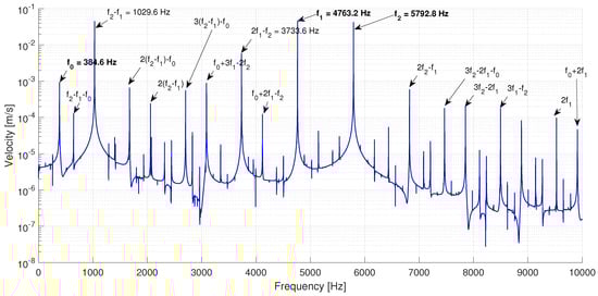
Figure 13.
FFT of the velocity of a pseudo-periodic limit cycle (test case “All_unstable_V_2”)).
For the reader’s comprehension, this spectrum can be qualified as bi-periodic with fundamental frequencies and and a secondary contribution of . Regardless, these three frequencies are close to the natural frequencies of modes 0L7, 0L8 and 0L2, respectively, and the harmonic modulations at Hz and Hz are very close to the natural frequency of modes 0L3 and 0L6, respectively. Indeed, the strong harmonic correlation between the unstable modes 0L2, 0L3, 0L6, 0L7 and 0L8 observed in this limit cycle could explain its quasi-periodic nature.
The existence of this particular quasi-periodic limit cycle illustrates the limitation of the stability analysis previously proposed in Section 3.2, which is not able to predict the appearance of some harmonic components based on the combination of the fundamental frequency of unstable modes and that end up having a strong contribution on the self-sustained oscillations. It is also observed that the most unstable mode predicted by the stability analysis (mode 0L2 with fundamental frequency of 386.4 Hz) does not have the most important contribution on the pseudo-periodic limit cycle. This reflects the nonlinear behavior of the force and interactions at the frictional interface, which the stability analysis is not able to represent.
It is also interesting to highlight the frequency shift that can be observed in the spectrum from Figure 13, in which the frequency resolution is 0.8 Hz: while the stability analysis, a linear approach, predicted unstable frequencies 386.4, 1028.8, 4762.2 and 5794.7 Hz, nonlinear time integration gave a limit cycle with frequency components at 384.6, 1029.6, 4763.2 and 5792.8 Hz; these frequencies are slightly shifted in order to interact harmonically with each other. Again, this is a feature that the stability analysis alone is not able to represent.
Figure 14 shows the evolution of the modal projections of two modal-derived test cases, “0L1” and “0L2”. Although both cases lead to a periodic limit cycle dominated by mode 0L2, the modal competition patterns are different in both cases. For instance, in test case “0L2”, one can observe that, as only the unstable mode 0L2 is excited at the beginning of the simulation, the other unstable modes remain almost at a constant level, they do not interact, giving a rather smooth evolution of the vibrations (cf. phase plot of the contact point, Figure 9). On the contrary, in test case “0L1”, where a stable mode, 0L1, is excited at the beginning of the simulation, two different stages of the time domain simulation can be clearly identified: first, a transient phase with exponential modal growth, where the slope of the curves (i.e., the modal growth rates) decreases with the order n of the unstable 0Ln mode. This behavior is in good coherence with the results from the stability analysis (cf. Figure 3), as the behavior in this phase remains linear-like. Moreover, one can observe that there is a richer interaction between the different modes in this phase, hence giving a more complex phase plot (cf. Figure 9). In the end of the transient phase, saturation is reached and all modes other than 0L2 die out, introducing the second stage, where a stabilized regime is maintained.
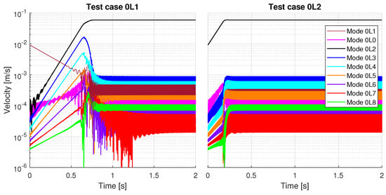
Figure 14.
Comparison of the modal projections of the unstable 0Ln modes for two modal-derived test cases (Y-scale is shared by both graphs).
Figure 15 shows the modal competition of one modal-derived case (“All_unstable_V1.0”) vs. one physically-derived case (“V_1.0”). In both cases, the initial velocity at the contact point is equal to the sliding velocity between the wheel and the rail, , but the way in which it is distributed into the different modes, in particular the unstable modes differs: in case “All_unstable_V1.0”, all unstable modes have the same starting point, whereas for the case “V_1.0”, they start at different levels, as illustrated in Figure 5. Although the initial velocity at the contact point is the same, in the first case, a quasi-periodic limit cycle is obtained, whereas a periodic one is reached for the second case. The modal competition patterns in the transient phase are different for both cases as well: in the first case, mode 0L3 dominates from the beginning, while the other modes die out rapidly; then, modes that present a harmonic correlation, namely 0L3, 0L6, 0L7 and 0L8, suddenly revert their decaying tendency and present an exponential growth until they finally reach saturation around s, where the vibrations stabilize and give a limit cycle whose signature is the one from Figure 13. In the second case, on the contrary, mode 0L2, which has the most negative equivalent damping according to the stability analysis, dominates the modal competition from the beginning and all other modes die out rapidly; this mode alone dominates the limit cycle. These results indicate that not only the global value of the initial condition, in this case the velocity at the contact point, has an impact on the nature of the final limit cycle obtained, but also the initial condition given to each particular mode.
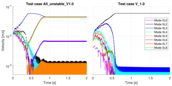
Figure 15.
Comparison of the modal projections of the unstable 0Ln modes for a modal-derived test case vs. a physically-derived test case (Y-scale is shared by both graphs).
Figure 16 shows the evolution of the modal projections of the harmonically-correlated modes for the test cases in which only one of these instabilities is excited in the initial condition (test case “0L2” is included for reference). Here, the development of a quasi-periodic cycle is more clearly visualized: while for test case “0L2” the modal projections of non-excited modes cease to grow in amplitude and stabilize completely at a certain point, in the other three test cases, the non-excited but harmonically-correlated instabilities are growing exponentially in the background, while an apparent stationary regime dominated by the initially-excited mode is reached. This is why the existence of an intermediate limit cycle, as discussed at the beginning of this section and as shown in Figure 9, could be nuanced by considering that all modes are not yet completely stabilized, which results in an apparent limit cycle that is slowly evolving to the definitive, stabilized limit cycle.
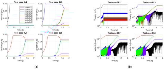
Figure 16.
Comparison of the modal projections of unstable 0Ln modes for test cases “0L2”, “0L3”, “0L7”, “0L8”, linear scale (a) and logarithmic scale (modes other than 0L3, 0L6, 0L7, 0L8 have been removed for visualization purposes) (b).
From test case “All_unstable_V1.0” (Figure 15) and test cases “0L3”, “0L7” and “0L8” (Figure 16) it can be pointed out that the harmonic correlation phenomenon between modes in order to give birth to a quasi-periodic limit cycle occurs after saturation of the friction has taken place, so that the nonlinear domain of the friction law is fully established. This implies that in this stage, the modal growth rates of modes such as 0L6, 0L7, 0L8, no longer correspond to that predicted by the stability analysis, which is the case of the linear phase in test case “0L1” from Figure 14: the slopes of the curves differ.
In summary, physically-derived initial conditions lead to only two scenarios: either a periodic limit cycle with a moderate peak-to-peak amplitude, or a quasi-periodic limit cycle with a higher peak-to-peak amplitude. The same two cycles (one periodic and the other quasi-periodic) were always obtained. In addition, the results suggest that the appearance of the quasi-periodic limit cycle is related to initial conditions quite far from the quasi-static equilibrium. On the other hand, modal-derived initial conditions lead to more scenarios: the same quasi-periodic cycle as that obtained with physically-derived initial conditions but several periodic limit cycles with different fundamental frequencies (related to the modal content of initial conditions). Thus, it is worth noting that some periodic limit cycles could only be obtained with modal initial conditions and not with physically-derived ones. Moreover, contrary to the case of physical-derived initial conditions, the quasi-periodic limit cycle can be obtained with initial conditions close to the quasi-static equilibrium but with a specific modal content.
4. Conclusions
The impact of initial conditions on the limit cycles obtained with time integration for a curve squeal model based on the falling friction instability mechanism was studied in this paper. Two types of initial conditions were used, the modal-derived and the physically-derived ones and, in order to implement the latter, a formulation allowing to relate a physical initial condition on velocity and on displacement to its equivalent initial modal contributions was presented.
The limit cycles that were obtained for both types of initial conditions were found to belong to either of two primary families: on the one hand, low-energy cycles with a moderate peak-to-peak amplitude and a periodic regime and, on the other hand, high-energy cycles with a high amplitude, almost doubling that of the low-energy ones, and presenting a quasi-periodic regime. It was shown that, irrespective of the initial conditions, the cases where a quasi-periodic regime was obtained converged to a same unique limit cycle, which displays three fundamental frequencies, corresponding to specific 0Ln wheel modes. High amplitude peaks were identified at some harmonic interactions among these modes, which corresponded as well to specific wheel modes. In order for this type of cycle to develop, it was observed that the natural frequencies of the concerned unstable modes slightly shifted with respect to the frequencies predicted by the stability analysis; this kind of feature is typical of nonlinear systems and cannot be fully addressed by a stability analysis.
It was shown that exciting a specific unstable mode at the beginning of the simulation could lead in some cases to a periodic limit cycle with a fundamental frequency corresponding to that particular mode. However, in other cases where a specific mode was excited, it was obtained either a periodic limit cycle with fundamental frequency close to a different unstable mode, or a quasi-periodic cycle with multiple fundamental frequencies, corresponding to the natural frequencies of specific wheel modes that have a strong harmonic correlation. Moreover, due to this harmonic coupling, these specific modes are not able to exist alone in a limit cycle, because of their strong interaction. Physically-derived initial conditions, on the other hand, such as an imposed initial velocity or displacement at the contact point, led either to a unique periodic limit cycle, in which the fundamental frequency corresponds to the most unstable mode identified by the stability analysis, or to a unique quasi-periodic limit cycle (the same found for the modal-derived initial conditions).
The results presented in this paper stress the importance of an adequate choice of the initial conditions when it comes to the study of curve squeal via time integration methods, and more generally the field of friction-induced vibrations. The nonlinear nature of these phenomena introduces some complexities, such as a strong dependence of the final limit cycle to the initial conditions, as well as harmonic coupling between specific modes of the structure. It is worth studying these aspects in detail, not only in order to have a better understanding and control of the initial conditions on the final results, but also to produce more robust and reliable simulations, which is of great interest for industrial purposes in particular. Finally, future developments allowing for the correlation of time integration results to those obtained with direct nonlinear methods would help deepen the understanding of the problem treated in the present study.
Author Contributions
Conceptualization, J.A.M., O.C., J.-J.S. and R.T.; Methodology, J.A.M., O.C., J.-J.S. and R.T.; Software, J.A.M. and O.C.; Validation, J.A.M., O.C., J.-J.S. and R.T.; Investigation, J.A.M., O.C., J.-J.S. and R.T.; Data curation, J.A.M. and O.C.; Writing—original draft, J.A.M.; Writing—review & editing, J.A.M., O.C., J.-J.S. and R.T.; Visualization, J.A.M.; Supervision, O.C., J.-J.S. and R.T. All authors have read and agreed to the published version of the manuscript.
Funding
This research received no external funding.
Data Availability Statement
The raw data supporting the conclusions of this article will be made available by the authors on request.
Acknowledgments
This work was performed within the framework of the LABEX CeLyA (ANR-10-LABX-0060) of Université de Lyon, within the program « Investissements d’Avenir » operated by the French National Research Agency (ANR).
Conflicts of Interest
Author Jacobo Arango Montoya and Rita Tufano were employed by the company Vibratec. The remaining authors declare that the research was conducted in the absence of any commercial or financial relationships that could be construed as a potential conflict of interest.
References
- Thompson, D.J.; Squicciarini, G.; Ding, B.; Baeza, L. A State-of-the-Art Review of Curve Squeal Noise: Phenomena, Mechanisms, Modelling and Mitigation. In Noise and Vibration Mitigation for Rail Transportation Systems; Notes on Numerical Fluid Mechanics and Multidisciplinary Design; Springer: Cham, Switzerland, 2018; pp. 3–41. [Google Scholar] [CrossRef]
- Rudd, M.J. Wheel/rail noise—Part II: Wheel squeal. J. Sound Vib. 1976, 46, 381–394. [Google Scholar] [CrossRef]
- van Ruiten, C.J.M. Mechanism of squeal noise generated by trams. J. Sound Vib. 1988, 120, 245–253. [Google Scholar] [CrossRef]
- Fingberg, U. A model of wheel-rail squealing noise. J. Sound Vib. 1990, 143, 365–377. [Google Scholar] [CrossRef]
- de Beer, F.G.; Janssens, M.H.A.; Kooijman, P.P. Squeal noise of rail-bound vehicles influenced by lateral contact position. J. Sound Vib. 2003, 267, 497–507. [Google Scholar] [CrossRef]
- Chiello, O.; Ayasse, J.B.; Vincent, N.; Koch, J.R. Curve squeal of urban rolling stock—Part 3: Theoretical model. J. Sound Vib. 2006, 293, 710–727. [Google Scholar] [CrossRef]
- Hoffmann, N.; Fischer, M.; Allgaier, R.; Gaul, L. A minimal model for studying properties of the mode-coupling type instability in friction induced oscillations. Mech. Res. Commun. 2002, 29, 197–205. [Google Scholar] [CrossRef]
- Glocker, C.; Cataldi-Spinola, E.; Leine, R.I. Curve squealing of trains: Measurement, modelling and simulation. J. Sound Vib. 2009, 324, 365–386. [Google Scholar] [CrossRef]
- Pieringer, A. A numerical investigation of curve squeal in the case of constant wheel/rail friction. J. Sound Vib. 2014, 333, 4295–4313. [Google Scholar] [CrossRef]
- Ding, B.; Squicciarini, G.; Thompson, D. Effect of rail dynamics on curve squeal under constant friction conditions. J. Sound Vib. 2019, 442, 183–199. [Google Scholar] [CrossRef]
- Lai, V.V.; Chiello, O.; Brunel, J.F.; Dufrénoy, P. The critical effect of rail vertical phase response in railway curve squeal generation. Int. J. Mech. Sci. 2020, 167, 105281. [Google Scholar] [CrossRef]
- Jiang, J.; Anderson, D.C.; Dwight, R. The Mechanisms of Curve Squeal. In Noise and Vibration Mitigation for Rail Transportation Systems; Notes on Numerical Fluid Mechanics and Multidisciplinary Design; Springer: Berlin/Heidelberg, Germany, 2015; pp. 587–594. [Google Scholar] [CrossRef]
- Meehan, P.A. Prediction of wheel squeal noise under mode coupling. J. Sound Vib. 2020, 465, 115025. [Google Scholar] [CrossRef]
- Huang, Z.Y.; Thompson, D.J.; Jones, C.J.C. Squeal Prediction for a Bogied Vehicle in a Curve. Noise and Vibration Mitigation for Rail Transportation Systems; Springer: Berlin/Heidelberg, Germany, 2008; pp. 313–319. [Google Scholar] [CrossRef]
- Ding, B.; Squicciarini, G.; Thompson, D.; Corradi, R. An assessment of mode-coupling and falling-friction mechanisms in railway curve squeal through a simplified approach. J. Sound Vib. 2018, 423, 126–140. [Google Scholar] [CrossRef]
- Charroyer, L.; Chiello, O.; Sinou, J.J. Self-excited vibrations of a non-smooth contact dynamical system with planar friction based on the shooting method. Int. J. Mech. Sci. 2018, 144, 90–101. [Google Scholar] [CrossRef]
- Coudeyras, N.; Nacivet, S.; Sinou, J.J. Periodic and quasi-periodic solutions for multi-instabilities involved in brake squeal. J. Sound Vib. 2009, 328, 520–540. [Google Scholar] [CrossRef]
- Zenzerovic, I. Time-Domain Modelling of Curve Squeal: A Fast Model for One- and Two-Point Wheel/Rail Contact. Ph.D Thesis, Chalmers University of Technology, Gothenburg, Sweden, 2017. ISBN 9789175976471. [Google Scholar]
- Ding, B. The Mechanism of Railway Curve Squeal. Ph.D Thesis, University of Southampton, Southampton, UK, 2018. [Google Scholar]
- Loyer, A.; Sinou, J.J.; Chiello, O.; Lorang, X. Study of nonlinear behaviors and modal reductions for friction destabilized systems. Application to an elastic layer. J. Sound Vib. 2012, 331, 1011–1041. [Google Scholar] [CrossRef][Green Version]
- Lai, V.V.; Anciant, M.; Chiello, O.; Brunel, J.F.; Dufrénoy, P. A nonlinear FE model for wheel/rail curve squeal in the time-domain including acoustic predictions. Appl. Acoust. 2021, 179, 108031. [Google Scholar] [CrossRef]
- Heckl, M.A.; Abrahams, I.D. Curve squeal of train wheels, part 1: Mathematical model for its generation. J. Sound Vib. 2000, 229, 669–693. [Google Scholar] [CrossRef]
- Giner-Navarro, J.; Martínez-Casas, J.; Denia, F.D.; Baeza, L. Study of railway curve squeal in the time domain using a high-frequency vehicle/track interaction model. J. Sound Vib. 2018, 431, 177–191. [Google Scholar] [CrossRef]
- Schneider, E.; Popp, K.; Irretier, H. Noise generation in railway wheels due to rail-wheel contact forces. J. Sound Vib. 1988, 120, 227–244. [Google Scholar] [CrossRef]
- Thompson, D.J. Railway Noise and Vibration: Mechanisms, Modelling and Means of Control; Elsevier: Amsterdam, The Netherlands, 2009. [Google Scholar]
- Ding, B.; Squicciarini, G.; Thompson, D.J. Effects of rail dynamics and friction characteristics on curve squeal. J. Phys. Conf. Ser. 2016, 744, 012146. [Google Scholar] [CrossRef]
- Kalker, J.J. Wheel-rail rolling contact theory. Wear 1991, 144, 243–261. [Google Scholar] [CrossRef]
- Shen, Z.Y.; Hedrick, J.K.; Elkins, J.A. A Comparison of Alternative Creep Force Models for Rail Vehicle Dynamic Analysis. Vehicle System Dynamics; Taylor & Francis: Abingdon, UK, 1983; Volume 12, pp. 79–83. [Google Scholar] [CrossRef]
- Newmark, N.M.; Asce, F. A method of computation for structural dynamics. J. Eng. Machanics Div. 1959, 85, 67–94. [Google Scholar] [CrossRef]
- Géradin, M.; Rixen, D. Mechanical Vibrations: Theory and Application to Structural Dynamics, 2nd ed.; Wiley: Hoboken, NJ, USA, 1997. [Google Scholar]
Disclaimer/Publisher’s Note: The statements, opinions and data contained in all publications are solely those of the individual author(s) and contributor(s) and not of MDPI and/or the editor(s). MDPI and/or the editor(s) disclaim responsibility for any injury to people or property resulting from any ideas, methods, instructions or products referred to in the content. |
© 2025 by the authors. Licensee MDPI, Basel, Switzerland. This article is an open access article distributed under the terms and conditions of the Creative Commons Attribution (CC BY) license (https://creativecommons.org/licenses/by/4.0/).