Abstract
In the interior decoration panel industry, automated production lines have become the standard configuration for large-scale enterprises. However, during the panel processing procedures such as sanding and painting, the loss of traditional identification markers like QR codes or barcodes is inevitable. This creates a critical technical bottleneck in the assembly stage of customized or multi-model parallel production lines, where identifying individual panels significantly limits production efficiency. To address this issue, this paper proposes a high-precision measurement method based on close-range photogrammetry for capturing panel dimensions and hole position features, enabling accurate extraction of identification markers. Building on this foundation, an identity discrimination method that integrates weighted dimension and hole position IDs has been developed, making it feasible to efficiently and automatically identify panels without physical identification markers. Experimental results demonstrate that the proposed method exhibits significant advantages in both recognition accuracy and production adaptability, providing an effective solution for intelligent manufacturing in the home decoration panel industry.
1. Introduction
As leading home decoration panel enterprises like JOMOO advance intelligent manufacturing upgrades, the automated production line for bathroom cabinet panels is gradually becoming widespread [1]. The automated production line has become a key tool for achieving efficient production in the home decoration panel industry, particularly in the production of bathroom cabinet panels, where traditional manual operations are gradually being replaced by automated systems to improve production efficiency, reduce costs, and ensure product quality. However, technical bottlenecks still exist in practical applications, especially in the panel processing stage. Due to processes such as sanding and painting, traditional identification information like QR codes and barcodes are often damaged, making subsequent automatic identification and sorting difficult [2]. Especially in the customized production model with multiple parallel product types, where there are numerous panel varieties and similar dimensions, traditional label recognition methods fail to meet the needs for efficient, accurate, and flexible production. Therefore, achieving high-precision automated panel identification without labels has become a technical challenge that the home decoration panel industry urgently needs to address.
As illustrated in Figure 1, in the absence of effective automatic identification methods, the current production line still primarily relies on manual measurement and comparison of panel three-dimensional data for sorting. This not only leads to low efficiency but also introduces significant errors, severely limiting the overall automation level of the production line [3].
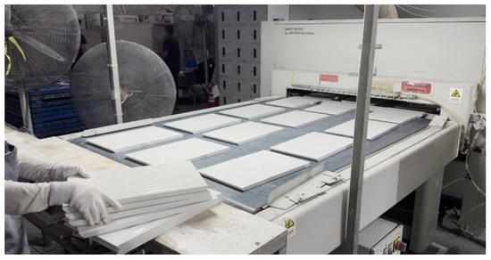
Figure 1.
The schematic diagram of the JOMOO panel production line sorting site.
Currently, methods based on computer vision and deep learning have been widely applied in the field of industrial automation, particularly in defect detection and automatic sorting systems. YOLO series models have become an important tool for industrial identification due to their outstanding accuracy and speed [4,5,6]. However, these methods typically rely on large amounts of labeled data and substantial computational resources and perform poorly in the face of environmental changes such as lighting, occlusion, reflection, and label damage. Particularly in noisy production environments, recognition performance can significantly degrade [7]. Therefore, despite significant progress in visual recognition methods, many practical challenges remain.
Additionally, in complex production environments, external factors such as lighting variations, vibrations, and high-reflectivity surfaces can significantly affect the accuracy of traditional visual recognition methods [8]. For example, uneven lighting can cause variations in image brightness, vibrations can lead to image blurring, and reflective surfaces can interfere with image quality, thereby affecting feature extraction and object localization [9]. To address these challenges, close-range photogrammetry technology has gradually become an effective solution. By extracting geometric features from images, close-range photogrammetry not only enables high-precision three-dimensional measurement and object identification without physical labels but also operates without human intervention. This technology can stably perform precise object localization and identification in dynamic and complex production environments, avoiding the instability associated with traditional methods.
Existing photogrammetry technologies typically rely on complex calibration processes and require high stability and adaptability in dynamic production environments, which limits their widespread application [10]. Particularly in dynamic environments, factors such as vibration and lighting changes can affect the accuracy of photogrammetry, leading to significant measurement errors that, in turn, impact the precision of object localization and identification [11]. To address this, this paper proposes a label-free panel recognition method based on close-range photogrammetry, aiming to overcome the limitations of traditional technologies in dynamic environments. Compared to traditional computer vision and deep learning methods, the approach proposed in this paper does not require precise component alignment, simplifying the data preprocessing process and significantly enhancing the system’s processing efficiency and adaptability.
2. Identity Recognition Method for Home Decoration Panels Based on Composite Weighting of Dimension and Hole IDs
On the JOMOO bathroom cabinet panel production line, panels generally lack usable identity markers upon entering the sorting stage, as labels are easily damaged during processing. Traditional methods rely on manual measurement of panel dimensions followed by comparison with design drawings for sorting, which is both inefficient and error-prone, making them inadequate for the high-paced demands of customized production.
To address this issue, the present study proposes a composite weighted recognition method that integrates dimension IDs and hole IDs. By extracting key geometric features of panels through close-range photogrammetry, this approach enables high-precision automated identification under unlabeled conditions. The principle of the visual measurement system, as shown in Figure 2, includes the key geometric features of the panels, which are as follows: the dimension ID, consisting of three attributes—length (A), width (B), and height (C); and the hole ID, defined using a specific matching method parameter (D).
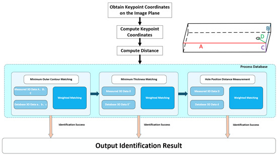
Figure 2.
Principle of Visual Measurement System.
2.1. Dimension ID Matching Method
To implement the panel automated identification system under unlabeled conditions, as illustrated in Figure 3, the minimum enclosing contour and minimum thickness contour of panels in the images must first be automatically extracted. The LSD algorithm is employed to extract the intersection coordinates of edge line segments [12,13], obtaining the key corner point coordinates in the image plane [14]. The corresponding object-space coordinates are then computed using the collinearity equations, after which the length, width, and height metrics are calculated and compared against the database.
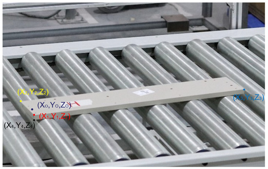
Figure 3.
Key point diagram of the panel.
For the measured panel length the error is calculated by comparing it with the corresponding reference value from the database using the following formula:
where represents the error between the measured value and the database value. The calculated is then compared with a preset threshold, , which should be set at 1% of the dimension of the measured object.
If , the matching weight of the corresponding database drawing is increased by 1. This comparison process is applied separately to the length, width, and height of the panel. After completing the comparisons for all dimensions, the final matching is performed in the database based on the accumulated matching weights for each metric, with the drawing exhibiting the highest total matching weight selected as the best match.
Some panels exhibit segmented edge thickness characteristics, with the front section maintaining a vertical height and the rear section transitioning in a wedge-shaped manner, which prevents a single measurement from accurately reflecting the true panel thickness. To address this, the system employs a multi-point thickness localization strategy, extracting key points at specific locations and calculating multiple thickness metrics , etc., thereby avoiding errors from single-point measurements and ensuring accurate representation of complex panel geometries. After converting image coordinates to object-space coordinates, precise measurements of panel length, width, and multi-segment edge thickness are performed to construct a panel dimension feature vector, forming a reliable dimension ID.
2.2. Hole ID Matching Method
When the dimension ID is duplicated or cannot uniquely identify the panel, the system introduces hole features as an auxiliary criterion. Due to significant differences in the number, position, and distribution of holes across different panels, the system performs matching based on the spatial location information of the holes [15,16]. Specifically, the system locates the hole features in the image using the center recognition algorithm of YOLOv8n. First, the Hough transform is used to extract circular features from the image, a method that effectively identifies the circular edges and extracts the center of the circle. Subsequently, the YOLOv8n model is used for precise localization of the center positions, which are treated as key features. The system further calculates the geometric distance from the hole center to the nearest corner point and uses this distance as a spatial geometric feature for the subsequent auxiliary judgment process.
As shown in Dimension Index Table 1.

Table 1.
ID parameter table.
The calculation process is as follows:
where
- denote the image coordinates of the principal point;
- represent the camera center coordinates;
- and are parameters obtained from camera calibration.
In the calculation of length and width metrics, as illustrated in Figure 3:
To further analyze the distances between panel features (such as hole positions) and key corner points:
where points and represent the coordinates of the key points, while point denotes the coordinates of the center of the circular hole.
Ultimately, the system performs a weighted fusion of dimension and hole features to generate a unique identity, which is then used for comparison with the standard panel database. This method does not require physical labels and achieves high identification accuracy, making it suitable for the automated sorting of panels with multiple specifications and without markings. However, in actual production line environments, factors such as vibration, noise, and optical distortion of the camera lens can affect recognition accuracy. Therefore, although the feature-weighted fusion method exhibits high accuracy in theory, to address the instability factors present in production line environments, this study proposes a control-point and pointer-point weighted selection method based on an optical distortion model to further enhance calibration precision.
3. High-Precision Focal Length Calibration Method Based on the Principle of Global Scanning
3.1. Close-Range Photogrammetry Method
Close-range photogrammetry is a three-dimensional reconstruction method based on camera imaging principles [17]. As illustrated in Figure 4, the principle of ray intersection serves as the foundation for computing object-space coordinates [18]. By performing back intersection using known control points, the camera’s spatial position and orientation can be recovered to obtain the exterior orientation elements [19,20]. Subsequently, corresponding image points are identified across multiple images, their image-plane coordinates are extracted, and the imaging ray directions are reconstructed based on geometric relationships [21]. By exploiting the reversibility of light rays, multi-view rays are back-projected and intersected to obtain the three-dimensional coordinates of object points, thereby achieving reconstruction from two-dimensional images to a three-dimensional real scene [22]. In this study, this method is employed to extract panel contours and hole features, offering high accuracy, flexible deployment, and strong adaptability, and providing a reliable data foundation for subsequent identification.
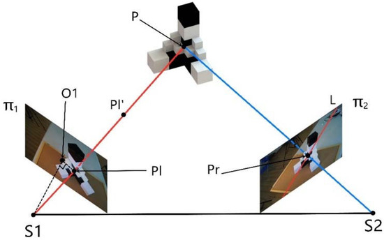
Figure 4.
Schematic diagram of photogrammetry calculation principle.
The accuracy of photogrammetry largely depends on the precision of the focal length. However, in the field environment of automated panel production lines, factors such as vibration and displacement can induce slight variations in the camera’s focal length, thereby affecting the accuracy of three-dimensional reconstruction. A field calibration method is required to ensure both recognition accuracy and system real-time performance. In this study, a high-precision focal length calibration method based on the principle of global scanning is proposed, enabling rapid and adaptive correction of the focal length.
The calibration principle involves using the collinearity equations of photogrammetry to perform forward intersection and compute the camera’s interior orientation elements . When the exterior orientation elements, object-space coordinates, and interior orientation elements are distinguished, the formulation [23] can be expressed as follows:
Through numerical simulation analysis in the author’s doctoral dissertation, it was demonstrated that slight variations in the focal length have a significant impact on measurement errors [24]. As shown in Figure 5, the simulation results reveal the relationship between focal length within a certain range and measurement accuracy. By performing a global scan within the possible range of focal length values and selecting the value that minimizes the error, this approach embodies the principle of global scanning.
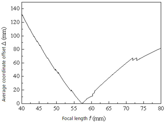
Figure 5.
f-Δ relationship diagram.
Each additional measurement image provides a collinearity equation as shown in Equation (6). When the number of measurement images satisfies , the linearized collinearity equation system can be used to compute the object-space coordinates of points corresponding to the identified image points. By incorporating redundant data, the focal length calibration error caused by random errors in the reference measurements can be minimized to the greatest extent [25].
Let us consider check points set for the same camera-lens combination. Using the single-point focal length scanning calibration model with identical iteration steps and step sizes, single-point focal length scanning calibration models can be computed. In this case, to select the focal length corresponding to the minimum error, the focal length deviations at each scanning step for all check points are combined into a comprehensive error set . This set is referred to as the multi-point focal length scanning calibration model:
Let the minimum value corresponding to be
The focal length calibration value corresponding to the multi-point focal length scanning calibration model is then
3.2. A Weighted Selection Method for Control Points Based on Optical Distortion Model
3.2.1. Optical Distortion Model
To further enhance the accuracy of the calibration results, this study proposes a weighted algorithm based on the camera lens optical distortion model to optimize calibration errors caused by lens distortion. The distortion errors of optical lenses primarily include radial distortion, decentering distortion, and thin-prism distortion [26]. According to the studies by Ricolfe-Viala C [27] et al., the optical lens distortion model can be divided into a distortion model along the x-axis and a distortion model along the y-axis:
where and are the combined values of nonlinear distortion in the x-axis and y-axis directions of the image-plane coordinate system; and are the radial distortion parameters in the x-axis and y-axis directions; and and are the decentering distortion parameters in the x-axis and y-axis directions of the image-plane coordinate system. and are the thin-prism distortion parameters in the x-axis and y-axis directions of the image-plane coordinate system; and are radial distortion coefficients; and are decentering distortion coefficients; and and are thin-prism distortion coefficients. The spatial relationships of and within the image-plane coordinate system are illustrated in Figure 6.
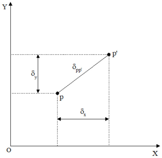
Figure 6.
The spatial relationship of the image plane coordinate system.
In the automated identification system for bathroom cabinet panels, calculating the optical distortion of the camera lens is a fundamental step for achieving accurate measurements and three-dimensional reconstruction. Although the cameras used in this system are not industrial-grade professional measurement devices, mid-to-high-end DSLR cameras such as the Canon 5Ds and their original lenses are typically employed. These devices offer manufacturing and assembly precision sufficient to meet the requirements of demanding engineering applications. Therefore, based on the theory proposed by Ricolfe-Viala C and colleagues, the optical distortion calculation model for this type of equipment can be moderately simplified, retaining the first-order radial distortion and second-order decentering distortion of the lens [28,29]:
Here, ; are the coordinates of the camera principal point; and , and , are the radial and decentering distortion coefficients, respectively. Based on the above model, the optical distortion of the lens at each point results in different calibration outcomes and the confidence of the image point is given by
Let there be check points and s images used in the calculation process. According to Equation (11), the optical distortion error at each point in the image-plane coordinate system can be computed, forming the following error set:
Based on Equation (12), the combined distortion error of each image point can be calculated, and the error weight coefficient for each image point is thus defined. The weight coefficients for all points are
Considering that the numerical ranges of weights at different positions may vary significantly, the above weight coefficients are normalized to ensure computational stability and comparability, mathematically expressed as
Subsequently, the above weight coefficients are incorporated into the focal length scanning calibration model to construct a weighted multi-point focal length calibration model, as shown in Equation (15):
During the calibration process, to determine the optimal focal length position, the weighted focal length variation at all positions under the influence of the weights must be calculated, and the minimum value is selected:
Finally, based on the optimal scanning step , reference focal length , maximum offset of the scanning range , and total number of scanning steps n, the actual focal length value for that step is calculated as
3.2.2. Control Point Selection Method
The selection of control points should follow the principle of optimal distribution in theory, in order to ensure the stability and accuracy of the calibration solution13. In theory, the number of control points should be no less than four to avoid introducing significant numerical errors during the Newton iteration process. However, an excessive number of control points may increase the instability of the model fitting. Therefore, in this study, a total of six control points were selected. In the actual measurement environment of the production line, continuous vibrations generated by equipment operation can cause significant fluctuations in the control point data collected by the total station, thereby increasing measurement errors. To mitigate the impact of vibration interference, this study excluded the set of control points with the largest data variation, thereby removing the most unstable data.
Subsequently, during the distortion analysis process, we considered factors such as mirror distortion, tangential distortion, and wave-prism distortion. Zhenyou Zhang’s calibration method was employed to fit the distortion parameters for each set of control points. Although this method may experience numerical fluctuations in a single calculation, it can still serve as an evaluation metric in continuous multiple measurements. Through the consistency analysis of multiple calibration results, we confirmed that although some control point combinations exhibited fluctuation, their corresponding average distortion values were significantly smaller than those of other combinations. Therefore, they were selected as the final set of control points.
4. Verification Experiment
4.1. Experiment Procedure
To validate the feasibility of the methods described in Section 2 and Section 3, and to facilitate the verification of the panel identification program’s results in the panel production line environment, a verification experiment was designed, as shown in the process diagram in Figure 7.
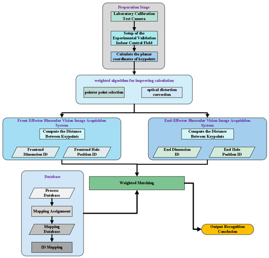
Figure 7.
Experiment procedure diagram.
As shown in Figure 7, in the simulation experiment:
The experiment introduces an optical distortion weighting mechanism, combined with Zhenyou Zhang’s calibration method, to obtain the mirror distortion, tangential distortion, and nonlinear distortion values for each control point. Based on the principle of distortion minimization, five control points with the smallest average distortion were selected from multiple candidates to avoid instability issues caused by too few points. Additionally, a pointer-point weighting strategy was applied to further improve the accuracy of the final solution.
4.2. Preparation Stage
4.2.1. Calibration Experiment Camera
The camera used in this experiment is a high-resolution DSLR, the Canon EOS 5Ds, paired with the Canon EF 50 mm f/1.8 STM lens. The technical specifications of the camera are provided in Table 2.
Table 2.
Experimental camera parameters.
To ensure the relative stability of the focal length during the experiment and the clarity of the photos used for calibration, the photos for calibration and experimental purposes were taken by first using the autofocus mode (AF) to achieve focus, and then switching to manual focus mode (MF) for capturing the images.
The camera calibration tool used in this experiment is the MATLAB-2015b Camera Calibrator toolbox.
4.2.2. Setup of the Indoor Verification Control Field
To facilitate the verification of the algorithms described in this paper within a laboratory environment and support the theoretical development and program implementation, an indoor control field was designed, as shown in Figure 8. The field possesses the following characteristics.
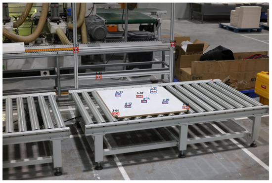
Figure 8.
Indoor Control Field Diagram.
In this experiment: Points 1-01, 2-06, 3-04, 4-05, 5-15, and 6-02 are the control points; Points a-14, b-13, c-11, d-12, and e-09 are the pointer points, used for the calculation.
Two sets of measurement data were selected as experimental subjects. The three-dimensional coordinates of each control point and test point are shown in Table 3 and Table 4. The filtered coordinates are shown in Table 5. To address measurement fluctuations caused by vibrations, the system employs a control point weighting and selection strategy. This approach eliminates the point group with the largest fluctuation, while ensuring reasonable point distribution, thus improving the stability of the solution. This method does not require additional hardware and is suitable for high-precision measurement tasks in field environments.
Table 3.
First total station measurement of accurate object coordinates for each point.
Table 4.
Second total station measurement of accurate object coordinates for each point.
Table 5.
The corrected precise coordinates of each point.
4.2.3. Capture Test Images
According to classical photogrammetry methods, two photos are required to calculate the object-space coordinates of the points to be measured, namely the left and right photos. Based on the experimental process in Figure 4, the first set of photos is taken after focusing, followed by re-focusing to capture the second set of photos. The photos used for the calculation are shown in Figure 9.
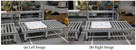
Figure 9.
Simulation verification image.
According to the data quality requirements set by industrial-grade standards, the difference between the calculated coordinates and those measured by the total station should meet the threshold selected based on 1% of the object’s size grade:
The selection criteria for the experimental thresholds are shown in Table 6.
Table 6.
Selection criteria for experiment thresholds.
During the calibration process, the distortion-weighted search range is set from 20 to 80 mm, with a total of 300 iterations (steps). Control point selection is performed after the focal length zooming in the distortion-weighted calibration, with the search range set to . The distortion weighting and the real-time calibration focal length values and , based on distortion-weighted pointer-point weighting simulation verification, are shown in Table 7.
Table 7.
Focal length calibration results.
Based on the data in Table 3, Table 5, and Table 8, and using classical photogrammetry methods, the exterior orientation elements of each camera center before and after the pointer-point selection process are calculated and are presented in Table 9 and Table 10, respectively.
Table 8.
Image plane coordinates of each point in the photo simulation experiment.
Table 9.
Exterior orientation calculation results before pointer point selection.
Table 10.
Exterior orientation calculation results after pointer point selection.
4.2.4. Calculation of Check Point Coordinates
According to the process shown in Figure 4, after zooming, traditional methods are used for calculation. The results of the calibration experiment before and after introducing the pointer-point selection method are presented in Table 11 and Table 12, respectively.
Table 11.
Calculation Results Before Pointer Point Selection.
Table 12.
Calculation Results after Pointer Point Selection.
4.2.5. Calculation Results and Discussion
By subtracting the point distances measured in Table 3 and Table 5 from the point distances measured by the total station in Table 11 and Table 12, the measurement errors of the simulation validation experiment, as shown in Table 13 and Table 14, can be obtained. In the tables, , and represent the errors between the coordinates of each test point and the true values in the measurement results before control point selection, while , and represent the errors after control point selection.
Table 13.
Calculation errors before pointer point selection.
Table 14.
Calculation errors after pointer point selection.
represent the comprehensive errors of the distances between each check point and the true values. The comprehensive errors of the calculations are shown in Table 15 and Table 16. Their calculation methods are shown in the following formulas. The error comparison is shown in Figure 10:
Table 15.
Verification results before pointer point selection.
Table 16.
Verification results after pointer point selection.
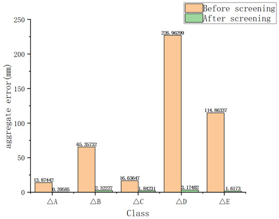
Figure 10.
Comparison of Distance Measurement Errors.
4.3. Panel Identification Program
As shown in Figure 11, to achieve high-precision identification of panels in the absence of labels, this project has developed an automatic identification system based on the fusion of hole position features and size information. The system employs close-range photogrammetry technology to extract spatial feature data and integrates optical distortion weighting and a weighted algorithm for control point selection, successfully enabling accurate classification and matching of multiple panel models in complex production environments.
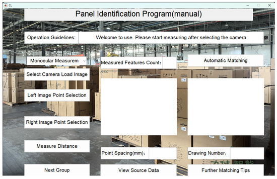
Figure 11.
System User interface.
For example, using the left partition panel:
First, select “Binocular Measurement” to switch to stereo measurement. Then, click “Select Camera Load Image” to load the camera images, and choose the left and right images of the panel to be measured, as shown in Figure 12 and Figure 13.
Figure 12.
Selection of the left image for the panel.
Figure 13.
Selection of the right image for the panel.
After selecting the left and right images of the panel to be measured, click “Left/Right Image Point Selection” to automatically extract key points from the left and right images (Figure 14). Taking the panel length A as an example, the system automatically extracts the planar two-dimensional coordinates of the key corner points.
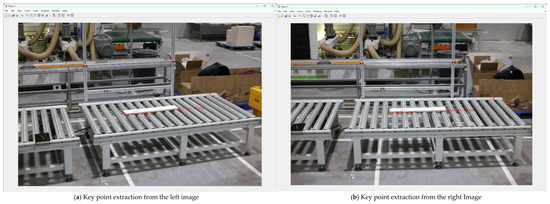
Figure 14.
Automatic Selection of Key Points for three-dimensional dimensions.
Research manuscripts reporting large datasets that are deposited in a publicly available database should specify where the data have been deposited and provide the relevant accession numbers If the accession numbers have not yet been obtained at the time of submission, please state that they will be provided during review. They must be provided prior to publication.
Next, click “Measure Distance” to measure the panel’s length A, with the measurement results shown in Figure 15.
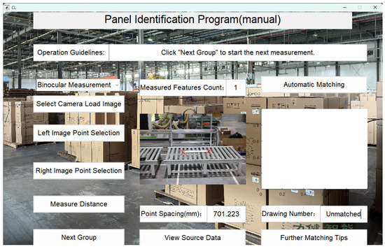
Figure 15.
Measurement results of three-dimensional data A.
After obtaining the three-dimensional dimensions (length, width, and height), select “Automatic Matching” for the first round of automatic matching. If the matching is successful, the matching results will be output, as shown in Figure 16.
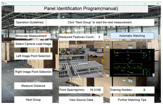
Figure 16.
Three-dimensional dimension matching result.
If the matching fails, selecting “Next Group” will automatically proceed to the next group for matching the minimum thickness and hole position distance. Since the right panel does not have a wedge-shaped edge, it will directly perform hole position distance measurement. The automatic selection of hole position key points and the distance matching results are shown in Figure 17 and Figure 18.
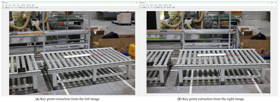
Figure 17.
Automatic selection key points for circle center.

Figure 18.
Hole ID matching result.
Taking the hollow surface as an example, the system will automatically measure the minimum thickness of its wedge-shaped edge. The automatic point selection and measurement results are shown in Figure 19 and Figure 20.
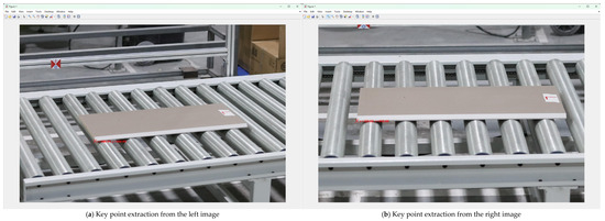
Figure 19.
Automatic selection of key points for minimum thickness.
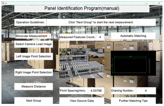
Figure 20.
Panel Minimum thickness matching result.
After obtaining the matching results, selecting “View Source Data” will allow you to view the various encoded parameters of the original blueprint.
The recognition program has been fully tested and verified on the JOMOO bathroom cabinet panel production line. The verification results are shown in Figure 21, Figure 22, Figure 23, Figure 24, Figure 25, Figure 26, Figure 27, Figure 28, Figure 29, Figure 30, Figure 31, Figure 32 and Figure 33, with the recognition accuracy reaching 100%. Through the precise recognition and efficient matching of the automated identification system, the system is able to operate stably in complex production environments, successfully handling high-precision classification and matching tasks for different panel models. This verification not only demonstrates the system’s high reliability and accuracy but also provides a solid technical foundation for applications in the field of intelligent manufacturing, driving the smart upgrade of production lines.
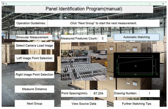
Figure 21.
Panel 1 recognition results.

Figure 22.
Panel 2 recognition results.
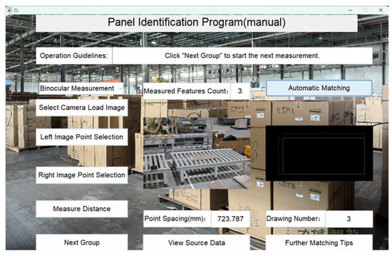
Figure 23.
Panel 3 recognition results.
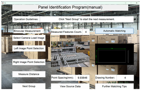
Figure 24.
Panel 4 recognition results.
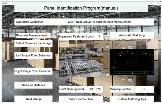
Figure 25.
Panel 5 recognition results.

Figure 26.
Panel 6 recognition results.

Figure 27.
Panel 7 recognition results.
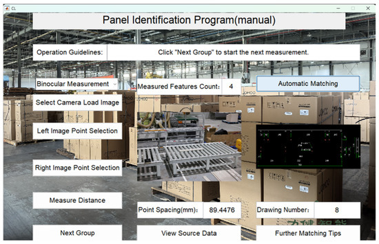
Figure 28.
Panel 8 recognition results.
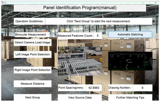
Figure 29.
Panel 9 recognition results.
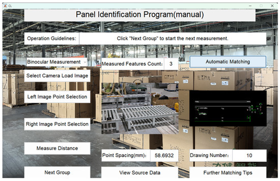
Figure 30.
Panel 10 recognition results.

Figure 31.
Panel 11 recognition results.
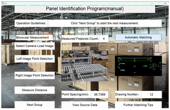
Figure 32.
Panel 12 recognition results.
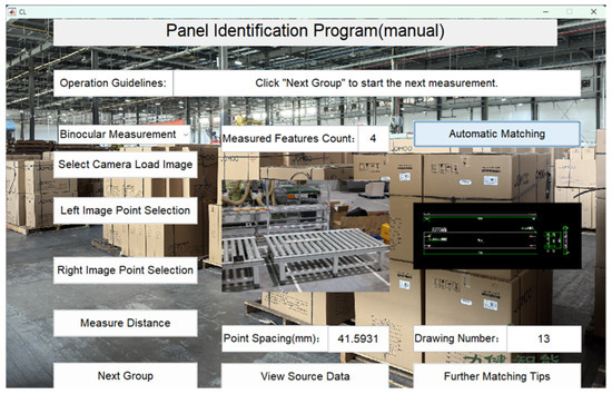
Figure 33.
Panel 13 recognition results.
5. Conclusions
This paper addresses the challenge of panel identity recognition in home decoration panel production lines by proposing a high-precision recognition method based on close-range photogrammetry. By combining panel size and hole position feature information, a label-free identity discrimination mechanism is established. Through practical validation, the system achieved a recognition accuracy of 100%, demonstrating excellent stability and adaptability in a real production environment with multiple panel models and no physical ID labels. This method has been deployed and tested on the JOMOO bathroom cabinet panel automation production line, validating its feasibility and engineering value in intelligent manufacturing scenarios. It provides technical support for achieving flexible and intelligent production in the home decoration industry.
Although the current system has achieved high recognition accuracy and the entire process has been automated, the system may still face some complex situations in specific environments. Continuous algorithm optimization is necessary to further enhance its stability and adaptability. In future work, the aim is to further enhance the intelligence of the image processing algorithms, achieving full-process automation from data acquisition to identity discrimination. This will further improve the system’s real-time performance, stability, and engineering adaptability.
Author Contributions
Conceptualization, E.L. and Z.G.; methodology, X.L.; software, X.L.; validation, Z.G., X.L.; formal analysis, E.L.; investigation, R.L.; resources, R.L.; data curation, X.L.; writing—original draft preparation, Z.G.; writing—review and editing, E.L.; visualization, Z.G.; supervision, D.Z.; project administration, D.Z.; funding acquisition, D.Z. and R.L. All authors have read and agreed to the published version of the manuscript.
Funding
Research on Calibration Method of Distributed Visual Perception System for Intelligent Agricultural Machinery Cluster in Hilly and Mountainous Areas: 2024AFB501; Digital Twin System for Industrialized Aquaculture Farming Systems: 2023010402010589.
Data Availability Statement
The data used to support the findings of this study are available from the corresponding author upon request.
Conflicts of Interest
The authors declare no conflicts of interest.
References
- Bono, F.M.; Radicioni, L.; Cinquemani, S. A Novel Approach for Quality Control of Automated Production Lines Working under Highly Inconsistent Conditions. Eng. Appl. Artif. Intell. 2023, 122, 106149. [Google Scholar] [CrossRef]
- Zhao, H.; Wan, F.; Lei, G.; Xiong, Y.; Xu, L.; Xu, C.; Zhou, W. LSD-YOLOv5: A Steel Strip Surface Defect Detection Algorithm Based on Lightweight Network and Enhanced Feature Fusion Mode. Sensors 2023, 23, 6558. [Google Scholar] [CrossRef]
- Horizral, L.; Rosová, A.; Ondov, M.; Šofranko, M. Redesign of the Manual Parcel Sorting Process in a Selected Company. Transp. Res. Procedia 2025, 87, 44–49. [Google Scholar] [CrossRef]
- Zhou, S.; Zhong, M.; Chai, X.; Zhang, N.; Zhang, Y.; Sun, Q.; Sun, T. Framework of Rod-like Crops Sorting Based on Multi-Object Oriented Detection and Analysis. Comput. Electron. Agric. 2024, 216, 108516. [Google Scholar] [CrossRef]
- Glučina, M.; Anđelić, N.; Lorencin, I.; Car, Z. Detection and Classification of Printed Circuit Boards Using YOLO Algorithm. Electronics 2023, 12, 667. [Google Scholar] [CrossRef]
- Luo, B. Integrating Multiple Attention Mechanism Fusion Based YOLO Logistics Sorting and Detection Model. In Proceedings of the 2025 8th International Conference on Advanced Algorithms and Control Engineering (ICAACE), Shanghai, China, 21–23 March 2025; pp. 1196–1201. [Google Scholar]
- Ge, W.; Chen, S.; Hu, H.; Zheng, T.; Fang, Z.; Zhang, C.; Yang, G. Detection and Localization Strategy Based on YOLO for Robot Sorting under Complex Lighting Conditions. Int. J. Intell. Robot. Appl. 2023, 7, 589–601. [Google Scholar] [CrossRef]
- Huo, J.; Shi, B.; Zhang, Y. An Object Detection Method for the Work of an Unmanned Sweeper in a Noisy Environment on an Improved YOLO Algorithm—Signal, Image and Video Processing. Signal Image Video Process. 2023, 17, 4219–4227. [Google Scholar] [CrossRef]
- Shen, L.; Li, X.; Yang, W.; Wang, Q. Tlb-yolo: A Rapid and Efcient Real-time Algorithm for Box-Type Classification and Barcode Recognition on the Moving Conveying and Sorting Systems; Springer Science and Business Media LLC: Berlin/Heidelberg, Germany, 2024. [Google Scholar] [CrossRef]
- Nocerino, E.; Menna, F.; Verhoeven, G.J. Good vibrations? How image stabilisation influences photogrammetry. Int. Arch. Photogramm. Remote Sens. Spat. Inf. Sci. 2022, 46, 395–400. [Google Scholar] [CrossRef]
- Yuan, F.; Xia, Z.; Tang, B.; Yin, Z.; Shao, X.; He, X. Calibration Accuracy Evaluation Method for Multi-Camera Measurement Systems. Measurement 2025, 242, 116311. [Google Scholar] [CrossRef]
- Jiang, S.; Jiang, H.; Ma, S.; Jiang, Z. Detection of Parking Slots Based on Mask R-CNN. Appl. Sci. 2020, 10, 4295. [Google Scholar] [CrossRef]
- Tao, W.; Hua, X.; Yu, K.; Wang, R.; He, X. A Comparative Study of Weighting Methods for Local Reference Frame. Appl. Sci. 2020, 10, 3223. [Google Scholar] [CrossRef]
- Wolf, P.R.; DeWitt, B.A. Elements of Photogrammetry: With Applications in GIS, 3rd ed.; McGraw Hill: Columbus, OH, USA, 2000. [Google Scholar]
- Ballard, D.H. Generalizing the Hough Transform to Detect Arbitrary Shapes. Pattern Recognit. 1981, 13, 111–122. [Google Scholar] [CrossRef]
- Hassanein, A.S.; Mohammad, S.; Sameer, M.; Ragab, M.E. A Survey on Hough Transform, Theory, Techniques and Applications. arXiv 2015, arXiv:1502.02160. [Google Scholar] [CrossRef]
- James, M.R.; Robson, S. (PDF) Straightforward Reconstruction of 3D Surfaces and Topography with a Camera: Accuracy and Geoscience Application. J. Geophys. Res. Earth Surf. 2012, 117. [Google Scholar] [CrossRef]
- Chen, Y.; Jin, X.; Dai, Q. Distance Measurement Based on Light Field Geometry and Ray Tracing. Opt. Express 2017, 25, 59–76. [Google Scholar] [CrossRef]
- Ji, Q.; Costa, M.S.; Haralick, R.M.; Shapiro, L.G. A Robust Linear Least-Squares Estimation of Camera Exterior Orientation Using Multiple Geometric Features. ISPRS J. Photogramm. Remote Sens. 2000, 55, 75–93. [Google Scholar] [CrossRef]
- Zhuang, S.; Zhao, Z.; Cao, L.; Wang, D.; Fu, C.; Du, K. A Robust and Fast Method to the Perspective-n-Point Problem for Camera Pose Estimation. IEEE Sens. J. 2023, 23, 11892–11906. [Google Scholar] [CrossRef]
- Grussenmeyer, P.; Khalil, O.A. Solutions for Exterior Orientation in Photogrammetry: A Review. Photogramm. Rec. 2002, 17, 615–634. [Google Scholar] [CrossRef]
- Zhao, W.; Su, X.; Chen, W. Whole-Field High Precision Point to Point Calibration Method. Opt. Lasers Eng. 2018, 111, 71–79. [Google Scholar] [CrossRef]
- Dahnert, M.; Hou, J.; Niessner, M.; Dai, A. Panoptic 3D Scene Reconstruction from a Single RGB Image. In Advances in Neural Information Processing Systems; Curran Associates, Inc.: Morehouse, NY, USA, 2021; Volume 34, pp. 8282–8293. [Google Scholar]
- Lu, E.; Liu, Y.; Zhao, Z.; Liu, Y.; Zhang, C. A Weighting Radius Prediction Iteration Optimization Algorithm Used in Photogrammetry for Rotary Body Structure of Port Hoisting Machinery. IEEE Access 2021, 9, 140397–140412. [Google Scholar] [CrossRef]
- Lu, E. Multi-LineIntersection Photogrammetric Method and Its Application in Port Machinery. Ph.D. Dissertation, Wuhan University of Technology, Wuhan, China, 2022. [Google Scholar]
- Mitishita, E.A.; Santos de Salles Graça, N.L. The Influence of Redundant Images in Uav Photogrammetry Application. In Proceedings of the IGARSS 2018–2018 IEEE International Geoscience and Remote Sensing Symposium, Valencia, Spain, 22–27 July 2018; pp. 7894–7897. [Google Scholar]
- Ricolfe-Viala, C.; Sánchez-Salmerón, A.-J. Correcting Non-Linear Lens Distortion in Cameras without Using a Model. Opt. Laser Technol. 2010, 42, 628–639. [Google Scholar] [CrossRef]
- Ricolfe-Viala, C.; Sanchez-Salmeron, A.-J. Lens Distortion Models Evaluation. Appl. Opt. 2010, 49, 5914–5928. [Google Scholar] [CrossRef]
- Lai, S.; Cheng, Z.; Zhang, W.; Chen, M. Wide-Angle Image Distortion Correction and Embedded Stitching System Design Based on Swin Transformer. Appl. Sci. 2025, 15, 7714. [Google Scholar] [CrossRef]
Disclaimer/Publisher’s Note: The statements, opinions and data contained in all publications are solely those of the individual author(s) and contributor(s) and not of MDPI and/or the editor(s). MDPI and/or the editor(s) disclaim responsibility for any injury to people or property resulting from any ideas, methods, instructions or products referred to in the content. |
© 2025 by the authors. Licensee MDPI, Basel, Switzerland. This article is an open access article distributed under the terms and conditions of the Creative Commons Attribution (CC BY) license (https://creativecommons.org/licenses/by/4.0/).