FLOW-GLIDE: Global–Local Interleaved Dynamics Estimator for Flow Field Prediction

Abstract

Accurate prediction of the flow field is crucial to evaluating the aerodynamic performance of an aircraft. While traditional computational fluid dynamics (CFD) methods solve the governing equations to capture both global flow structures and localized gradients, they are computationally intensive. Deep learning-based surrogate models offer a promising alternative, yet often struggle to simultaneously model long-range dependencies and near-wall flow gradients with sufficient fidelity. To address this challenge, this paper introduces the Message-passing And Global-attention block (MAG-BLOCK), a graph neural network module that combines local message passing with global self-attention mechanisms to jointly learn fine-scale features and large-scale flow patterns. Building on MAG-BLOCK, we propose FLOW-GLIDE, a cross-architecture deep learning framework that learns a mapping from initial conditions to steady-state flow fields in a latent space. Evaluated on the AirfRANS dataset, FLOW-GLIDE outperforms existing models on key performance metrics. Specifically, it reduces the error in the volumetric flow field by 62% and surface pressure prediction by 82% compared to the state-of-the-art.

1. Introduction

In the field of aerospace engineering, accurate flow field prediction plays a pivotal role in the design, analysis, and control of high-performance systems such as aircraft, launch vehicles, and reentry capsules. Traditional computational fluid dynamics (CFD) methods, although highly accurate, often involve solving complex partial differential equations (PDEs) on fine-resolution meshes, leading to prohibitively expensive computations, particularly for high-fidelity simulations. These limitations pose significant challenges for rapid design iteration, making decisions in real time, and quantifying uncertainty. As a result, there is a growing demand for efficient surrogate models capable of predicting flow fields with reduced computational overhead while maintaining physical accuracy. In recent years, neural network-based approaches have emerged as a promising alternative, offering fast and scalable solutions for modeling nonlinear flow dynamics across diverse geometries and conditions.

Various network models in deep learning are applied to flow field modeling, such as Convolution Neural Network (CNN) [1,2,3,4,5,6,7] and Graph Neural Network (GNN) [8,9,10,11,12,13,14]. Yu et al. used a knowledge-enhanced end-to-end CNN as the core, and replaced the high-cost numerical calculation of unsteady flow around blunt bodies with near-real-time pixel-to-pixel prediction through wind engineering priors such as non-uniform encryption and transfer learning [15]. Lee et al. used CNNs with four progressive resolutions and physical conservation constraints to achieve fast prediction of three-dimensional cylindrical wakes [16]. Du et al. builds an integrated CNN-based pipeline that unifies airfoil parameterization, flow prediction, and rapid inverse design [17]. Pfaff et al. proposed MeshGraphNet, which combines multi-space message passing with a learnable adaptive re-meshing mechanism [18]. Li et al. achieved fast and high-precision prediction of two-dimensional unsteady incompressible flows on unstructured grids by embedding finite volume constraints into losses and combining two-level message aggregation with spatial integration layers, significantly suppressing error accumulation and accelerating training and inference [19]. Zou et al. combine finite difference residual with graph to make a differentiable GC-FDM. Combined with block-level coordinate transformation and unit-enhanced message passing, it realizes label-free, physically constrained flow field solution on multi-block conforming grids [20].

In order to enhance the global feature learning capabilities of CNN and GNN, the researchers made some adjustments to the network architecture. Zhang et al. fused the signed distance function matrix and multichannel features based on the U-Net architecture, and used independent decoders for each physical quantity, which greatly improved the accuracy of multi-shape flow field prediction [21]. Chen et al. proposed a U-Net network model based on coordinate transformation encoding to quickly and accurately infer the flow of two-dimensional compressible flow fields on different wing sections [22]. In addition, Chen et al. also combined the attention mechanism with the U-Net architecture to quickly and accurately predict transonic unsteady airfoil flows [23]. Fortunato et al. introduced Multiscale MeshgraphNets based on Pfaff [18] for multiscale feature [24]. Gao et al. borrowed the U-Net architecture and proposed the graph U-Net containing graph pooling and graph convolution for global and local feature [25].

The Transformer architecture [26] has gained prominence due to its exceptional natural language processing capabilities [27,28,29]. Based on this architecture and its core component attention mechanism, Wu et al. used learnable physical slices and Physics-Attention to transfer the multi-head attention of Transformer from massive grid points to physical tokens, achieving high-precision, linear-time solution of PDE in arbitrarily complex geometric domains [30]. Luo et al. extended Transolver, enables the first success in accurately solving PDEs discretized on million-scale geometries [31]. Zhou et al. utilize complete PDE component and decoupled conditional Transformer to explicitly inject equation knowledge into the network, achieving strong generalization and state-of-the-art (SOTA) performance under multiple data sets, multiple equations, and multiple boundary conditions [32]. Xiao et al. combined geometric attention with implicit neural fields, and efficiently encoded the geometric information of irregular point clouds [33]. Alki et al. proposed a unified neural operator framework that does not rely on a specific grid or particle structure [34].

CNNs and GNNs can effectively capture local flow structure, but they struggle with global interactions. CNNs require rasterization/pixelization of the computational mesh [35], which introduces aliasing and geometric-edge distortion. Moreover, both CNNs and standard GNNs are inherently local operators whose receptive fields expand only with depth, leading to limited effective context [36,37]. Deepening GNNs to extend their reach typically induces feature over-smoothing [38], whereas architectural workarounds that exchange information at distance can distort the original graph representation. While attention mechanisms excel at modeling long-range dependencies, vanilla attention lacks an explicit inductive bias for grid locality and non-uniform node density. The resulting global aggregation tends to dilute small-scale structure and makes it difficult to prioritize key node-dense regions such as the boundary layer and wake flow. Ultimately, native attention struggles to simultaneously preserve strong local variations near walls and capture global coupling. This limitation requires the incorporation of local priors or grid-aware mechanisms. Collectively, these limitations hinder a robust balance between local detail and global coupling when both must be learned simultaneously.

Based on this, we propose a novel Global–Local learning module, which utilizes the spatial information in the Mesh-Based representation. The Global–Local learning module uses GNN and attention mechanism to extract local features and global features based on the mesh, and fuses features of different scales. Stacking the Global–Local learning module to build Global–Local Interleaved Dynamics Estimator(FLOW-GLIDE), which balances the learning process of features of different scales, significantly improving the prediction accuracy of dense mesh areas and areas with large physical space spans. The main contributions of this study can be summarized as follows:

• This paper introduces a multiscale feature learning module, a novel Global–Local feature learning method that can effectively balance the learning process of different features of the neural network without the need for auxiliary learning methods.
• Based on the novel feature learning method, we propose FLOW-GLIDE, which can learn from mesh-based geometric representations and significantly improve the prediction accuracy in obstacle boundary layers and wake regions.
• A series of experiments were conducted on a data set based on aircraft airfoils to verify the effectiveness of the proposed model. Quantitative comparisons with other baseline models were additionally performed. The experimental results show that our model significantly improves prediction accuracy compared to single-type network models and other multi-scale feature fusion models.

This paper is summarized as follows: Section 2 defines the main research questions of this paper and describes the MAG-BLOCK and FLOW-GLIDE in detail. Comparison of the results with the ground truth and conduct quantitative analysis with the baseline model in Section 3. Finally, the conclusion is presented in Section 4.

2. Methodology

2.1. Problem Setup

This work addresses learning the mapping from initial conditions to incompressible steady high–Reynolds number flow over an 2D airfoil, which can be shown as follows:

$$\begin{array}{c}\hfill F_{\theta }:(\mathrm{geometry},\mathrm{operating}\mathrm{conditions})\mapsto {(u_x,u_y,p,{\nu }_t)}_{\mathrm{steady}}\end{array}$$

(1)

In incompressible high-Reynolds condition, flow are governed by Reynolds-Averaged Navier–Stokes (RANS) equations as follows:

$$\begin{array}{c}\hfill \begin{array}{cc}\hfill {\partial }_i{\overline{u}}_i& =0\hfill \\ \hfill {\partial }_j\left({\overline{u}}_i{\overline{u}}_j\right)& =-{\partial }_i\left({\displaystyle \frac{\overline{p}}{\rho }}\right)+(\nu +{\nu }_t){\partial }_{jj}^2{\overline{u}}_i,i\in \{1,2\}\hfill \end{array}\end{array}$$

(2)

where $\overline{·}$ presents an ensemble-averaged quantity, ${\partial }_i$ the partial derivative with respect to the $i$ spatial components. u, p, $\rho$ are fluid velocity, pressure and the fluid mass. $\nu$ and ${\nu }_t$ are the fluid kinematic viscosity and the fluid kinematic turbulent viscosity respectively.

At high Reynolds number, the surface flow exhibits thin, high-shear boundary layers, separation and vortex shedding, together with long-range coupling from the boundary layer into the downstream wake flow. Our model focuses on learning local features of the airfoil surface as well as global features of the entire flow field, including the wake evolving from the surface.

In order to better describe the method proposed in this paper, the symbols in

Table 1. Definition of main symbols.

Symbol	Definition
$\mathcal{V}$	Point sets
$V_a$	Point a
$\mathcal{E}$	Edge sets
$E_{ab}$	Edge that connect point a and b
N	The number of total points
$\mathrm{\Omega }$	The entire flow field
$\mathcal{G}$	The input graph structure
$n_a$	Initial feature of point a
$e_{ab}$	Initial feature of edge ab
$d_a$	The number of a domain’s dimensions
${\mathbf{n}}_a^l$	Latent feature of point a after l-layer Network
${\mathbf{e}}_{ab}^l$	Latent feature of edge ab after l-layer Network
$\psi$	Multilayer perceptron(MLP)
g	Message Passing layer
A	Attention layer

will be used.

2.2. Global–Local Interleaved Dynamics Estimator

In this section, we introduce the overall architecture of our network model, which is called FLOW-GLIDE, and how it learns the flow field distribution from the features of the sampled points.

FLOW-GLIDE learns pairwise and higher-order relationships among mesh points to capture both local variations and domain-level trends in the flow field. The architecture interleaves Message Passing layers with attention layers, providing complementary inductive biases: the former resolves neighborhood-scale structures, such as near-wall and wake interactions, while the latter models long-range couplings across the domain. This alternation yields a balanced latent representation that does not privilege any single feature scale.

As shown in Figure 1, Given a two-dimensional geometry and its discrete points on the original mesh in AirfRANS [39], let the continuous domain be $\mathrm{\Omega }\subset {\mathbb{R}}^2$, and the original discrete domain be ${\mathcal{V}}_{origin}={\left\{V_i\right\}}_{i=1}^N$ and ${\mathcal{E}}_{origin}={\left\{E_{ij}=(V_i,V_j)\right\}}_{i=1,j=2,i\ne j}^{N,N}$. To reduce computational complexity and preserve the local structure, as well as compare to the baseline model, structure-preserving subsampling strategy is applied under the premise of geometric consistency, obtaining a node set $\mathcal{V}=\{V_1,\dots ,V_n\}(n\ll N)$ and a edge set $\mathcal{E}=\{E_{12},\dots ,E_{ij}\}(i\ll N,j\ll N)$. The sampling strategy consists of two steps: First, 2000 points are randomly sampled from the entire discrete point set ${\mathcal{V}}_{origin}$; then, using the K-hop algorithm with k = 5, a second step of sampling is simultaneously performed and connecting along the original grid lines to get $\mathcal{V}$ and $\mathcal{E}$.

Based on this, an undirected graph $\mathcal{G}=(\mathcal{V},\mathcal{E})$ is constructed. For each node, the initial features $n_i\in {\mathbb{R}}^{d_{\mathrm{in}}^v}$ comprise global coordinate $po{s}_x$ and $po{s}_y$, inlet velocity $V_{inflow}^x$ and $V_{inflow}^y$, the distance from points to airfoil surface d, the components of the normal vector in the x and y directions $norma{l}_x$ and $norma{l}_y$. Specifically, if the point is in flow field, then the zero vector is set. The initial feature of each edge $e_{ij}\in {\mathbb{R}}^{d_{\mathrm{in}}^e}$ is the difference between the features of the points at its two ends, except for the coordinates.

After subsampling, the node features and edge features will be projected into the latent space $D\subset {\mathbb{R}}^{d_{hidden}}$ through MLP, as shown in Equation (3):

$$\begin{array}{c}\hfill {\mathbf{n}}_i^0={\psi }_n\left(n_i\right)\\ \hfill {\mathbf{e}}_{ij}^0={\psi }_e\left(e_{ij}\right)\end{array}$$

(3)

where, ${\mathbf{n}}_i^0$ and ${\mathbf{e}}_{ij}^0$ represent the node and edge feature respectively in the latent space. The $\psi (·)$ reject the MLP.

To emphasize the local structure, FLOW-GLIDE begins with graph module. After an encoder projects node attributes into the latent space, the undirected graph $\mathcal{G}$ is processed by three Message Passing layers, which utilized FVGN [19]. This configuration enabling aggregation of informative neighborhood interactions while remaining sufficiently shallow to mitigate feature oversmoothing of node representations. After Message Passing layers, the latent feature ${\mathbf{n}}_i^0$ and ${\mathbf{e}}_{ij}^0$ aggregate the neighbor node information to ${\mathbf{n}}_i^L$ and ${\mathbf{e}}_{ij}^L$. Local feature extraction can be described as follows:

$$\begin{array}{c}\hfill {\mathbf{n}}_i^L=g^L\left(g^{L-1}(\dots g^l(\dots g^1\left({\mathbf{n}}_i^0\right)))\right),1\le l\le L\\ \hfill {\mathbf{e}}_{ij}^L=g^L\left(g^{L-1}(\dots g^l(\dots g^1\left({\mathbf{e}}_{ij}^0\right)))\right),1\le l\le L\end{array}$$

(4)

where g represents the Message Passing layer. $L=3$ is determined as the subsequent experimental setup.

After local feature extraction, the undirected graph $\mathcal{G}$ is passed to a global attention module, where Transolver [30] is employed as the attention layer. $\mathcal{G}$ will be decomposed into a set of learnable slices $\mathbf{s}={\left\{{\mathbf{s}}_k\right\}}_{k=1}^M$. Each slice is then compressed into a physics-aware token by aggregating node embeddings together with spatially weight. A multi-head cross-attention operator subsequently evaluates the contribution of each token to each output, assigning token-specific attention weights and thereby modeling long-range couplings across the domain. Global feature extraction can be described as follows:

$$\begin{array}{c}\hfill {\mathbf{n}}_i^{2L}=A^L\left(A^{L-1}(\dots A^l(\dots A^1\left({\mathbf{n}}_i^L\right)))\right),1\le l\le L\end{array}$$

(5)

where A represent the attention layer. Only pass node features are passed to attention layer, as shown in Equation (5). $L=1$ attention layer is employed in subsequent experimental setup.

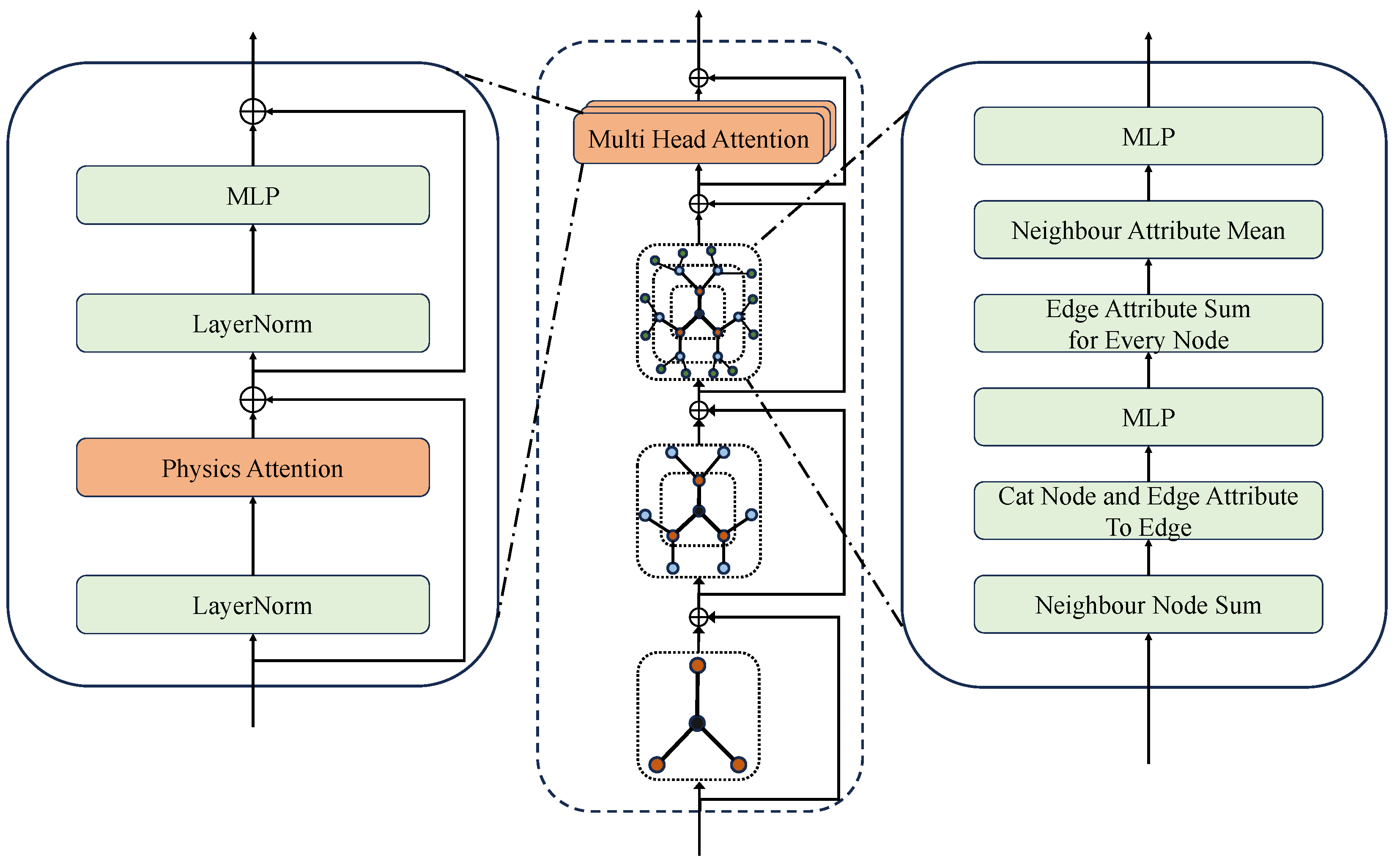
Building on the components above, the principal module, MAG-BLOCK, is constructed, coupling three Message Passing layers with an attention layer through residual projections. Stacking MAG-BLOCKs yields a deep architecture with alternating local–global stages, progressively enriching neighborhood-scale features and domain-wide dependencies without privileging any single scale. The constituent layers are described in detail in Section 2.2.

After stacking B instances of MAG-BLOCK, the model produces node-level latent embeddings that jointly encode local structure and long-range couplings. A decoder architecturally symmetric to the encoder then maps these embeddings to pointwise predictions of the target flow variables, yielding the full flow-field distribution, which can be shown as Equation (6).

$$\begin{array}{c}\hfill n_i^{pred}={\psi }_{\mathrm{dec}}\left({\mathbf{n}}_i^K\right)\end{array}$$

(6)

2.3. Global–Local Learning Module

The structure of Global–Local learning module is shown in Figure 2, which is called MAG-BLOCK. After each Message Passing layer and attention layer, there is a residual connection layer to maintain training stability. The right side of Figure 2 shows the calculation process of the Message Passing layer, and the left side shows the calculation process of the attention mechanism. We now describe the learning procedure within MAG-BLOCK in detail. Figure 2 presents the architecture of the Global–Local learning module, MAG-BLOCK. Each message-passing and attention layer is wrapped with a residual connection to promote training stability. The right panel of Figure 2 details the computations in the Message Passing layer, whereas the left panel illustrates the attention mechanism. Next, the learning procedure within MAG-BLOCK is detailed.

Let $\mathcal{G}=(\mathcal{V},\mathcal{E})$ be the undirected graph, with node features ${\mathbf{n}}_i\in {\mathbb{R}}^{d_{hidden}}$ and edge features ${\mathbf{e}}_{ij}\in {\mathbb{R}}^{d_{hidden}}$. Denote the 1-hop neighborhood of node i by $\mathcal{N}\left(i\right)$. For the endpoints i and j of each edge $E_{ij}$, calculate the sum of the features of adjacent nodes ${\tilde{\mathbf{n}}}_i$ and ${\tilde{\mathbf{n}}}_j$, respectively:

$${\tilde{\mathbf{n}}}_i=\sum _{m\in \mathcal{N}\left(i\right)}{\mathbf{n}}_m^l,{\tilde{\mathbf{n}}}_j=\sum _{p\in \mathcal{N}\left(j\right)}{\mathbf{n}}_p^l.$$

(7)

Then concatenate these descriptors with the current edge attribute in the fixed order $[{\tilde{\mathbf{n}}}_i\Vert {\tilde{\mathbf{n}}}_j\Vert {\mathbf{e}}_{ij}]$ and pass the result through an MLP ${\psi }_{\mathrm{edge}}$ for edge to obtain the updated edge feature:

$${\mathbf{e}}_{ij}^{l+1}={\psi }_{\mathrm{edge}}\left([{\tilde{\mathbf{n}}}_i\Vert {\tilde{\mathbf{n}}}_j\Vert {\mathbf{e}}_{ij}^l]\right).$$

(8)

where $(·)\Vert (·)$ is concatenation.

With the updated edge features ${\mathbf{e}}_{ij}^{l+1}$ obtained from the edge stage, the aggregation of information to each points $V_i$ is performed in two steps. The first step computes an incident edge feature sum, which aggregates the messages incoming to point $V_i$:

$${\tilde{\mathbf{e}}}_i=\sum _{j\in \mathcal{N}\left(i\right)}{\mathbf{e}}_{ij}^{l+1}.$$

(9)

where ${\tilde{\mathbf{e}}}_i$ refers to the sum of the attributes of all edges connected to point $V_i$.

Equal weighting is then applied to all ${\tilde{\mathbf{e}}}_j$ of neighboring points of point $V_i$, yielding a mean of features ${\overline{\mathbf{n}}}_i$ on point $V_i$:

$${\overline{\mathbf{n}}}_i={\displaystyle \frac{1}{\left|\mathcal{N}\right(i\left)\right|}}\sum _{j\in \mathcal{N}\left(i\right)}{\tilde{\mathbf{e}}}_j.$$

(10)

${\overline{\mathbf{n}}}_i$ is concatenated with the current node feature ${\mathbf{n}}_i^l$ and passed through an MLP ${\psi }_{node}$ for node to produce the updated node attribute:

$${\mathbf{n}}_i^{l+1}={\psi }_{node}\left([{\overline{\mathbf{n}}}_i\Vert {\mathbf{n}}_i^l]\right)$$

(11)

After three message-passing layers, Transolver [30] is employed as the global feature learning module. Prior to global aggregation, the node feature ${\mathbf{n}}_i^l$ are normalized with LayerNorm. With H head attention, a linear projection $f_{\mathrm{weight}}$ and a Softmax layer yields M slice weights $\mathbf{w}={\left\{{\mathbf{w}}_{i,k}^h\right\}}_{i=1,k=1}^{N,M}$ for each head h:

$${\left\{{\mathbf{w}}_{i,k}^h\right\}}_{i=1,k=1}^{N,M}={\left\{\mathrm{Softmax}\left(f_{weight}\left({\mathbf{n}}_i^l\right)\right)\right\}}_{i=1}^N$$

(12)

For slice k, a physics-aware token ${\mathbf{t}}_k^h$ is produced by weighted reduction of node embeddings according to Equation (13):

$${\mathbf{t}}_k^h={\displaystyle \frac{{\sum }_{i=1}^N{\mathbf{w}}_{i,k}^h{\mathbf{s}}_i^h}{{\sum }_{i=1}^N{\mathbf{w}}_{i,k}^h}},k=(1,\dots ,M)h=(1,\dots ,H)$$

(13)

Each token ${\mathbf{t}}_k^h$ is input into multi-head attention. For head h with head dimension $d_h$ generates its own query ${\mathbf{Q}}_k^h$, key ${\mathbf{K}}_k^h$, and value ${\mathbf{V}}_k^h$ vectors for each token through a linear layer. The attention weights encoding token-to-token correlations and outputs are

$$\begin{array}{c}\hfill {\mathbf{A}}_k^h=\mathrm{Softmax}\left({\displaystyle \frac{{\mathbf{Q}}_k^h{\left({\mathbf{K}}_k^h\right)}^{\top }}{\sqrt{d_h}}}\right)\\ \hfill {\mathbf{z}}_k^h={\mathbf{A}}_k^h{\mathbf{V}}_k^h.\end{array}$$

(14)

Afterward, learned tokens ${\mathbf{z}}_k^h$ recomposes to nodes attribute with slice weights on each head, then compose attribute go through a linear layer to obtain the attention outputs:

$$\begin{array}{c}\hfill {\mathbf{n}}_i^h=\sum _{k=1}^M{\mathbf{w}}_{i,k}^h{\mathbf{z}}_k^h,\\ \hfill {\tilde{\mathbf{n}}}_i=f\left({\mathbf{n}}_i^h\right)\end{array}$$

(15)

where f is a linear projection. ${\tilde{\mathbf{n}}}_i$ will also go through a LayerNorm and an MLP, and get the final output after the residual connection. The entire learning process can be expressed as follows:

$$\begin{array}{c}\hfill {\mathbf{n}}_i^{\prime }={\mathbf{n}}_i^l+\mathrm{Attention}\left(\mathrm{LN}\left({\mathbf{n}}_i^l\right)\right),\\ \hfill {\mathbf{n}}_i^{l+1}={\mathbf{n}}_i^{\prime }+{\psi }_{attn}\left(\mathrm{LN}\left({\mathbf{n}}_i^{\prime }\right)\right).\end{array}$$

(16)

where $\mathrm{LN}$ represents layernorm and $\mathrm{Attention}$ contains learning routine from Equation (14) to Equation (16).

2.4. Loss Function

$${\mathcal{L}}_{vol}={\displaystyle \frac{\sqrt{{\sum }_{i=1}^N{(y_i^{pred}-y_i)}^2}}{\sqrt{{\sum }_{i=1}^N{y}_i^2}}}$$

(17)

$${\mathcal{L}}_{surf}={\displaystyle \frac{\sqrt{{\sum }_{i=1}^N{(p_i^{pred}-p_i)}^2}}{\sqrt{{\sum }_{i=1}^N{p}_i^2}}}$$

(18)

$$\mathcal{L}={\mathcal{L}}_{surf}+{\mathcal{L}}_{vol}$$

(19)

Relative $L_2$ error is used as the loss function. For volume nodes, the loss is evaluated jointly over all predicted variables—velocity components $v_x$ and $v_y$, pressure p, and turbulent viscosity ${\nu }_t$. For airfoil surface nodes, since only the reduced pressure is given, so the loss is restricted to the pressure channel. The final training objective is minimize the sum of the volumetric and surface relative $L_2$ terms.

3. Results and Discussion

3.1. Benchmark and Configures

AirfRANS [39] is used as the benchmark dataset, comprising 1000 two-dimensional steady incompressible RANS simulations of NACA 4- and 5-digit airfoils, with angles of attack ranging from −5° to 15° and Reynolds numbers between $2\times {10}^6$ and $6\times {10}^6$. For each case, a C-grid multi-block hexahedral mesh is generated using blockMesh in OpenFOAM v2112. Solutions are computed with simpleFOAM using the SIMPLEC algorithm and the SST turbulence model, and are advanced to convergence of drag and lift coefficients. The dataset provides four evaluation tasks, which are Full data regime, Scarce data regime, Reynolds extrapolation regime, and Angle of Attack (AoA) extrapolation. The results are reported on the full-regime, Reynolds-extrapolation, and AoA-extrapolation tracks, with comparisons made against baselines.

The baseline models used in AirfRANS include MLP, Graph U-Net [25], GraphSAGE [40], and PointNet [41]. For visualization comparison with FLOW-GLIDE, we additionally re-implement FVGN [19], MeshGraphNet [18], Transolver [30], together with MLP and GraphSAGE [40]. All these models were trained for 600 epochs using an initial learning rate of 0.001 and the ADAM optimizer with a latent space of feature length 128. The relative L2 loss function was used. In one MAG-BLOCK, three Message Passing layers and one attention layer are used. Additional comparisons are conducted with newer models, including GNO [42], GNOT [43], GINO [44], and Galerkin [45]. All experiments were conducted on an RTX 4090 GPU and the code was implemented using the PyTorch framework.

3.2. Comparison of Flow Fields

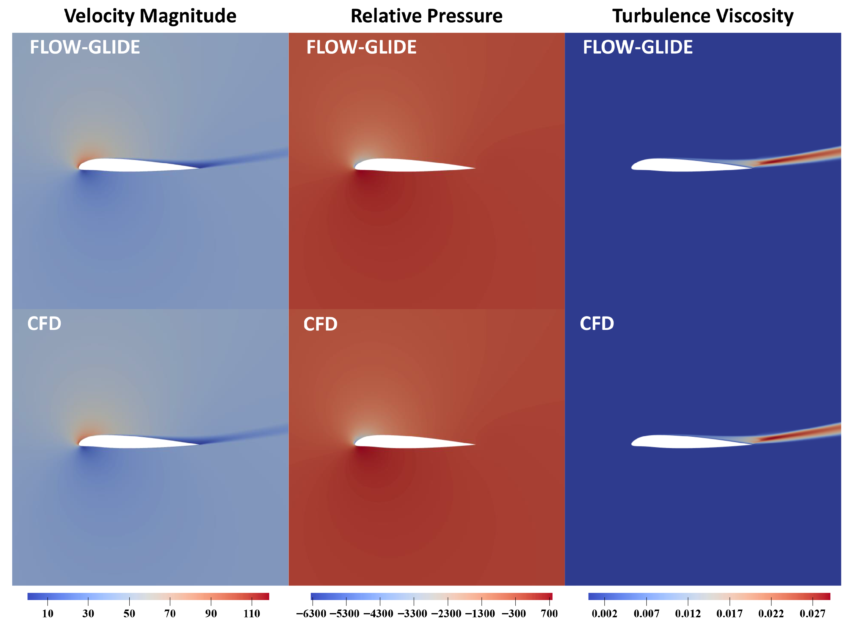
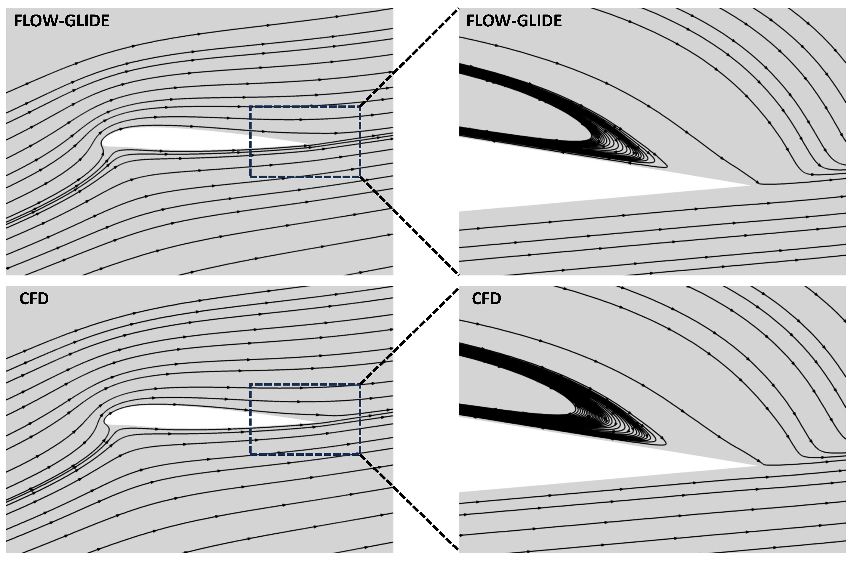
We compared the prediction results with CFD. Figure 3 and Figure 4 show the values of flow field variables and the distribution of streamlines when the angle of attack is 14.642° and the velocity is 39.741 m/s.

Figure 3 shows that FLOW-GLIDE reproduces the spatial organization of the two-dimensional flow with high fidelity. Locally, the leading-edge stagnation region and the near-wall acceleration along the suction side agree closely with the CFD reference. Globally, the growth of the boundary layer and the downstream development of the wake are consistently reproduced.

Figure 4 compares the predicted streamlines of FLOW-GLIDE with the CFD reference for the same operating condition. The left panels show the full field. The incoming flow decelerates to a leading-edge stagnation point, accelerates along the suction side, and recovers toward the trailing edge. The wake centerline orientation and the spacing of farfield streamlines are consistent between prediction and CFD, indicating that the global flow organization is faithfully reproduced.

The right panels magnify the boxed region near the trailing edge and highlight the recirculation bubble. FLOW-GLIDE resolves the family of closed streamlines inside the bubble and closely matches the CFD in the curvature of the outer shear layer that bounds the bubble, and the reattachment location where the shear layer impinges on the surface. The extent and height of the bubble are comparable to the reference, and no spurious secondary eddies are observed.

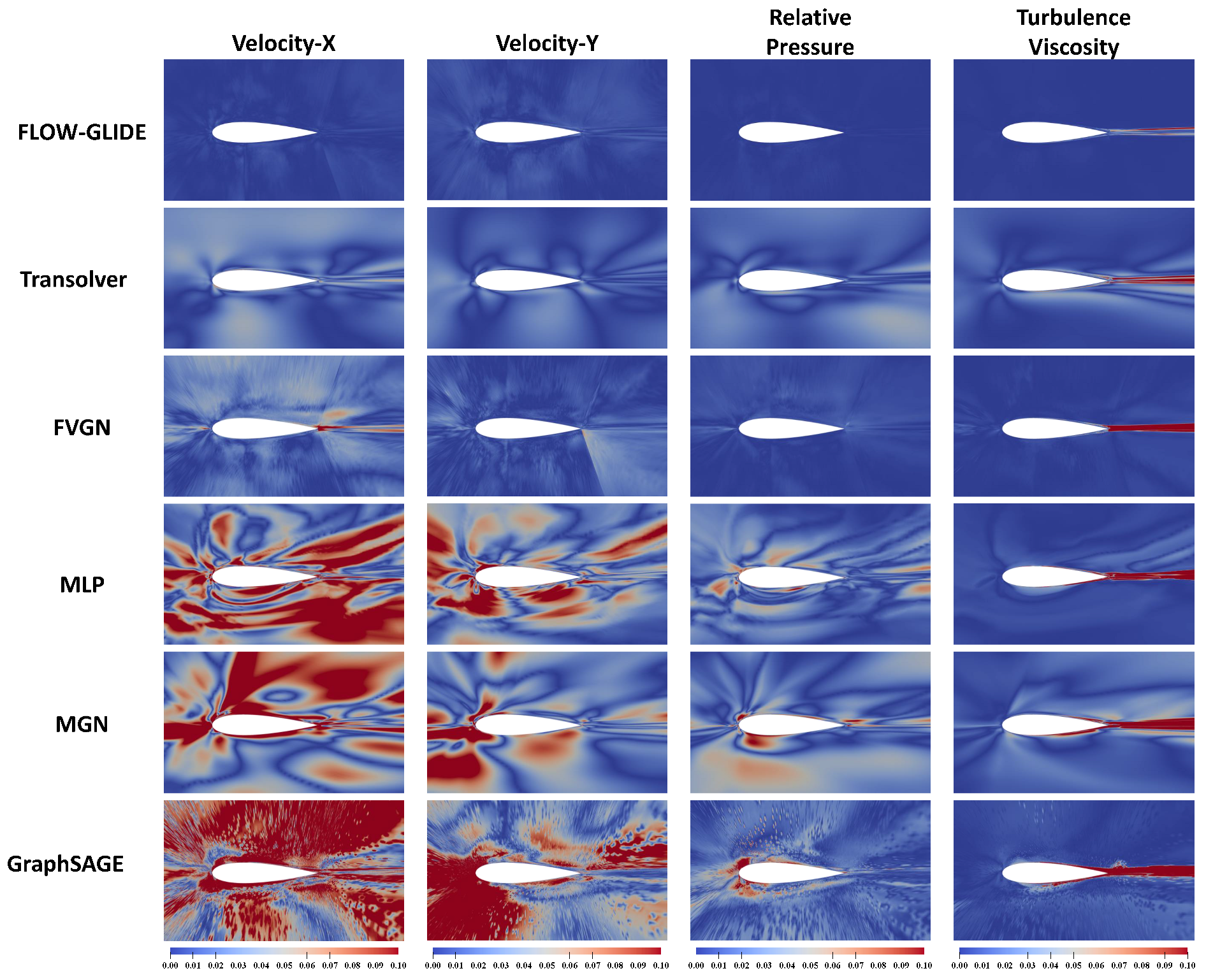
In addition to qualitative comparisons with the CFD fields, error visualizations are provided for the baseline models described in Section 3.1. Since differences in raw predictions are often visually indistinguishable under standard color mappings, pointwise relative $L_2$ errors are reported against the CFD reference fields to provide a more sensitive evaluation. Figure 5 reports the error across all predicted variables. To enable fair side-by-side comparison, all panels for a given variable use an identical color scale in the range $[0,{10}^{-1}]$. Lower values indicate better agreement.

FLOW-GLIDE attains the lowest errors for all components. Spatially, errors for all methods concentrate in the trailing-edge shear layer and wake, whereas the far field and most of the external flow remain below 0.01 for FLOW-GLIDE. The leading and trailing edge neighborhoods exhibit noticeably higher errors for the baselines, reflecting reduced accuracy in resolving local flow features. Although Transolver [30] is the SOTA model, its error maps still display residual bands of elevated wake error and localized hot spots near the leading edge, both attenuated in FLOW-GLIDE. Overall, the alternating local-then-global design reduces wake-core and near-edge errors without inflating far-field artifacts.

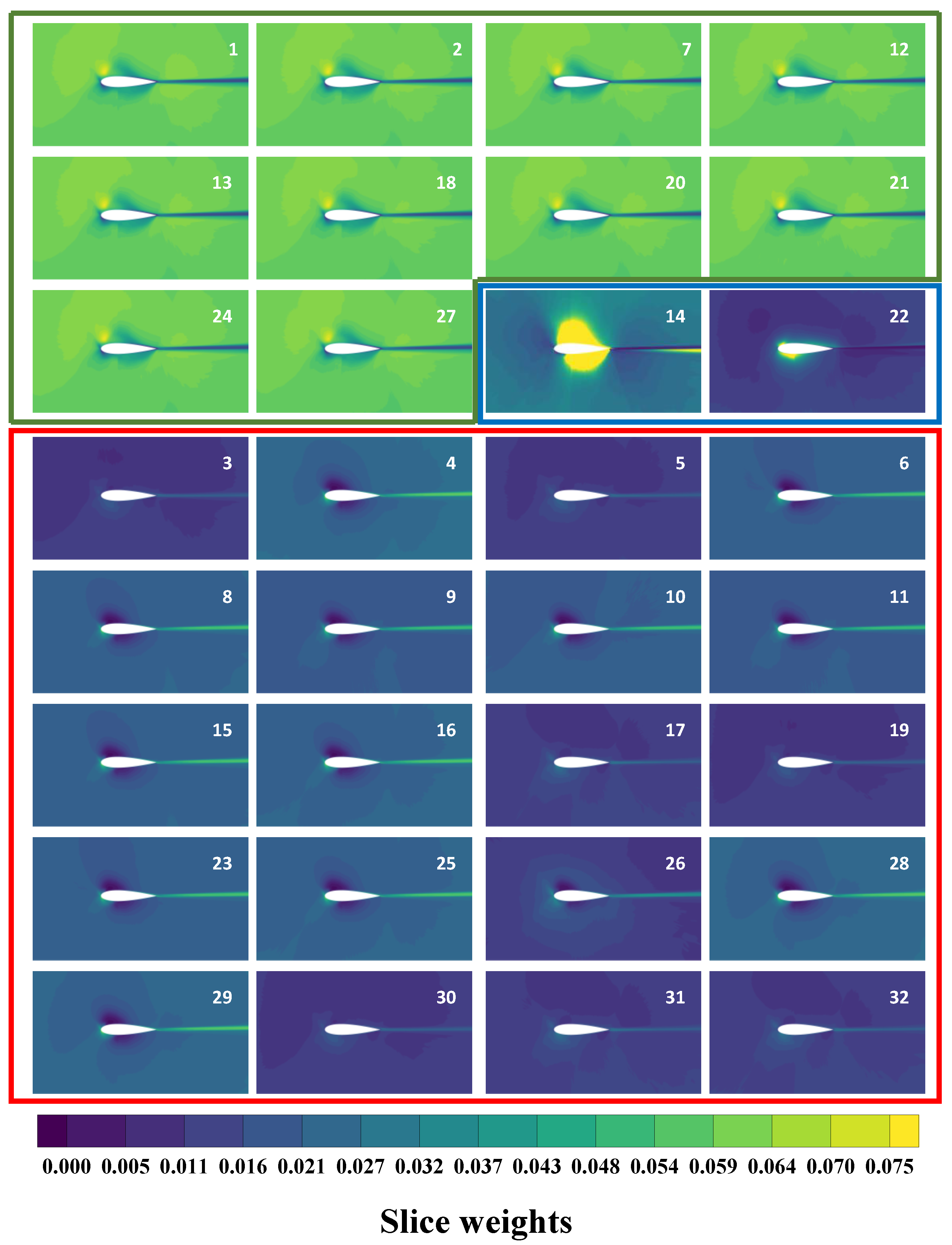
Beyond comparisons with CFD errors, visualizations of the attention distribution in the final Attention layer are used to probe the internal mechanisms of the model. These visualizations assess whether the node attributes produced by the preceding local message-passing layers effectively modulate global feature aggregation in the attention module.

Figure 6 visualizes the slice weights of the final global attention layer. All panels share an identical color scale. The slice number is located in the upper right of each slice. For each slice, the weight map shows where the global module attends. Higher intensities denote nodes that contribute more strongly to the token formed for that slice, as descriped in Equation (13). The resulting patterns closely follow the underlying flow physics, with salient regions aligning with boundary layers, the wake, and far-field zones. Attention distribution can be roughly divided into the following three categories:

• Far-field–oriented slices (green box): These maps allocate low weight to the immediate vicinity of the airfoil and to the wake core, while emphasizing the outer domain. This pattern indicates that the attention layer separates farfield flow from boundary layer and wake dynamics.
• Leading-edge + wake slices (red box): We observe concentrated weight at the leading edge and within the wake, connected by a continuous band from the trailing edge into the wake. This suggests that specific tokens are dedicated to modeling the evolution of shear-layer structures and downstream transport.
• Surface-focused slices (blue box): The weights form narrow rims along the airfoil surface, consistent with a focus on boundary layer processes. The emergence of these near-wall saliency patterns implies that the node embeddings produced by local feature learning effectively condition the global module to attend to the flow areas where the velocity gradients are strongest.

Taken together, these figures demonstrate that the proposed local-first-global-last design produces semantically explicit labeling of the far-field, boundary layer, and wake regions, thus facilitating accurate cross-scale coupling.

3.3. Airfoil Surface and Quantitative Comparison

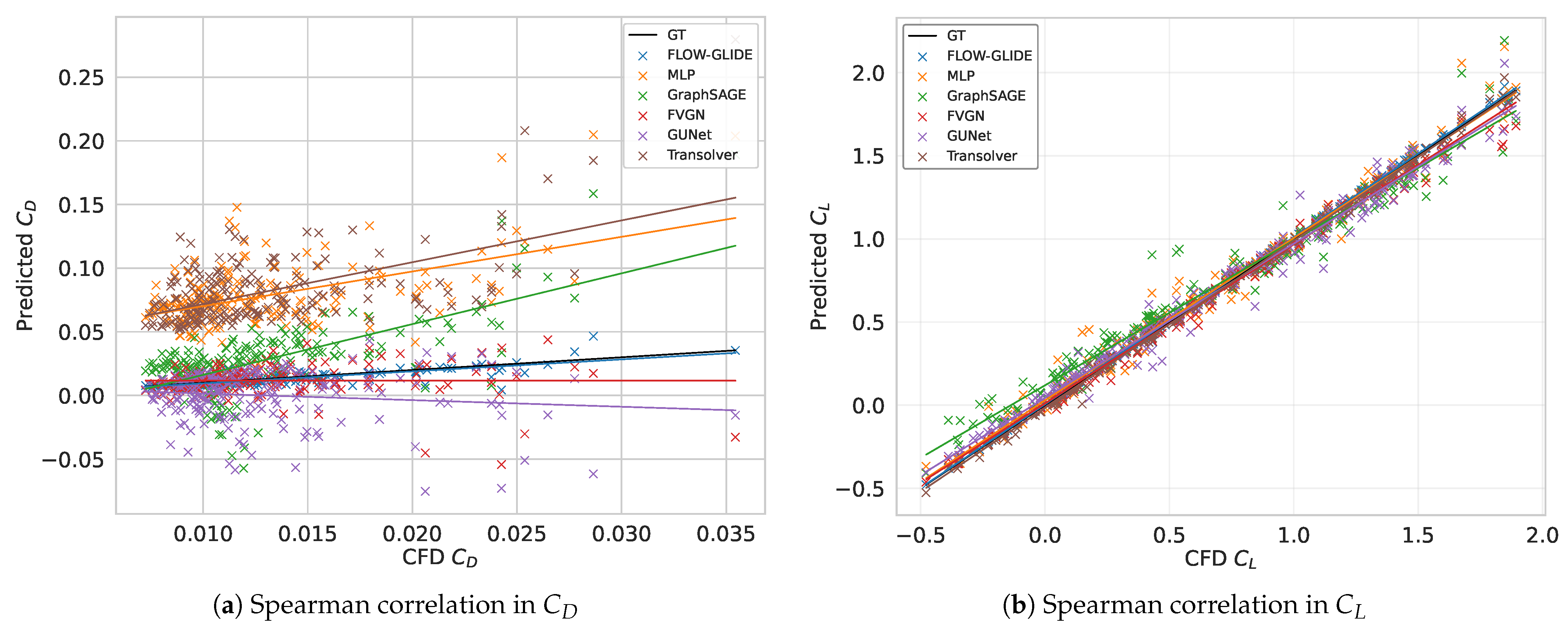
Following the field-level analysis, the evaluation turns to quantitative statistical analysis, encompassing both the airfoil surface and the flow field. Figure 7 shows the correlation between the lift and drag coefficients in each test case, and a linear fit is performed on the results of the entire testset. The black curve is the CFD result, which slope equals one.

Figure 7a presents the spearman correlation of drag coefficient. Among all methods, FLOW-GLIDE exhibits the tightest clustering around the identity with a regression slope closest to one and near-zero intercept, indicating superior calibration and reduced bias across the full drag range. Baselines display either dynamic-range compression, shows a slope less than one, or systematic over-prediction at higher CD. FLOW-GLIDE mitigates both, yielding smaller residuals and higher rank consistency with CFD reference.

For the lift coefficient $C_L$, although all models follow the ground truth closely, FLOW-GLIDE produces a fitted line nearly coincident with the identity and exhibits the smallest scatter across the entire $C_L$ range, including the high-lift regime, indicating excellent monotonic agreement and negligible scale bias.

Figure 8 compares surface pressure distributions predicted by the FLOW-GLIDE and baseline models under two operating conditions: (a) low speed and high angle of attack, (b) high speed and low angle of attack.

At high AoA, FLOW-GLIDE accurately reproduces the magnitude and streamwise location of the leading-edge suction peak and tracks the suction-side pressure-recovery gradient without spurious oscillations. By contrast, several baselines exhibit systematic biases, including under-predicted suction minima, downstream-shifted peaks, and high-frequency ripples over mid-chord, and some additionally show a negative offset on the pressure side.

As shown in Figure 8b, differences are smaller overall in low AoA and high speed condition, yet FLOW-GLIDE remains the closest to CFD across the entire chord on both surfaces. It captures the stagnation jump, the monotonic pressure recovery along the suction side, and trailing-edge closure. Baseline methods reproduce the overall surface-pressure trend but exhibit noticeable offsets relative to CFD, including mild slope and level deviations along portions of the chord.

In addition to visualization, FLOW-GLIDE is quantitatively compared with baseline models across different tasks.

Table 2. Test result on AirfRANS (Full regime, baseline result from AirfRANS, and Transolver).

Model	Volume↓	Surface↓	${\mathit{C}}_{\mathit{L}}$↓	${\mathit{\rho }}_{\mathit{L}}$↑
GraphSAGE	0.0102	0.0660	0.517	0.965
Transolver	0.0037	0.0140	0.103	0.997
PointNet	0.0280	0.0930	0.742	0.938
FVGN	0.0438	0.0230	0.079	0.997
MLP	0.0114	0.1130	0.767	0.913
GNO	0.0269	0.0405	0.201	0.993
GALERKIN	0.0074	0.0159	0.233	0.995
GNOT	0.0049	0.0152	0.199	0.994
GINO	0.0297	0.0482	0.182	0.995
FLOW-GLIDE	0.0014	0.0025	0.036	0.999

summarizes full-regime results on AirfRANS [39]. Downward arrows indicate that smaller is better, and the upward arrow indicates that larger is better. Here, Volume denotes the domain-wise relative-$L_2$ error averaged over the four predicted variables. Surface is the surface relative-$L_2$ error. The volume error was reduced by 62% relative to the strongest baseline, Transolver [30]. The reduction in error for surface metrics was particularly significant, decreasing by nearly an order of magnitude. The lift coefficient also improved by 54% compared to the best performing FVGN [19] and the Spearman rank correlation for $C_L$ is the highest among all methods.

Beyond the full-regime benchmark, out-of-distribution (OOD) generalization is evaluated on two extrapolation tasks: Reynolds number and angle of attack. For Reynolds extrapolation, the training set comprises 500 cases with $\mathrm{Re}\in [3\times {10}^6,5\times {10}^6]$, the test set contains 500 cases drawn from the two held-out outer bands $\mathrm{Re}\in [2\times {10}^6,3\times {10}^6]\cup [5\times {10}^6,6\times {10}^6]$. For AoA extrapolation, the training set includes 800 cases with $\mathrm{AoA}\in [-{2.5}^{\circ },{12.5}^{\circ }]$ and the test set includes 200 cases sampled from the disjoint intervals $\mathrm{AoA}\in [-5^{\circ },-{2.5}^{\circ }]\cup [{12.5}^{\circ },{15}^{\circ }]$. Evaluation uses the same metrics as Section 3.2, and the results are summarized in

Table 3. Performance comparison on Reynolds and AoA task (baseline result from Transolver).

Model	Reynolds		AoA
	${\mathit{C}}_{\mathit{D}}$↓	${\mathit{\rho }}_{\mathit{D}}$↑	${\mathit{C}}_{\mathit{L}}$↓	${\mathit{\rho }}_{\mathit{L}}$↑
MLP	0.6205	0.9578	0.4128	0.9572
GraphSAGE	0.4333	0.9707	0.2538	0.9894
Transolver	0.2996	0.9896	0.1500	0.9950
PointNet	0.3836	0.9806	0.4425	0.9784
GNO	0.4408	0.9878	0.3038	0.9884
CALERKIN	0.4615	0.9826	0.3814	0.9821
GNOT	0.3268	0.9865	0.3497	0.9868
GINO	0.4180	0.9645	0.2583	0.9923
FLOW-GLIDE	0.3344	0.9985	0.1987	0.9958

.

Table 3 reports OOD results. For the Reynolds-number extrapolation task, FLOW-GLIDE attains the highest rank consistency with ${\rho }_D=0.9985$, surpassing the best baseline. In terms of absolute drag error, FLOW-GLIDE is competitive, ranking behind Transolver [30] and GNOT [43] but outperforming the remaining baselines. For the AoA extrapolation task, FLOW-GLIDE also achieves the best Spearman correlation with ${\rho }_D=0.9958$. For absolute lift error, it is second best, close to Transolver [30] and lower than all other baselines. Overall, FLOW-GLIDE exhibits the strongest rank consistency and competitive absolute accuracy across both extrapolation tasks.

3.4. Ablation

Two ablation studies are conducted to evaluate the benefits of the interleaved Local–Global design and to determine the local depth required to avoid over-smoothing while preserving discriminative locality. The first ablation removes interleaving: message-passing and attention layers are stacked in contiguous blocks, varying only their order to form GN-Attention and Attention-GN. Consistent with Section 3.2, the reference FLOW-GLIDE stacks four MAG-BLOCKs, each comprising three Message Passing layers followed by one attention layer. To match the total depth and parameter count, GN→Attention uses twelve Message Passing layers followed by four attention layers, whereas Attention→GN applies the reverse ordering. All other hyperparameters are kept fixed to enable a fair comparison.

Table 4. Comparison of model performance in different order (full regime).

Model	Volume↓	Surface↓	${\mathit{\rho }}_{\mathit{D}}\uparrow$	${\mathit{\rho }}_{\mathit{L}}\uparrow$	${\mathit{C}}_{\mathit{D}}\downarrow$	${\mathit{C}}_{\mathit{L}}\downarrow$
GN-Attention	0.0015	0.0028	0.5294	0.9994	0.1977	0.0288
Attention-GN	0.0214	0.0784	0.5040	0.9957	0.7783	0.1211
FLOW-GLIDE	0.0014	0.0025	0.7921	0.9996	0.1368	0.0368

compares FLOW-GLIDE with non-interleaved architectures. With total depth and training setup held fixed, FLOW-GLIDE delivers the best overall performance. Compared to GN-Attention, FLOW-GLIDE reduces $C_d$ by 31%, increases ${\rho }_d$ by 50% and further decreases Volume/Surface by 6.7%/10.7%, respectively. Attention-GN underperforms across all metrics, indicating that global-first ordering washes out near-wall gradients early. The subsequent GN layer cannot recover the lost high-frequency information. In terms of volume and surface metrics, Attention-GN is one order of magnitude lower than FLOW-GLIDE. Compared to FLOW-GLIDE, ${\rho }_D$ and $C_D$ in Attention-GN decreased by 57% and 82%, respectively. A caveat is that GN→Attention achieves a slightly lower $C_L$ error than FLOW-GLIDE. In the Volume and Surface metrics, the GN→Attention configuration performs comparably to FLOW-GLIDE, demonstrating the importance of prioritizing local feature learning over global feature learning. Furthermore, with the exception of $C_L$, GN-Attention performs worse than FLOW-GLIDE in all other metrics, further demonstrating that overly deep graph networks can lead to oversmoothing. The appropriate number of GN layers was further investigated in a second ablation experiment. Overall, the ablation supports interleaving local message passing with global attention, which better balances near-wall fidelity and long-range coupling.

The second ablation focused on determining how many Message Passing layers are needed in a MAG-BLOCK to capture local features as closely as possible without causing oversmoothing. The number of Message Passing layers per block is varied, with $k\in 1,2,3,4,5$, while all other factors are kept fixed. Models are then evaluated on the full-regime task using the same metrics as Section 3.2, enabling an isolated assessment of how local depth within a block affects performance.

Table 5. Comparison of GN layer in one MAG-BLOCK (full regime).

Number of GN	Volume↓	Surface↓	CL↓	CD↓	${\mathit{\rho }}_{\mathit{L}}\uparrow$	${\mathit{\rho }}_{\mathit{D}}\uparrow$
1	0.0015	0.0032	0.0406	0.2186	0.9995	0.3821
2	0.0021	0.0045	0.0544	0.2884	0.9991	0.2992
3	0.0014	0.0025	0.0366	0.1368	0.9996	0.7921
4	0.0023	0.0028	0.0477	0.1597	0.9993	0.6871
5	0.0019	0.0047	0.0288	0.1657	0.9995	0.5972

summarizes the ablation on the number of Message Passing layers per MAG-BLOCK, with all other settings held fixed. The configuration with $k=3$ delivers the best overall performance. Increasing Message Passing layer from $k=1$ to $k=3$ markedly improves the representation of flow field. However, pushing the layer depth to $k=4$ and $k=5$ introduces oversmoothing, which degrades Volume, Surface, and $C_D$ and substantially lowers ${\rho }_D$. Although $k=5$ yields the lowest lift error $C_L=0.0288$, this comes at the expense of higher field errors and weaker drag rank consistency, and is therefore not preferable overall. In summary, three Message Passing layers strike the most effective trade-off between capturing local structure and avoiding oversmoothing.

4. Conclusions

To address the challenge of balancing strong near-wall gradients and global long-distance coupling in high-Reynolds number flows, this paper proposes MAG-BLOCK, which couples low-level message passing with physical perception attention through residual mapping, further stacking results in the alternating Local–Global architecture FLOW-GLIDE. This design balances discriminative local features with global dependencies in the latent space. Visualization of the final attention layer reveals that tokens form a semantic division of labor across the boundary layer, wake, and far field, providing a mechanistic explanation for the performance improvement.

Comprehensive experiments on AirfRANS validate the approach. In the full-regime track, FLOW-GLIDE reduces the volume relative-$L_2$ error by 62% over the strongest baseline and lowers surface-pressure error by nearly an order of magnitude. It also achieves the lowest lift-coefficient error and the highest Spearman rank correlation among all competitors. Qualitatively, the model reproduces the leading-edge stagnation pattern, suction-side acceleration, and the trailing-edge recirculation bubble with correct curvature and re-attachment location. In out-of-distribution evaluations, FLOW-GLIDE attains the highest rank consistency for both Reynolds-number and AoA extrapolations while maintaining competitive absolute errors, demonstrating robustness when operating outside the training ranges.

Ablation studies clarify architectural choices. Removing interleaving degrades performance, indicating that alternating local message passing with global attention is crucial for suppressing wake-core and near-edge errors without inflating farfield artifacts. Varying the number of message-passing layers per block shows that three layers strike the best balance. Deeper stacks begin to over-smooth and harm drag ranking, whereas shallower stacks underfit local structure.

These results suggest that FLOW-GLIDE is a practical surrogate for rapid design space exploration, inverse design, and control where both accurate ranking and low field-level error matter. The method integrates naturally with mesh-based pipelines and preserves original connectivity, enabling deployment alongside existing CFD workflows as a fast pre-screening or co-simulation module.

Future work will target the attention mechanism by explicitly decomposing global attention into tangential and normal direction. This design aims to learn direction-dependent transport and diffusion. Moreover, physical constraints can be applied to loss functions to enhance physical consistency and interpretability. We also plan to evaluate scalability and generalization capabilities with respect to mesh resolution and problem classes, extending the framework from two-dimensional, stable, incompressible cases to three-dimensional, unsteady, and compressible flows. Together, these directions aim to enhance the inductive bias of FLOW-GLIDE, improve its robustness across domains, and broaden its applicability to practical aerodynamic design and control.