Abstract
This paper introduces a novel scheduling model that integrates weather-based productivity coefficients into multi-unit construction projects, aiming to enhance profit and reduce delays. The method is suitable especially for renewable energy, open-area projects. The authors propose a flow-shop optimization framework that considers key aspects of construction contracts, e.g., contractual penalties, downtime losses, and cash flow constraints. A proprietary Tabu Search (TS) metaheuristic algorithm variant is used to solve the resulting NP-hard problem. Numerical experiments on multiple test sets indicate that the TS algorithm consistently outperforms other methods in finding higher-profit schedules. A real-world wind farm case study further demonstrates substantial improvements, transforming an initially loss-making operation into a profitable venture. By explicitly accounting for weather disruptions within a formalized scheduling model, this work advances the understanding of reliable project planning under uncertain environmental conditions. The solution framework offers contractors an effective tool for mitigating scheduling risks and optimizing resource usage. The integration of weather data and cash flow management increases the likelihood of on-time and on-budget project delivery.
1. Introduction
Efficient scheduling of construction projects is a key challenge for both practitioners and researchers. Significant delays and cost overruns often stem from uncertainties in the external environment, such as unfavorable weather conditions or fluctuating resource availability. The scale of these issues become more significant and complex when dealing with multi-unit construction projects, where each unit (e.g., building, turbine, or road segment) requires an identical or similar set of tasks [1,2,3,4,5]. Scheduling theory, particularly flow-shop problem modeling, offers valuable insights into these challenges [1,4,5,6]. However, further improvements are necessary to capture important factors such as the impact of weather phenomena on work efficiency.
Prior studies highlight the substantial influence of weather on construction schedules. Researchers have examined how temperature, rainfall, wind speeds, and snowfall can reduce the productivity of work crews, especially in the construction sector where most of the works are performed without any shelter [7,8,9,10]. These analyses confirm that weather-related disruptions can significantly extend project duration and increase costs.
Onshore wind farm construction projects are especially vulnerable to weather conditions due to their localization in windy and open areas. Built as a cluster of turbines they are a model example of multi-unit construction projects. Currently, the most commonly recommended approach to the issue of scheduling the implementation of wind farms is the use of the CPM critical path method with visualization of the schedule in the form of Gantt charts. It is recommended for the creation of schedules for such projects by, for example, AACE International (Association for the Advancement of Cost Engineering), an organization dealing with the establishment of recommended practices regarding project management, e.g., practices in the construction industry related to the implementation of wind farms [11]. However, CPM and Gantt charts are not designed to account for weather uncertainty during construction work and to model weather factors that affect work performance. In construction practice, the problem of weather influences is estimated on the basis of the previous experience of contractors by establishing a set of rules that are designed to properly take into account these impacts on the performance of works [12]. However, such a subjective approach to this problem may cause significant deviations in the actual deadlines for the completion of works in relation to the deadlines planned in the schedule [12]. Current scientific research on the issue of the impact of weather on the construction schedule of onshore wind farms is not extensive compared to research on offshore wind farms. In the paper [12], the authors proposed fuzzy modeling to account for the uncertainty of wind speed only during the construction of a wind farm. In the paper [13], a simulation approach of weather events during the installation of a wind turbine using a weather generator is presented. The article [14] proposes mathematical optimization of the wind farm construction schedule with resource constraints, taking into account wind speed and precipitation. The few studies described above concern the creation of schedules for the construction of onshore wind farms in the early planning phase of their implementation. They do not apply to advance short-term planning with regard to weather influences, which covers the next few days to about 2 weeks. The problem of developing such schedules during the implementation of onshore wind farms is addressed in only one article [15]. It presents a hybrid simulation model of the duration of works using weather forecasts for the coming days (wind, precipitation, temperature). According to the authors, this makes it possible to create short-term advance schedules that will improve the process of planning and controlling the entire course of the implementation of such farms.
This paper addresses the scheduling problem of multi-unit onshore wind farm construction projects under varying weather conditions. The intention of the authors of the article is to create a tool for early, deterministic planning of the implementation of such farms using flow-shop modeling known from scheduling theory. The existing and described models for creating early schedules [11,12,13,14] do not take into account the impact of changes in the order of execution of individual wind farms in a given farm on the scheduling result. Taking into account the possibility of changing the order of execution of facilities in a multi-facility project such as an onshore wind farm has a fundamental impact on the value of the adopted criterion in the schedule, which is presented in the articles [1,4,5]. Such an opportunity is provided by modeling the process of implementation of the onshore wind farm that is the subject of this article as a variation in the flow-shop problem and searching for optimal schedules among the set of possible permissible schedules. Another issue raised in the article is the need to take into account all possible weather influences on the schedule of the implementation of such farms. In the few studies on this problem and presented in articles [12,13,14], only selected weather phenomena such as wind speed and rainfall have been used as influencing the efficiency of works. This may be insufficient to properly assess the impact of weather on the performance of works. For this reason, in this article, in order to comprehensively take into account all possible weather influences that may occur during the construction process of onshore wind farms (the appearance of wind at a speed that makes it impossible to carry out assembly works, rainfall of varying intensity, snowfall, the occurrence of thunderstorms with lightning), the model presented in the article [8] has been chosen. According to the authors, it is the most suitable method (among those presented in Section 2.1) for scheduling the implementation of onshore farms located in the northern part of Polish (due to the possibility of occurrence of all the above-mentioned weather phenomena in this area).
The goal of the proposed model of scheduling is to maximize the contractor’s profit, modeled as the total cash flow at the project’s final billing cycle. The scheduling model integrates weather-related reduction coefficients based on historical data. This allows for capturing problematic productivity fluctuations more accurately.
Due to the NP-hard nature of the problem, a metaheuristic Tabu Search (TS) algorithm was deployed to find feasible, high-quality solutions [16,17].
The paper is structured as follows: Section 2 presents a comprehensive literature review of the impact of weather on construction and the methodologies used for scheduling multi-unit projects. Section 3 introduces the optimization model, including the key parameters and constraints that define the multi-unit scheduling task. Section 4 outlines the proposed Tabu Search approach, while Section 5 details the testing of its accuracy and compares results with those from alternative algorithms. A real-world case study involving wind farm construction is provided in Section 6 to validate the effectiveness of the proposed solution.
2. Literature Review
The literature review on the issues in this article has been divided into two subsections. The first concerns the impact of weather on the efficiency of construction works. The second one presents a review of the current literature on the issue of scheduling multi-unit projects.
2.1. Impact of Weather Phenomena on the Efficiency of Construction Works
The issue of the impact of weather phenomena on the efficiency of construction works and thus the duration of works has been described by researchers in many articles. Ref. [9] presented the issue of the influence of weather conditions on the length of the working day in a construction project. The authors’ model operated on hourly weather data that had been collected over the past 10 years. The following factors were taken into account: the possible impact of too low and too high temperatures in combination with strong wind and humidity, the impact of precipitation and snow. The use of the weather model is limited to masonry, electrical and outdoor works (e.g., finishing).
A model to calculate the influence of weather on the duration of works and construction projects was also proposed by AbouRizk & Wales [18]. The method given by the authors is based on simulating the course of the project day by day. On a given day of the project, coefficients are generated to correct the current performance of works based on the current weather (rainfall, temperature). On this basis, the duration of the activity is calculated, and then the total time of the project.
In their article, El-Rayes & Moselhi [19] presented the consideration of the impact of the amount of rain falling during the working day on the efficiency and duration of roadworks in the construction of motorways. The results obtained were positively verified with the results obtained by two other models used for this type of work.
The impact of weather (among other factors) on the risk of a construction project is presented in another article [20]. In this work, fuzzy sets were used to estimate the impact of individual factors. The main risk factor was ambient temperature.
Marzouk & Hamdy [21] presented an application for forecasting performance losses caused by weather influences (rain, temperature) during the assembly and disassembly of reinforced concrete formwork of monolithic structures. It uses historical weather data, fuzzy modeling, and dynamic systems. The authors tested the effectiveness of their model on weather data from Egypt (Cairo and Alexandria).
The impact of extremely cold weather on the duration of tunnel construction is presented in the article [10]. The problem model uses stochastic processes to generate new weather factors such as minimum and maximum temperature, precipitation, and wind speed to forecast the duration of activities based on the location and date of the work.
The impact of many factors, including precipitation, temperature and humidity, on the duration of works for concrete frame structures is presented in the article [22]. The authors have developed a tool based on artificial neural networks, which is used to determine the duration of activities for the implementation of this type of building structures.
Senouci & Mubarak [23,24] also studied the issues of optimal scheduling of construction projects, taking into account the impact of extreme weather. In their works, the CPM critical path method was used for scheduling, and a genetic algorithm was used to optimize schedules. The influence of weather was taken into account in the calculation of the duration of the activity and its cost by applying arbitrary correction coefficients adopted for the weather conditions of the Middle Eastern countries. The article [25] develops these ideas further by modeling the impact of extreme weather in Qatar on the efficiency of formwork, masonry, plastering and cladding works. The analyzed factors included: temperature, humidity and wind. Linear regression models have been developed based on historical data to predict job performance on a given day of the year. A summary of the literature review on the study of the relationship between weather and labor productivity in construction was developed by Al Refaie et al. [7].
A stochastic model for determining the duration of a construction project taking into account the impact of weather conditions was presented in Ref. [8]. Modeling of the duration of the project was based on historical weather data and included its different aspects (temperature, rainfall intensity, wind, storm). This data was used to determine the coefficients reducing the efficiency of works (on a monthly basis). Productivity for specific works was reduced by assuming the number of days in a given month during which these works were impossible to carry out (due to the weather conditions).
Unfortunately, the models for determining the impact of weather on productivity and thus the duration of construction works proposed in Refs. [9,10,18,19,20,21,22,23,24,25] take into account only selected weather factors: articles [9,18,21,22]—precipitation, temperature; articles [10,19]—precipitation; article [20]—temperature; articles [23,24,25]—extreme conditions (high temperature, precipitation, storms). In each of these articles, the authors stipulate that the models provided by them may be used only for strictly defined types of construction works: masonry, electrical installation, finishing [9], road works [19], concrete works [20,21,22], tunneling [10]. In addition, the models presented in articles [23,24,25] can only be used in weather conditions characteristic of the countries of the Middle East. In connection with the above limitations of these studies, the authors of this article paid special attention to the article [8]. It presents a model for describing the influence of weather for climatic conditions that are characteristic of European countries, including Poland. This article proposes a way to determine the impact of all possible weather factors that can be observed in the northern part of Poland. The onshore wind farm that is the subject of the case presented in Section 6, is located in this region. In addition, the method presented in Ref. [8] is suitable for all types of works that occur during the implementation of onshore wind farms (earth, road, concrete, assembly, electrical, masonry, finishing). The details on required calculations are provided in Section 3.
2.2. Multi-Unit Construction Project Scheduling Problem
The construction project scheduling problem continues to occupy the attention of researchers from all over the world. Due to the way the works are performed, we can divide these projects into “non-repetitive” and “repetitive”. For the non-repetitive projects CPM/PERT network planning is most often used to create a schedule [26].
Non-repetitive projects most often concern cubature construction related to residential, service or industrial buildings. Repetitive projects are characterized by the possibility of dividing them into parts (units), for example, work zones, sections of a specific size (e.g., length), individual floors of buildings, or entire buildings (in case of multi-object projects). Each part of a given project requires the performance of the same or a similar set of activities using the available resources, for example, work crews. Examples of repetitive projects may be single-family housing estates, high-rise multi-story buildings, pipeline networks, roads, highways.
In order to create a schedule of repetitive projects, many methods are used, e.g., LOB (Line of Balance) [27], the LSM (Linear Scheduling Model), the RSM (Repetitive Scheduling Method) [28] based on the LOB technique, and TCM methods [29].
A comprehensive literature review of current research on the scheduling of repetitive projects was presented by Tomczak & Jaśkowski [30]. Among the repetitive projects, the so-called multi-unit projects stand out, which involve the implementation of many construction objects such as buildings or engineering structures, e.g., road sections.
To create scheduling models for multi-unit projects, the scheduling theory is often used, especially the flow problem [6], which is a case of discrete optimization. The aim of the current research on this type of projects is to improve optimization models describing multi-unit projects by taking into account new factors influencing the shape of the schedule and better reflecting the situation of a given multi-unit project. Bożejko et al. [31] presented the problem of optimal scheduling of a multi-unit project consisting in the construction of many production halls. The task of discrete optimization in this model was to find the optimal sequence of hall construction, taking into account the criterion of the total cost of their implementation. The value of this criterion consisted of the determined costs of works and possible penalties for exceeding the directive deadlines for the completion of works. To solve the discrete optimization problem, the scatter search algorithm was used.
The fuzzy approach in scheduling a multi-unit project was used by Bożejko et al. [32]. It considered the NP-difficult problem of scheduling a construction project with the cost criterion of the sum of penalties for exceeding the directive deadlines. The parameters in the project were fuzzy or constituted random variables with different distributions.
The possibility of performing works by more than one working group was analyzed in Ref. [16]. The author additionally proposed the directed graph expression of the sequential relations between the activities in the undertaking. The tabu search algorithm was used to solve the optimization task.
Podolski & Sroka [1] presented the issue of minimizing the total cost of a multi-unit project with the assumption that the relationship between the duration of the activity and its cost is linear. The adopted optimization criterion was determined on the basis of a mathematical programming model and took into account direct and indirect costs, the costs of failure to meet directive deadlines and the costs of discontinuity of work groups of work. A modified simulated annealing algorithm was used to find the optimal solution in this scheduling model.
Optimal scheduling of multi-unit projects was also the subject of papers written by Tomczak & Jaśkowski [2,3]. In the first one, the purpose of scheduling was to minimize the overall project duration, the duration of buildings, and the idle time of resources. A particle swarm algorithm was used for optimization. In the second, the authors use a two-criteria scheduling model using the possibility of changing the order of execution of objects. Similarly, a particle swarm algorithm was used for optimization.
The total profit of the investor is a criterion of the multi-unit project model by Sroka et al. [4]. The authors calculated this profit as a result of the total cumulative cash flows from the entire project. Their model takes into account monthly cash flows including direct and indirect costs, penalties for missed deadlines, costs of workgroup interruptions and losses on loans. Proprietary forms of metaheuristic algorithms (simulated annealing and genetic search) were used in this article to search for the optimal solutions.
Another factor that has a significant impact on the shape of the schedule of a multi-unit project is the learning and forgetting effect [5]. The criterion examined by the authors was the cost criterion of the entire project, and the optimization task was solved using the proprietary form of the simulated annealing algorithm
3. Materials and Methods: New Optimization Model for Scheduling the Onshore Wind Farm Construction Project
The article discusses the problem of scheduling a multi-unit project, which consists of the implementation of a wind farm (power plant) located on land. This issue can be described as follows. A set of n construction objects (wind turbines) is given, which are to be made with m different working groups. Each of the n wind turbines requires m different activities. Each of the m working groups can perform only one type of activity, e.g., earthworks, concrete or assembly works. It is assumed that the order of transition of working groups during the construction of subsequent turbines is the same for each working group and this order can be arbitrary, i.e., in the sense of the theory of scheduling tasks, it is a permutation problem that belongs to discrete optimization problems. In addition, the sequence of activities during the construction of subsequent turbines is also the same and results from the technology of construction works.
In the analyzed type of a multi-unit project, the duration of activities performed by m different working groups in n wind farms is determined on the basis of the labor intensity of a given activity and the efficiency of a given work group. The article assumes that the efficiency of working groups depends on the weather conditions that prevail at a given time of carrying out works. It is assumed that the following weather conditions may occur, which, if they occur, significantly reduce the efficiency of works in a given calendar month. The weather conditions considered are: negative temperature, rainfall, strong wind, snowfall, storm. Each of these conditions is taken into account for a given type of work by calculating (on the basis of historical data) an appropriate efficiency factor reducing the assumed maximum efficiency of the work. This effect will extend the duration of activities in the project. Hence, taking into account the start date of the project (the selected month of its commencement) have a significant impact on the date of its completion. This is especially important for very long construction projects which may take years to complete. Such projects may have a significant impact on construction companies in terms of potential contractual penalties and court disputes fees [33,34].
The considered function of the optimization goal is to maximize the total profit achieved in the project, and more specifically the accumulated cash flow on the last day of the project. It takes into account the costs incurred during the implementation of the project: direct costs of working groups, indirect costs, contractual penalties for exceeding the deadline for completion of construction, penalties related to interruptions in the work of working groups, costs of loans. The presented discrete optimization problem is a generalization of the classic permutation flow shop problem, the model of which is presented schematically in Figure 1. In the terminology of scheduling theory, it is denoted as an FǀǀCmax problem, according to notation proposed by Graham et al. [35]. The cardinality of the set of possible solutions to the permutation flow shop problem is n! and this is an NP-difficult problem.
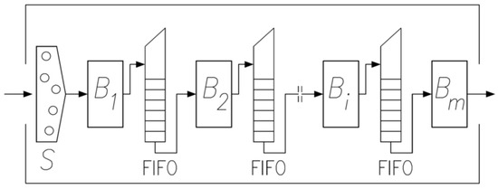
Figure 1.
Permutation flow-shop system; S—input sequence (permutation) of n tasks (construction object) to the system of working groups B1, …, Bm. The cardinality of the set of possible solutions is n! (n—number of construction objects).
The proposed optimization model of the multi-unit project which can be used for the construction of a wind farm is as follows.
Parameters:
- The project creates a set of wind turbines Z = {Z1, Z2, Z3, …, Zi, …, Zn}.
- There are work groups to perform all the work in the project, each of which performs one type of work. They form the set B = {B1, B2, B3, …, Bj, …, Bm}.
- Each object Zi ∈ Z requires the implementation of m activities (each representing a given type of work) that form the set Oi = {Oi,1, Oi,2, Oi,3, …, Oi,j, …, Oi,m}.
- It is assumed that the activity Oi,j ∈ Oi can be carried out by the working group Bj. The duration of the activity Oi, is pi,j > 0. The set of durations pi of the action from the set Oi is given by the vector ti = [ti,1, ti,2, ti,3, …, ti,j, …, ti,m]. The duration of activities ti,j are determined on the basis of the workload (expressed in man-hours or machine hours) determined on the basis of the normative base (historical data) and the size of the working group (number of employees and machines). During the implementation of the project schedule, the duration of the ti,j activity is modified by the weather performance coefficient depending on the weather conditions.
- The direct cost of materials and equipment used for the implementation of activities Oi,j by the Bj working group is determined by the variable ci,j ≥ 0. The set of possible costs of works ci from the set Oi are defined by the vector ci = [ci,1, ci,2, ci,3, …, ci,j, …, cj,m]. The cost of the activity ci,j is determined by calculating the costs of performing the work Oi,j by the Bj working group belonging to the contractor’s resources.
- The cost of labor for the performance of activities by the Bj work group is determined by the variable ≥ 0.
- The indirect cost of performing works is determined by the variable ≥ 0.
Constraints:
- The sequence of performing activities results from the chosen technology of construction works:
- It is assumed that each workgroup in the Bj team can perform only one activity in a given facility at any given time.
- It is assumed that the activity Oi,j ∈ Oi is carried out continuously by one working group Bj for the duration of ti,j > 0.
The decision variable is the order π of execution of objects, which is the same for each of the working groups (permutation of execution of objects π = (π(1), π(2), …, π(j), …, π(n))) and the selection of the month k of the start of works (k = (1, 2, …, 11, 12)). The number of the set of possible solutions in the model is equal to 12n!.
The deadlines for the completion of individual activities can be determined according to the following formula:
where i = 1, 2, …, n, j = 1, 2, …, m, π(0) = 0, F0,j = 0, Fi,0 = 0.
Fj,π(i) = max{Fπ(i − 1),j, Fπ(i),j − 1} + tπ(i),j,
The duration of the entire project Fn,m (the time of execution of all works in all power plants) is Fn,m = Fπ(n),m.
The weather productivity coefficient is calculated on the basis of Ref. [8]. At the beginning, Raw Climatic Coefficients (RCCs) are calculated based on historical data. They show the number of days without a given weather phenomena which is unfavorable for the conduct of works. RCCs for different weather factors Ck are calculated as follows:
The effect of temperature below 0 degrees Celsius:
Impact of rainfall above 10 mm per day:
Impact of rainfall above 30 mm per day:
Impact of wind speed above 33 km/h (10 m/s):
Impact of snowfall:
Impact of thunderstorms:
Then, for different types of work, Climatic Reduction Coefficients (CRC) are calculated, which are later used as for corresponding types of works. CRCs are coefficients that range from 0 to 1 and show how much the performance of a given type of robot decreases. For example, CRCs for four types of works: earthworks, concrete (formworks and concreting), and assembly can be calculated as follows [8]:
For earthworks:
For concrete works—formwork:
For concrete works—concreting:
For assembly works of the steel structure of a wind power plant:
The objective function in this model aims to maximize the cumulative cash flow at the end of the project’s final billing period [5]. This value reflects the contractor’s overall profit. The function will be optimized to achieve the highest possible cash flow (maximization). The objective function includes the following variables:
- —completion time of tasks carried out by a work group j on unit i,
- —final completion time of all construction activities,
- h—billing cycle index, where , and H denotes the final billing cycle (period),
- k—the number of the calendar month in the project,
- TI—timespan (in days) representing the duration of a single billing period,
- —the initial (minimum) duration of the activity Oi,j without taking into account the influence of the weather,
- —total time required by work group j to complete all tasks on a unit i, dependent on the weather performance coefficient
- —time spent by work group j on a unit i during billing period h,
- —idle time or work interruption for crew j within billing cycle h,
- —deadline for finishing tasks on unit i,
- —delay associated with completing tasks on unit i in billing period h,
- —direct cost of works carried out by crew j to complete unit i,
- —daily indirect cost per unit,
- α—discount rate applied per billing interval,
- Pro—profit margin, expressed as a percentage,
- —penalty cost per unit for delays in completing work on a unit i,
- —penalty cost per unit for idle time (discontinuities) experienced by crew j,
- —penalty applied as a percentage for periods with negative cash flow,
- —binary variable indicating whether a penalty for negative cash flow is applied in billing period h,
- —lag (in billing cycles) before income is recorded,
- —lag (in billing cycles) before penalties are recorded,
- —cumulated cash flow for billing period h,
- —indirect costs incurred during billing period h,
- —direct costs incurred during billing period h,
- —production cost during billing period h,
- —value of production achieved during billing period h,
- —total penalty for a delay of works in billing period h,
- —total penalty for a downtime (discontinuities/work interruptions) of work groups during billing period h.
Based on the defined parameters, constraints, and variables, a mathematical programming model was developed by the authors and expressed as follows:
s.t.:
The objective function (13) was designed to maximize the total cumulative cash flow at the project’s final billing cycle, representing the contractor’s total profit (TP). The number of billing cycles (14) is determined based on the duration of the time intervals and the completion time of the construction activities. Formula (15) outlines a recursive approach for computing cumulative cash flows across subsequent billing periods.
When cash flow becomes negative, it creates a need for external financing to continue project operations. This typically involves the contractor securing interest-bearing loans or foregoing potential investment returns on their own capital. A binary variable (16) represents this scenario by applying penalties in periods where negative cash flow occurs.
The production cost (17) in each billing cycle is calculated as the present value of both indirect (18) and direct (19) costs. The production value is invoiced at the close of each billing period and, after a predefined delay () disclosed in the contractual documents. It becomes the contractor’s income from the client. This value is also discounted. Penalties for work delays (20) and crew downtime (21) are likewise applied with a delay. Delay penalties are usually defined in the contract between the client and the main contractor and often range from 0.05% to 0.2% of the gross contract amount for each day overdue. Downtime-related penalties stem from the contractor’s obligation to keep work groups (crews) on standby, ready to resume work at any time [5]. Equation (22) models weather impact on the duration of construction works.
The presented model is visualized as a disjunctive graph G(π). An example, including critical path, is illustrated in Figure 2. The structure of such graph depends on the selected decision variable π: G(π) = (N, E(π)), where N denotes the set of nodes and E(π) represents the set of arcs (edges). The set of nodes N = {1, …, i, …,n} × {1, …, j, …, m} correspond to tasks performed across different project units. Each node has a set weight (i, j) representing the duration of the task tπ(i),j. The E(π) = EF ∩ ES(π) set is dependent on the chosen decision variable π. Horizontal arcs from the set ES(π), reflecting the sequence of task execution across units, link nodes π(i − 1) and π(i) for i = 1, …, n. Vertical edges from the set EF, representing technological dependencies, connect task j with its predecessor j − 1.
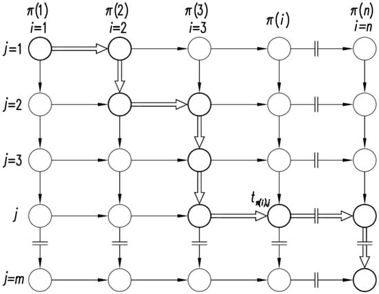
Figure 2.
The graph for the described model of the project with the marked critical path.
The model of a multi-unit project presented above represents a NP–hard discrete optimization problem. This is due to the assumption of a permutational flow problem (the FǀǀCmax problem), which is NP–hard. To solve optimization tasks in the presented model, authors proposed a proprietary metaheuristic algorithm using the tabu-search algorithm (TS).
4. Optimization Method for the Presented Multi-Unit Model
The Tabu Search method (TS) was proposed by Glover [36,37]. It replicates the natural process of searching for a solution to a problem carried out by humans. The basic version of the TS algorithm starts with a specific starting solution. Then, for this solution, the local neighborhood is found. The neighborhood is defined as a set of solutions that can be achieved after making moves in a given solution space, i.e., transformations transforming a given solution into another according to established rules. The neighborhood is searched for a solution with the lowest value of the objective function. This solution becomes the baseline solution for the next iteration. The result of the algorithm’s operation is the best solution from the search trajectory.
The essence of the TS method lies in the use of search history, which prevents the trajectory from stopping at the local optimum and allows it to venture into more promising search areas. Most often, short-term memory called a tabu list is used for this purpose. This list stores for a limited time the most recent attributes of solutions, the movements leading to these solutions, or the attributes of the movements of the most recently considered solutions. This is usually performed by entering a fixed list length, which removes the oldest element when a new item is added. The attributes of the elements in this list indicate that some future moves may not bode well and will therefore be considered prohibited. This prohibition can be revoked if the so-called aspiration function deems the move beneficial. This is an additional function whose value for a given solution can cause the moves leading to the solution or its attributes not to be on the tabu list. The conditions for the termination of the algorithm’s work can be: time limit, maximum number of iterations, reaching a satisfactory value of the goal function or optimal value. Despite the fact that its invention took place over 30 years ago, TS algorithm and its variations are still often used in various modern optimization problems [16,38,39,40].
Below, a general algorithm of TS method used to solve flow shop problems in scheduling theory is presented in the form of a flowchart (Figure 3).
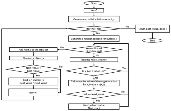
Figure 3.
TS algorithm flowchart.
In the algorithm used, the neighborhood was generated in two different variants. Variant 1 was a solution that differed in the month of commencement of the works by +/−1 from the current solution (with the same order of construction of the objects). Variant 2 changed the order in which the objects were to be constructed randomly swapping two objects in a permutation (also with the same month of starting the works). There were 5 such 2 variants. The neighborhood consisted of 7 cases differing in the order of construction of the facilities or the month of commencement of works. The stop condition was to achieve the assumed number of iterations of the algorithm (m = 6: 90 iterations, m = 10: 130 iterations, m = 15: 250 iterations, m = 20: 650 iterations, Case study: 500 iterations). The size of the tabu list was 10 in each case.
5. Testing the Accuracy of the Results Obtained Using the TS Algorithm
The article uses the metaheuristic Tabu Search algorithm to solve discrete optimization tasks. An important element of the research is to check the accuracy of the results obtained with this algorithm by comparing the results obtained with other algorithms. The experimental analysis method was adopted to verify the tabu search algorithm due to the popularity of this method and ease of application [17,41]. This method consists of a posterior assessment of the behavior of the studied algorithm (or more precisely, the approximation error) on a limited, representative sample of specific examples. This sample is usually created by randomly generating examples of a given problem or using “hard” test examples previously created by other researchers. In this article, the quality of the results is compared with the suboptimal value obtained by another approximate algorithm [41]. The following form of experimental analysis is adopted in the article.
At the beginning, four groups of examples of construction projects were randomly generated with the following sizes: n = 6 units, n = 10 units, n = 15 units, n = 20 units. In each group, five examples were randomly generated with the following sizes: m = 3 works, m = 5 works, m = 7 works. Therefore, the number of all examples was 60. In the examples, a schedule was sought with the highest possible profit (according to the objective function). A dedicated tabu search (TS) algorithm and comparison algorithms solved each example five times. The comparative value of the target function was the objective function obtained by traditional random search (RS) [42] and climbing search (CR) [43] algorithms. The RS and CR algorithms are standard algorithms used in the evaluation of the quality of the results obtained by the investigated algorithms, ensuring a comparable time of their execution for the solved instances [41]. We used these algorithms due to the very long duration of calculating the value of the target function in the discrete optimization model we propose, which is a very large generalization of the basic flow-shop problem. The RS and CR algorithms made it possible to obtain the results of the experimental analysis in an acceptable time, which took several days of computer operation anyway. Additionally, authors tested the results obtained using metaheuristic simulated annealing (SA) algorithm [44,45]. We also chose this algorithm because of the acceptable execution time for the instances created. For the three comparative algorithms, the mean relative errors PRD of the studied TS algorithm were calculated according to the following relationships:
where
—value of the adopted objective function obtained by the TS algorithm,
—value of the adopted objective function obtained by the RS algorithm,
—value of the adopted objective function obtained by the CR algorithm.
In addition to the errors calculated above with respect to the RS, CR and SA algorithms, for examples with the size of n = 6 units, the target function was calculated using a brutal force (BF) algorithm providing an optimal result. Only the smallest size was chosen because of the significant calculation time required to obtain absolute results for bigger instances of the problem (was many days for larger n values). Similarly, for this algorithm, the average relative errors PRD with respect to the studied TS algorithm were calculated according to the following relation:
The average PRD errors of the algorithms used are presented in Table 1. The results obtained with the TS algorithm were always better than those obtained with the RS and CR comparison algorithms, as shown by the values of the mean errors shown in Table 1. The PRD error of the tested TS algorithm in relation to the RS algorithm for all sizes of optimization tasks is −6.19% and increased with the size of the problem instance (almost up to 10%). In contrast, the average PRD error of the TS algorithm relative to the CR algorithm for all job sizes is −1.77% and the value decreased as the size of the jobs increased. The SA algorithm performed slightly better to the CR algorithm, with the average PRD error of 2.07%. A comparison of the results of the BF algorithm (optimal scores) with the results obtained by the TS algorithm for the size of n = 6 objects shows that the results of the TS algorithm are slightly worse than the optimal ones by an average of 0.53%.

Table 1.
Outcomes of the verification of the results for examples n = 6, 10, 15, 20 obtained with the use of the TS algorithm.
6. Case Study—Wind Farm Construction
The analyzed project involves the construction of an onshore wind farm composed of 10 wind turbines (n = 10), distributed across 3 different turbine types. The configuration includes:
- 4 turbines of type A, each with a rotor diameter of 54 m and a maximum power output of 1 MW,
- 3 turbines of type B, each with a rotor diameter of 82 m and a power output of 2.5 MW,
- 3 turbines of type C, each having a rotor diameter of 138.6 m and a power output of 4 MW.
The onshore wind farm under consideration is located in the northern part of Poland, in the vicinity of the city of Koszalin, approximately 12 km from the coastline of the Baltic Sea. This area belongs to the so-called ‘highly favorable wind energy zone’ in Poland, characterized by average annual wind speeds exceeding 7 m/s [46]. Such wind conditions enable the extraction of useful wind energy in open terrain—measured at a height of 10 m above ground level—of no less than 1000 kWh/m2/year and, in some locations, reaching values up to 2000 kWh/m2/year [46]. This zone forms a narrow belt extending along the Baltic Sea coast in northern Poland, with a maximum width of approximately 30 km inland [46]. It represents the largest and most advantageous wind energy zone in Poland for the siting of onshore wind farms.
The region is predominantly flat and extensively utilized for agricultural purposes, which also makes it suitable for wind energy development. A significant share of Poland’s currently installed onshore wind capacity is located in this area—for instance, the Potęgowo wind farm (installed capacity: 219 MW), the Banie wind farm (installed capacity: 106 MW), and the “Lotnisko” wind farm in Kopaniewo (installed capacity: 94.5 MW). Wind conditions across the rest of Poland are more heterogeneous: highly favorable areas also occur in central Poland (Greater Poland region), in the north-eastern part of the country (near Olsztyn and Suwałki), and in the foothill regions near the city of Żywiec in southern Poland [46]. Other regions exhibit either moderately favorable or relatively poor wind resources [46].
The total installed capacity of all onshore wind farms in Poland currently (as of June 2025) amounts to approximately 10.9 GW, accounting for 10.95% of the national energy mix. The development of wind energy in Poland remains dynamic, driven by the continuous construction of new projects both onshore and in the Baltic Sea. Consequently, the authors of this article recognize a significant need for further research on optimal planning and implementation strategies for onshore wind farms.
The wind farm analyzed in this case study is planned to have a total installed capacity of 23.5 MW, which classifies it as medium-sized compared to other onshore wind farms built in Poland. Each turbine is assigned to a specific location on the site and is treated as an individual unit (object) within the project. The turbines are dispersed across the terrain, introducing variability in site conditions and work durations for each unit. This setup showcases real-world complexities of such projects [47].
In the first step, the schedule for the implementation of the wind farm described above was created using the currently recommended project management practices (including scheduling) in the construction industry related to the implementation of onshore wind farms issued by ACEE International [11]. They recommend using the traditional CPM critical path method to create their construction schedules, not taking into account the possibility of changes in the order of turbine construction in a given farm, not taking into account the possible effects of weather conditions on the efficiency of construction works and thus the duration of activities. They also do not currently provide guidelines for setting the date of commencement of the entire project [11]. However, this may affect the evaluation of the created schedule. In line with the above assumptions resulting from the current guidelines [11], a preliminary schedule has been created, in which the dates of the start and completion of the works for each turbine result from the order imposed by their designation with successive numbers (from O1 to O10) (Table 2). The condition set by the investor of this farm was to complete the construction of each of the turbines within the specified deadlines. They are expressed by the number of days passed from the beginning of the project start (Table 2—column “Contractual deadline”). The last column of Table 2 (the “Delay” column) shows that for the initial schedule, the vast majority of turbines exceed these deadlines, which will result in contractual penalties. As mentioned earlier, the influence of the weather on the schedule was not considered and the date of the start of the entire project was set arbitrarily. Data on this project are included in Table 2. The resulting schedule is shown in Figure 4.
Table 2.
Baseline schedule—basic parameters.
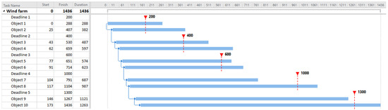
Figure 4.
Baseline schedule.
Construction tasks (activities of the Gantt chart) for each turbine are scheduled with unique start and finish dates, and each unit is subject to a predefined deadline for completion. In the baseline schedule, some of the units exceed their deadlines, incurring penalties accordingly. Such a situation results from preparation of the initial schedule without knowledge of the weather data specific for region of construction and contractual deadlines. A summary of the schedule and deadline data for each turbine is presented in Figure 4 and Table 2.
The calendar used in the project accounts for non-working days, including weekends and public holidays. The earliest project start date is set to 1 January 2026, and this marks day 0 in the scheduling model. Indirect costs amount to $8000 per day. Additional key financial parameters used in the simulation include the following:
- α = 10%,
- Pro = 40%,
- = 6%.
Each unit schedule consists of 10 activities (m = 10), namely:
- Surveying and land clearing.
- Access road construction.
- Foundation construction.
- Crane pad construction.
- Turbine installation p.I.
- Electrical network installation.
- Turbine installation p.II.
- Substation construction.
- Site rehabilitation.
- Turbine commissioning.
Detailed basic parameters (without weather impact) for activities are presented in Figure 5. The TP for the baseline schedule is equal to $−6,048,805, especially compared to the total cost of the project which is approximately $50 million.
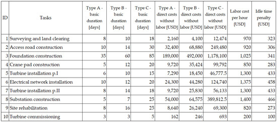
Figure 5.
Base task parameters.
The analyzed wind farm is located in northern Poland, in the area of the city of Koszalin. The form of the coefficients for construction works was adopted according to Table 3.
Table 3.
Weather productivity coefficients —formulae.
Based on the actual weather data for the location of the city of Koszalin downloaded from the https://www.ogimet.com website (index: 12105—KOSZALIN, POLAND; Latitude: 54-12-00 N; Longitude: 016-08-60 E; Altitude: 34 m, accessed on 1 July 2025), the values of RCCs were calculated, taking into account weather data from 2017 to 2024 for this location. The RCC values are calculated as the average values for the above year range and are given in Table 4. The values of the coefficients were calculated according to Table 3 and are presented in Table 5.
Table 4.
Raw Climatic Coefficients RCC for Koszalin according to weather data from 2017 to 2024.
Table 5.
Weather productivity coefficient values for case study activities.
The project described above serves as a case study for validating the performance of a scheduling and cash flow optimization model. The project’s complexity (stemming from multiple turbine types, different activity durations, deadline constraints, and financial implications) makes it a suitable benchmark for advanced construction planning methods.
The results obtained using the proposed method are presented below. Figure 6 shows the progression of the objective function during the optimization process, illustrating how the solution quality improved over iterations. Table 6 provides the permutation and parameters of the schedule optimized by the algorithm. Figure 7 compares the original (baseline) and improved (optimized) schedules. A slight improvement in the total duration was obtained as a side effect of the optimization process (from 1436 to 1411 days). The main advantages of the method can be seen when analyzing the improved cost parameters. The final value of the objective function after optimization is $1,042,082, a significant improvement over the original value of $−6,048,805. Most notably, the project was transformed from a loss-making operation into a profitable one.
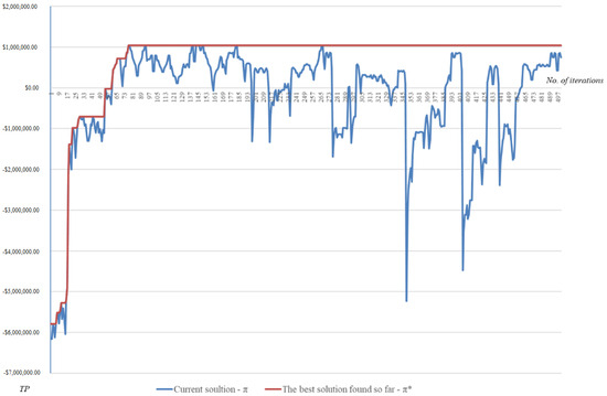
Figure 6.
The solution chart of the algorithm.
Table 6.
Optimized schedule—basic parameters.
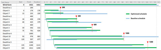
Figure 7.
Optimized vs. baseline schedule.
The initial project schedule was financially unfavorable due to its high sensitivity to weather-related risks, particularly prolonged periods of adverse wind conditions and precipitation, which disrupted critical construction activities and increased indirect costs. These weather-induced delays extended the project duration, triggered contractual penalties, and increased financing costs, ultimately leading to a projected negative cash flow. By applying the proposed scheduling and cash flow optimization method, the authors systematically integrated risk-resilient planning principles, enhancing the robustness of the schedule against such environmental uncertainties. The method reallocated weather-sensitive tasks to periods with statistically lower probabilities of unfavorable conditions, balanced resource utilization to reduce idle times, and incorporated financial constraints into the optimization process. As a result, the revised schedule not only shortened the overall project duration but, more importantly, mitigated the impact of weather-related delays on cash flow and cost accumulation. This improved resilience to risk transformed the project from a loss-making endeavor into a profitable one, demonstrating the practical value of incorporating robustness-oriented optimization into wind farm construction planning.
The application of the TS algorithm proved highly effective in addressing the scheduling problem. The dramatic improvement in the objective function highlights the algorithm’s ability to produce high-quality, cost-efficient solutions. This brings substantial benefits to the contractor, including reduced operational inefficiencies and more consistent service delivery. In the context of previous discussions, the results confirm that metaheuristic approaches like TS are powerful tools in complex planning tasks.
7. Discussion
This study proposed a scheduling model for multi-unit construction projects that includes the influence of weather events on work efficiency. The issue is critical for open-area construction projects like wind farms. By integrating historical weather data into the flow-shop framework, the model addresses an important gap in existing construction scheduling research. The approach also employs a comprehensive and practical objective function that considers direct costs, indirect costs, penalties, and potential financing requirements when cash flow becomes negative.
The numerical experiments illustrate the model’s robustness and practicality. In particular, the Tabu Search (TS) metaheuristic algorithm outperformed schedules generated by simpler algorithms, such as random search and climbing search, by a notable margin. For problem instances small enough for exhaustive evaluation (n = 6), the TS approach produced results that differed from the optimal solution by less than 1%. For more complex cases, it demonstrated strong performance, proving its applicability to large-scale projects where exhaustive methods are useless.
A case study of a wind farm construction project further underscores the method’s effectiveness and applicability to real-life problems. By analyzing a scenario of ten wind turbines plant, the TS algorithm successfully converted a project forecasted at a substantial financial loss ($−6,048,805) into a profitable outcome ($+1,042,082). This highlights the possible benefits of incorporating accurate weather-based productivity factors and advanced optimization procedures into project planning.
While the proposed method offers a powerful way to handle scheduling under dynamic weather conditions, a few limitations should be noted. First, the study relies on historical weather data, which may not account for rare or emerging climate extremes. Future work could integrate adaptive forecasting techniques or real-time sensor data to improve decision-making in rapidly changing conditions. Another possible improvement lies in exploring more complex contractual setups, such as multi-tier penalty structures or partnerships among multiple contractors. Future models could also consider variations in material delivery schedules, incorporating broader supply chain factors. That being said, using historical weather data for the productivity estimation is still far better than not taking such effects into consideration at all.
Overall, the proposed method offers a reliable and efficient way to handle multi-unit construction scheduling under variable conditions. Especially since renewable energy projects (like wind farms) are more and more popular all over the world. The approach described in the paper represents a significant step toward mitigating risks and enhancing profitability in complex construction ventures.
Author Contributions
Conceptualization, M.P., J.R. and B.S.; methodology, M.P., J.R. and B.S.; software, B.S.; validation, M.P. and J.R.; formal analysis, M.P.; investigation, M.P., J.R. and B.S.; resources, M.P., J.R. and B.S.; case study, J.R.; data curation, M.P.; writing—original draft preparation, M.P., J.R. and B.S.; writing—review and editing, M.P. and J.R.; visualization, J.R.; supervision, M.P., J.R. and B.S.; and project administration, M.P., J.R. and B.S. All authors have read and agreed to the published version of the manuscript.
Funding
This research received no external funding.
Data Availability Statement
Weather data for the location of the city of Koszalin was downloaded from the https://www.ogimet.com website (index: 12105—KOSZALIN, POLAND; Latitude: 54-12-00 N; Longitude: 016-08-60 E; Altitude: 34 m, accessed on 26 August 2025).
Acknowledgments
This research received no external support. The authors take full responsibility for the content of this publication.
Conflicts of Interest
The authors declare no conflicts of interest.
References
- Podolski, M.; Sroka, B. Cost optimization of multiunit construction projects using linear programming and metaheuristic-based simulated annealing algorithm. J. Civ. Eng. Manag. 2019, 25, 848–857. [Google Scholar] [CrossRef]
- Tomczak, M.; Jaśkowski, P. Harmonizing construction processes in repetitive construction projects with multiple buildings. Automat. Constr. 2022, 139, 104266. [Google Scholar] [CrossRef]
- Tomczak, M.; Jaśkowski, P. Customized particle swarm optimization for harmonizing multi-section construction projects. Automat. Constr. 2024, 162, 105359. [Google Scholar] [CrossRef]
- Sroka, B.; Rosłon, J.; Podolski, M.; Bożejko, W.; Burduk, A.; Wodecki, M. Profit optimization for multi-mode repetitive construction project with cash flows using metaheuristics. Arch. Civ. Mech. Eng. 2021, 21, 67. [Google Scholar] [CrossRef]
- Podolski, M.; Rosłon, J.; Sroka, B. The impact of the learning and forgetting effect on the cost of a multi-unit construction project with the use of the simulated annealing algorithm. Appl. Sci. 2022, 12, 12667. [Google Scholar] [CrossRef]
- Gupta, J.; Stafford, E.F., Jr. Flowshop scheduling research after five decades. Eur. J. Oper. Res. 2006, 169, 699–711. [Google Scholar] [CrossRef]
- Al Refaie, A.M.; Alashwal, A.M.; Abdul-Samad, Z.; Salleh, H. Weather and labor productivity in construction: A literature review and taxonomy of studies. Int. J. Product. Perform. Manag. 2021, 70, 941–957. [Google Scholar] [CrossRef]
- Ballesteros-Pérez, P.; Rojas-Céspedes, Y.A.; Hughes, W.; Kabiri, S.; Pellicer, E.; Mora-Melià, D.; del Campo-Hitschfeld, M.L. Weather-wise: A weather-aware planning tool for improving construction productivity and dealing with claims. Automat. Constr. 2017, 84, 81–95. [Google Scholar] [CrossRef]
- Moselhi, O.; Gong, D.; El-Rayes, K. Estimating weather impact on the duration of construction activities. Can. J. Civil. Eng. 1997, 24, 359–366. [Google Scholar] [CrossRef]
- Shahin, A.; AbouRizk, S.M.; Mohamed, Y.; Fernando, S. Simulation modeling of weather-sensitive tunnelling construction activities subject to cold weather. Can. J. Civil. Eng. 2014, 41, 48–55. [Google Scholar] [CrossRef]
- AACE® International. Schedule Levels of Detail-As Applied in Engineering, Procurement, and Construction; AACE® International Recommended Practice No. 37R-06; AACE® International: Fairmont, WV, USA, 2010. [Google Scholar]
- Guo, S.-J.; Chen, J.-H.; Chiu, C.-H. Fuzzy duration forecast model for wind turbine construction project subject to the impact of wind uncertainty. Autom. Constr. 2017, 81, 401–410. [Google Scholar] [CrossRef]
- Atef, D.; Osman, H.; Ibrahim, M.; Nassar, K. A Simulation-Based Planning System for Wind Turbine Construction. In Proceedings of the 2010 Winter Simulation Conference, Baltimore, MD, USA, 5–8 December 2010; pp. 3283–3294. [Google Scholar]
- Zhou, Y.; Miao, J.; Yan, B.; Zhang, Z. Stochastic resource-constrained project scheduling problem with time varying weather conditions and an improved estimation of distribution algorithm. Comput. Ind. Eng. 2021, 157, 107322. [Google Scholar] [CrossRef]
- Mohamed, E.; Jafari, P.; Chehouri, A.; AbouRizk, S. Simulation-Based Approach for Lookahead Scheduling of Onshore Wind Projects Subject to Weather Risk. Sustainability 2021, 13, 10060. [Google Scholar] [CrossRef]
- Podolski, M. Management of resources in multiunit construction projects with the use of a tabu search algorithm. J. Civ. Eng. Manag. 2017, 23, 263–272. [Google Scholar] [CrossRef]
- Rosłon, J.H.; Kulejewski, J.E. A hybrid approach for solving multi-mode resource-constrained project scheduling problem in construction. Open Eng. 2019, 9, 7–13. [Google Scholar] [CrossRef]
- AbouRizk, S.M.; Wales, R.J. Combined discrete-event/continuous simulation for project planning. J. Constr. Eng. Manag. ASCE 1997, 123, 11–20. [Google Scholar] [CrossRef]
- El-Rayes, K.; Moselhi, O. Impact of rainfall on the productivity of highway construction. J. Constr. Eng. Manag. ASCE 2001, 127, 125–131. [Google Scholar] [CrossRef]
- Carr, V.; Tah, J.H.M. A fuzzy approach to construction project risk assessment and analysis: Construction project risk management system. Adv. Eng. Softw. 2001, 32, 847–857. [Google Scholar] [CrossRef]
- Marzouk, M.; Hamdy, A. Quantifying weather impact on formwork shuttering and removal operation using system dynamics. KSCE J. Civ. Eng. 2013, 17, 620–626. [Google Scholar] [CrossRef]
- Golizadeh, H.; Sadeghifam, A.N.; Aadal, H.; Abd Majid, M.Z. Automated tool for predicting duration of construction activities in tropical countries. KSCE J. Civ. Eng. 2016, 20, 12–22. [Google Scholar] [CrossRef]
- Senouci, A.; Mubarak, S. Time-Profit Trade-Off of Construction Projects Under Extreme Weather Conditions. J. Constr. Eng. Project Manag. 2014, 4, 33–40. [Google Scholar] [CrossRef][Green Version]
- Senouci, A.; Mubarak, S. Multiobjective optimization model for scheduling of construction projects under extreme weather. J. Civ. Eng. Manag. 2016, 22, 373–381. [Google Scholar] [CrossRef]
- Senouci, A.; Al-Abbasi, M.; Eldin, N.N. Impact of weather conditions. Middle East J. Manag. 2018, 5, 34–49. [Google Scholar] [CrossRef]
- Galloway, P.D. Survey of the construction industry relative to the use of CPM scheduling for construction projects. J. Constr. Eng. Manag. ASCE 2006, 132, 697–711. [Google Scholar] [CrossRef]
- Arditi, D.; Tokdemir, O.B.; Suh, K. Challenges in line-of-balance scheduling. J. Constr. Eng. Manag. ASCE 2002, 128, 545–556. [Google Scholar] [CrossRef]
- Mattila, K.G.; Park, A. Comparison of linear scheduling model and repetitive scheduling method. J. Constr. Eng. Manag. ASCE 2003, 129, 56–64. [Google Scholar] [CrossRef]
- Rogalska, M.; Hejducki, Z. The application of time coupling methods in the engineering of construction projects. Tech. Trans. 2017, 114, 67–74. [Google Scholar] [CrossRef]
- Tomczak, M.; Jaśkowski, P. Scheduling repetitive construction projects: Structured literature review. J. Civ. Eng. Manag. 2022, 28, 422–442. [Google Scholar] [CrossRef]
- Bożejko, W.; Hejducki, Z.; Wodecki, M. Applying metaheuristic strategies in construction projects management. J. Civ. Eng. Manag. 2012, 18, 621–630. [Google Scholar] [CrossRef]
- Bożejko, W.; Hejducki, Z.; Wodecki, M. Flowshop scheduling of construction processes with uncertain parameters. Arch. Civ. Mech. Eng. 2019, 19, 194–204. [Google Scholar] [CrossRef]
- Anysz, H.; Buczkowski, B. The association analysis for risk evaluation of significant delay occurrence in the completion date of construction project. Int. J. Environ. Sci. Technol. 2019, 16, 5369–5374. [Google Scholar] [CrossRef]
- Assaad, R.; Abdul-Malak, M.A. Legal perspective on treatment of delay liquidated damages and penalty clauses by different jurisdictions: Comparative analysis. J. Leg. Aff. Disput. Resolut. Eng. Constr. 2022, 12, 04520013. [Google Scholar] [CrossRef]
- Graham, R.L.; Lawler, E.L.; Lenstra, J.K.; Kan, A.R. Optimization and approximation in deterministic sequencing and scheduling: A survey. Ann. Discrete Math. 1979, 5, 287–326. [Google Scholar] [CrossRef]
- Glover, F. Tabu search—Part I. ORSA J. Comput. 1989, 1, 190–206. [Google Scholar] [CrossRef]
- Glover, F. Tabu search—Part II. ORSA J. Comput. 1990, 2, 4–32. [Google Scholar] [CrossRef]
- Karamichailidou, D.; Kaloutsa, V.; Alexandridis, A. Wind turbine power curve modeling using radial basis function neural networks and tabu search. Renew. Energy 2021, 163, 2137–2152. [Google Scholar] [CrossRef]
- Ma, X.; Wang, Z.; Wang, C. An image encryption algorithm based on Tabu Search and hyperchaos. Int. J. Bifurc. Chaos. 2024, 34, 2450170. [Google Scholar] [CrossRef]
- Umam, M.S.; Mustafid, M.; Suryono, S. A hybrid genetic algorithm and tabu search for minimizing makespan in flow shop scheduling problem. J. King Saud Univ. Comput. Inf. Sci. 2022, 34, 7459–7467. [Google Scholar] [CrossRef]
- Bartz-Beielstein, T.; Chiarandini, M.; Paquete, L.; Preuss, M. Experimental Methods for the Analysis of Optimization Algorithms, 1st ed.; Springer: Berlin/Heidelberg, Germany, 2010. [Google Scholar] [CrossRef]
- Karnopp, D.C. Random Search Techniques for Optimization Problems. Automatica 1963, 1, 111–121. [Google Scholar] [CrossRef]
- Taillard, E. Some efficient heuristic methods for the flow shop sequencing problem. Eur. J. Oper. Res. 1990, 47, 65–74. [Google Scholar] [CrossRef]
- Kirkpatrick, S.; Gelatt, C.D.; Vecchi, M.P. Optimization by simulated annealing. Science 1983, 220, 671–680. [Google Scholar] [CrossRef]
- Ogbu, F.; Smith, D. The application of the simulated annealing algorithm to the solution of the n/m/Cmax flowshop problem. Comput. Oper. Res. 1990, 17, 243–253. [Google Scholar] [CrossRef]
- Lorenc, H. (Ed.) Atlas klimatu Polski (Eng. Polish Climate Atlas); IMGW: Warszawa, Poland, 2005. [Google Scholar]
- Kulejewski, J.; Ibadov, N.; Rosłon, J.; Zawistowski, J. Cash flow optimization for renewable energy construction projects with a new approach to critical chain scheduling. Energies 2021, 14, 5795. [Google Scholar] [CrossRef]
Disclaimer/Publisher’s Note: The statements, opinions and data contained in all publications are solely those of the individual author(s) and contributor(s) and not of MDPI and/or the editor(s). MDPI and/or the editor(s) disclaim responsibility for any injury to people or property resulting from any ideas, methods, instructions or products referred to in the content. |
© 2025 by the authors. Licensee MDPI, Basel, Switzerland. This article is an open access article distributed under the terms and conditions of the Creative Commons Attribution (CC BY) license (https://creativecommons.org/licenses/by/4.0/).