A Railway Mobile Terminal Malware Detection Method Based on SE-ResNet

Abstract

This paper proposes a residual network model integrated with an attention mechanism module for the detection and classification of malware on railway mobile terminals. To address the issues of insufficient and imbalanced samples, Wasserstein Generative Adversarial Networks (WGANs) are utilized to synthesize grayscale image data of malware with high similarity to real samples. The performance of the model is evaluated on the publicly available CIC-InvesAndMal2019 dataset and an extended balanced dataset. Experimental results demonstrate that the synergistic integration of residual networks, WGANs, and attention mechanisms significantly enhances the performance of the malware detection model. In the context of railway applications, the proposed approach also achieves favorable classification performance when applied to image datasets derived from malware samples of railway mobile terminals. Multiple ablation studies are conducted to individually validate the contributions of each technical component in improving the classification model’s efficacy. The adoption of the SE-ResNet architecture combined with WGAN-based data augmentation presents a practical and efficient technical solution.

1. Introduction

The application of railway mobile terminals has grown increasingly widespread in the railway industry, covering multiple aspects such as railway operations, maintenance, and inspection. During railway inspection operations, the use of mobile terminals assists railway staff in real-time data collection, recording, and processing, thereby enhancing operational efficiency. In the event of faults or accidents, multi-party voice and video calls enable remote command and coordinated handling, shortening the time required for fault resolution. In the locomotive system, these terminals facilitate the management of locomotive departure and arrival operations, allow real-time monitoring of crew activities, help prevent delays in addressing locomotive faults, and provide dispatchers with real-time locomotive location information to optimize scheduling management. Within the railway signaling system, GSM-R mobile terminals enable real-time voice communication among train drivers, station attendants, and dispatchers, ensuring the safety and efficiency of train operations. In passenger rail systems, voice and data communications via mobile terminals support passenger services, onboard ticket sales, and passenger transport management.

Currently, railway mobile terminals can be categorized into customized and general-purpose types, with Android-based systems being the dominant operating system. Due to the relatively high level of user permissions and flexibility inherent in the Android operating system, and within the context of a generalized and liberalized mobile application ecosystem, these terminals face significant threats from malicious software. These threats primarily include: 1. Adware: Generates revenue by displaying pop-up advertisements or installing unwanted applications on the device. 2. Ransomware: This type of malware encrypts files on the user’s device or locks the device, demanding a ransom for restoration. 3. Fake Security Software: Often disguises itself as system security software, deceiving users into believing their system is under illegal attack and misleading them into downloading paid software. 4. SMS Trojan Malware: Secretly subscribes to paid services by sending SMS messages without the user’s knowledge.

These threats pose significant risks to railway mobile applications and the stable operation of critical information infrastructure. In recent years, the railway industry has widely implemented regular cybersecurity inspection programs [1]. These initiatives involve identifying and addressing security threats and vulnerabilities within important information assets to reduce exposure and mitigate security risks. However, the detection of malware on railway mobile terminals has not yet been incorporated into the scope of routine cybersecurity inspections. Furthermore, annual activities such as classified protection assessments and risk evaluations have not included such checks within their frameworks. As a result, risks associated with railway mobile terminals remain outside the scope of daily monitoring and detection, leading to particularly prominent issues of unmanaged risks. If malware is installed, such software may masquerade as legitimate applications while performing malicious operations in the background. As mobile terminals serve as an extension of critical railway information infrastructure and important information systems, there is an urgent need to identify and detect malware on these devices to reduce the risk of attackers exploiting them to target internal railway systems.

2. Related Work

Malware detection is typically classified into two primary approaches: static feature analysis and dynamic feature analysis. Static analysis includes techniques such as signature scanning [2], signature-based scanning technology [3], and import table analysis [4]. Dynamic analysis encompasses heuristic scanning [5,6] and sandbox simulation technology [7,8,9].

Signature Scanning Technology involves extracting specific byte sequences (signatures) from malware as a basis for detection. These signatures can be strings, assembly instructions, or other distinctive features within the malware. During detection, file contents are scanned for sequences matching these signatures. The advantage of this method is its high scanning speed and a certain degree of broad detection capability, allowing it to identify various malware samples with similar characteristics. However, it may suffer from a relatively high false-positive rate.

Malware Signature Technology operates by extracting signatures from known malware and storing them in a signature database. Files or network traffic on a system are then scanned and compared against this database. A successful match indicates the potential presence of malware. The strength of this technique lies in its speed and efficiency for detecting known malware, typically resulting in a low false-positive rate. Its major limitation is its reliance on known signatures, making it ineffective against new malware or variants.

Import Table Analysis Technology involves analyzing the Import Table of Windows Portable Executable (PE) files to assess a program’s potential threat level. This technique is based on the program’s behavioral patterns rather than specific malware signatures. Its advantage is the ability to detect previously unknown threats. However, it also tends to have a higher false-positive rate because some legitimate programs may call API functions deemed “suspicious”.

Heuristic Scanning Technology, a form of dynamic analysis, improves the detection of unknown malicious programs by mitigating false negatives caused by binary file packing.

Sandbox Analysis Technology is another dynamic method where a suspect file is executed within a simulated, controlled virtual environment. Its behavior and function calls are monitored and analyzed to score its maliciousness.

The routine cybersecurity inspection work within the railway industry is a component of cybersecurity supervision. Inspectors are required to complete the collection of application software information from thousands of mobile terminals within a single inspection cycle. Dynamic analysis methods, which rely on analyzing software behavior such as network traffic, logs, and access patterns, are time-consuming and inefficient. They are unsuitable for the rapid collection of behavioral characteristics from a large number of mobile terminal applications within short time frames. While static analysis methods like malware signature technology offer high detection efficiency, their capability to detect variants or new code is very limited. Even minor changes, such as recompiling the file or altering a single byte, can cause the signature value to mismatch.

To address these limitations, this paper proposes a malware detection and identification method for mobile terminals based on WGAN and SE-ResNet. The main contributions are as follows:

(1)

Malware Parsing using Grayscale Images: Malware’s memory features are visualized by generating grayscale images, which aids in analyzing its behavioral patterns. Tools are used to extract memory data during malware execution, which is then converted into grayscale images (values 0–255). This visualization helps distinguish between different types of malware and, to some extent, mitigates the impact of code variants and obfuscation techniques employed by malware authors.

(2)

Malware Identification Method based on SE-ResNet: SE-ResNet, an improved version of ResNet that incorporates a squeeze-and-excitation attention mechanism module, is proposed. This module allows the network to adaptively recalibrate channel-wise feature responses, enhancing its robustness to varying tasks and input data. In tasks like image classification, SE-ResNet typically achieves higher accuracy than the original ResNet while maintaining low computational overhead.

(3)

Dataset Generation and Augmentation: To support model training, a malware dataset was constructed. The Canadian Institute for Cybersecurity—Investigation and Malware 2019 (CIC-InvesAndMal2019) dataset, captured in real-world environments and containing features like traffic, memory dumps, logs, permissions, and API calls, was used as the base dataset. Additionally, samples of railway mobile terminal malware were collected, and features such as traffic, memory, and logs were extracted in real environments, forming an extended railway malware sample set integrated into the repository.

(4)

Data Augmentation using WGANs: WGANs were employed for data augmentation. The WGAN generates synthetic grayscale image samples of malware to expand the training dataset. This enhances the scale and quality of the dataset, alleviating the current issues of insufficient samples and imbalanced distribution specific to railway mobile terminal malware, thereby improving the model’s generalization ability and detection accuracy.

3. Malware Detection Model

3.1. Overview

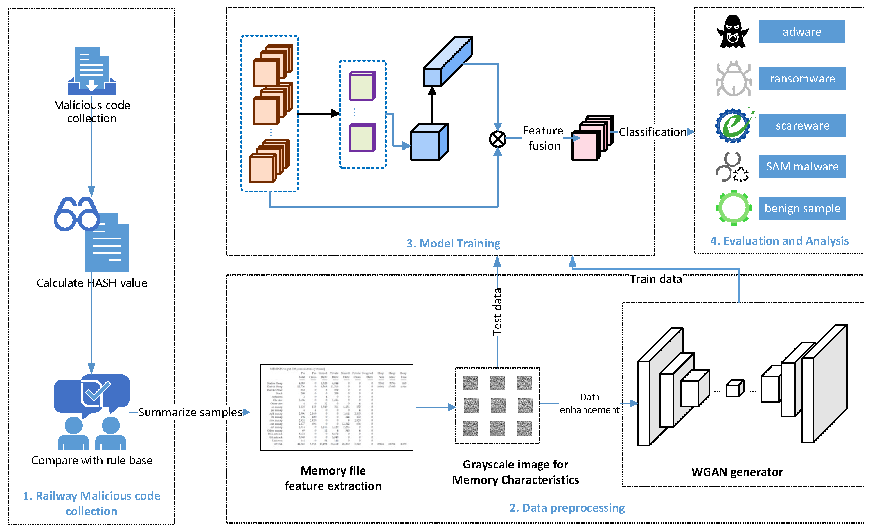
The overall architecture of the proposed method is illustrated in Figure 1. To construct the training set, validation set, and test set for the model, malware samples and benign software samples are integrated. The memory features of the samples are extracted and converted into grayscale images with a size of 28 × 28 pixels. WGANs are used to perform data augmentation on the malware samples, alleviating sample insufficiency and class imbalance, and mitigating overfitting issues in the classification model. The convolutional layers of the deep learning-based classification model are employed to extract features from the grayscale image samples, with important features being weighted. Through multi-level feature convolution, optimal training results are output. After multiple training iterations, a malware detection classification model for railway mobile terminals is obtained.

3.2. Classification Model

As a class of Convolutional Neural Network methods, Residual Neural Networks (ResNet) enable the network to better recognize and learn image features by transforming object characteristics into an image format [10,11,12,13]. Numerous research findings have demonstrated the outstanding performance of ResNet in image processing [14,15,16]. This transformation involves not only converting feature data into image pixel values but also includes normalizing the images to meet the input requirements of subsequent models. As an improved CNN model, ResNet does not suffer from vanishing gradients as the network depth increases. Furthermore, because the residual blocks in ResNet comprise convolutional layers for feature mapping, batch normalization, and Rectified Linear Unit activation functions, they facilitate skip connections that output optimal results, effectively preventing overfitting.

However, as network depth increases, features at different levels may possess varying degrees of importance. Traditional ResNet assigns equal weight to all feature channels or spatial locations, which may prevent the model from adequately focusing on critical information. To further enhance model performance, some researchers have introduced attention mechanisms into ResNet [17]. This enables the network to adaptively enhance important features and suppress irrelevant ones, thereby improving the model’s representational capacity and generalization performance.

This paper proposes incorporating a Squeeze-and-Excitation (SE) channel attention module after the residual blocks of the ResNet. The process first compresses spatial information through global average pooling, then learns channel weights via fully connected layers, dynamically adjusts the importance of each channel in the feature map, and finally recalibrates the features. The advantages of this classification model are mainly reflected in:

(1)

It enables the classification model to focus more effectively on useful features while suppressing less important ones, thereby enhancing feature representation capability.

(2)

Compared to the standard ResNet, it typically achieves higher accuracy in tasks such as image recognition and object detection.

(3)

The adoption of the SE module only marginally increases parameters and computational cost, yet significantly improves model performance. Additionally, the SE module can be flexibly embedded into each residual block of the ResNet without requiring extensive modifications to the original network architecture.

3.2.1. ResNet Model

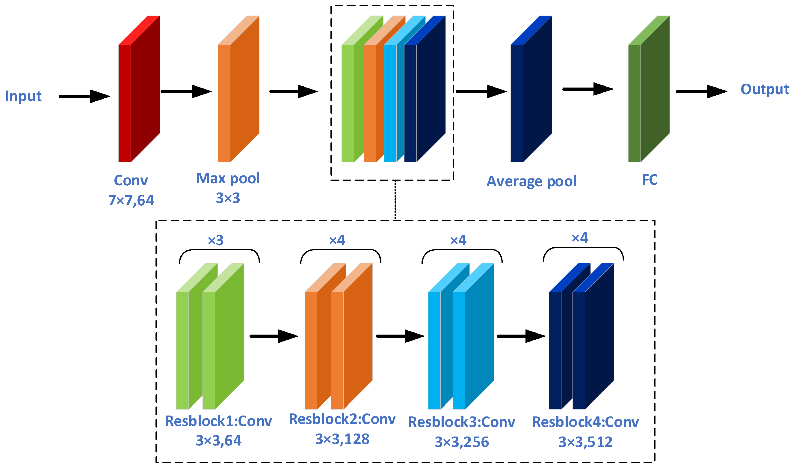
The ResNet34 network is a deep convolutional neural network model. Its architecture is depicted in Figure 2 [10], and the detailed structural diagram is presented in

Table 1. Detailed Network Architecture of ResNet34.

Layer	Size	Architecture
conv1	$16\times 16$	$7\times 7,64$
Resblock1	$8\times 8$	$3\times 3$ Max pool, stride 2
		$\left\{\begin{array}{l}3\times 3,64\\ 3\times 3,64\end{array}\right.\times 3$
Resblock2	$3\times 3$	$\left\{\begin{array}{l}3\times 3,128\\ 3\times 3,128\end{array}\right.\times 4$
Resblock3	$2\times 2$	$\left\{\begin{array}{l}3\times 3,256\\ 3\times 3,256\end{array}\right.\times 4$
Resblock4	$1\times 1$	$\left\{\begin{array}{l}3\times 3,512\\ 3\times 3,512\end{array}\right.\times 4$
output	$1\times 1$	Avg pool, flatten, softmax

. It sequentially consists of a 7 × 7 convolutional layer, a 3 × 3 pooling layer, 16 residual blocks (each containing two 3 × 3 convolutional layers), a global average pooling layer, and a fully connected layer. The reasons for selecting the ResNet34 network as the baseline model in this paper are twofold. On one hand, the size of the first convolutional layer (conv1) in ResNet34 is a 7 × 7 kernel. Compared to the more commonly used smaller-sized kernels, the 7 × 7 kernel offers a larger receptive field. This allows the network’s initial layer to more effectively capture larger-scale low-level feature patterns—such as edges and textures—in the input images. This characteristic is particularly suitable for classifying and identifying grayscale images of malware, which possess numerous detailed features, thereby providing a richer informational foundation for subsequent layers. On the other hand, the ResNet34 network requires relatively less computational resources and training time. Given that the applications installed on railway mobile terminals are relatively limited in variety and the devices generally have lower configurations, ResNet34, being a model with lower hardware requirements, is well-suited for this environment.

3.2.2. SE-ResNet Model

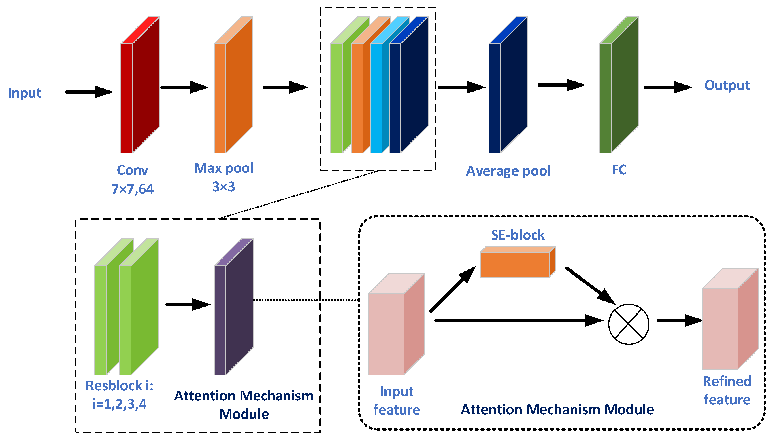
The SE-ResNet Model consists of 4 ResBlocks and 4 channel attention models, and it is shown in Figure 3.

Figure 4 illustrates the channel attention module within the SE-ResNet network. The module first applies a global average pooling operation to the input, obtaining a feature with dimensions [N, 1, 1, C], where N is the batch size and C is the number of channels. This is followed by two 1 × 1 convolutional operations that perform squeeze and excitation on the input. The output is then normalized using the Sigmoid function, retaining the original dimensions of [N, 1, 1, C]. Finally, the resulting output is multiplied element-wise with the original input to produce the final output of the SE-block module. This process can be expressed by the following formula:

$$channel\_weight=\mathrm{sigmoid}\left(\mathrm{conv}2(\mathrm{conv}1(\mathrm{avgpool}(x))\right)$$

(1)

$$SEblock\_output=x \times channel\_weight$$

(2)

$channel\_weight$ is the channel weight, $SEblock\_output$ is output. The complete SE-ResNet network architecture is detailed in

Table 2. SE-ResNet Network Parameter.

Layer	Size	Architecture
conv1	$16\times 16$	$7\times 7,64$
SE-block1	$16\times 16$	Avg pool $\mathit{conv}\left\{\begin{array}{l}1\times 1,4\\ 1\times 1,64\end{array}\right.$
Resblock1	$8\times 8$	$3\times 3$ Max pool, stride 2
		$\left\{\begin{array}{l}3\times 3,64\\ 3\times 3,64\end{array}\right.\times 3$
SE-block2	$8\times 8$	Avg pool $\mathit{conv}\left\{\begin{array}{l}1\times 1,4\\ 1\times 1,64\end{array}\right.$
Resblock2	$3\times 3$	$\left\{\begin{array}{l}3\times 3,128\\ 3\times 3,128\end{array}\right.\times 4$
SE-block3	$4\times 4$	Avg pool $\mathit{conv}\left\{\begin{array}{l}1\times 1,4\\ 1\times 1,64\end{array}\right.$
Resblock3	$2\times 2$	$\left\{\begin{array}{l}3\times 3,256\\ 3\times 3,256\end{array}\right.\times 4$
SE-block4	$2\times 2$	Avg pool $\mathit{conv}\left\{\begin{array}{l}1\times 1,4\\ 1\times 1,64\end{array}\right.$
Resblock4	$1\times 1$	$\left\{\begin{array}{l}3\times 3,512\\ 3\times 3,512\end{array}\right.\times 4$
output	$1\times 1$	Avg pool, flatten, softmax

. The network primarily consists of 4 ResBlocks and 4 SE-Blocks. Specifically, the structure of the 4 ResBlock modules has been fine-tuned to align with the requirements of this classification task.

3.3. Wasserstein Generative Adversarial Network (WGAN)

In 2014, Goodfellow et al. proposed Generative Adversarial Networks (GANs) [18], which have since been widely applied across various domains such as image super-resolution reconstruction [19], object detection [20], and text generation [21]. GANs primarily address the problem of approximating probability distributions by optimizing model parameters through adversarial interactions between two networks, thereby circumventing the need for Markov chains to estimate likelihood functions. However, GANs also suffer from non-negligible limitations, including poor training stability and susceptibility to mode collapse. To address these issues, Arjovsky et al. proposed the Wasserstein Generative Adversarial Network (WGAN) [22]. WGAN replaces the Jensen-Shannon (JS) divergence with the Wasserstein distance to measure the discrepancy between the generated and real data distributions, effectively mitigating training instability caused by vanishing gradients [23]. A schematic diagram of the WGAN architecture is shown in Figure 5.

Similar to traditional GANs, the WGAN framework comprises two core components: a Generator and a Discriminator (also referred to as a “Critic” in WGAN terminology). These two components engage in a more robust adversarial game. The primary objective of the Generator remains consistent with the original GAN—to learn the distribution of the real data. It takes a random noise vector as input and, through the transformation of neural network layers, ultimately outputs a synthetic data sample that closely approximates the real data distribution.

The WGAN introduces critical improvements to the traditional GAN in both architecture and objective function, with its core distinction lying in the transformed role and training objective of the discriminator. In WGAN, the discriminator (commonly termed the “Critic”) no longer performs binary classification but instead learns a function that outputs an unbounded real-valued score for input samples. This score can be interpreted as an estimator of the Wasserstein distance between the generated and real data distributions. During training, the Critic strives to assign higher scores to real samples and lower scores to generated ones, thereby attempting to maximize this estimated distance. Conversely, the Generator optimizes its parameters to enhance the quality of its generated samples to achieve higher scores from the Critic, consequently minimizing the distance. This adversarial mechanism, centered on optimizing the Wasserstein distance, effectively mitigates common issues in traditional GAN training, such as vanishing gradients and mode collapse. It results in a more stable training process, and the Critic’s output scores themselves can serve as an intuitive indicator of training progress and generation quality.

The loss function of WGAN generator is as follows:

$$l_G=-D(G(z))$$

(3)

In the formula, $z$ is the random noise vector input to the generator, $G(z)$ denotes the synthetic data output by the generator, and $D\left(G(z)\right)$ refers to the critic function. This loss function directly encourages the generator to produce samples that receive high scores from the critic.

The loss function for the discriminator (critic) is expressed as follows:

$$l_{\mathrm{D}}=D(G(z))-D(x)$$

(4)

In the above formula, $x$ represents samples drawn from the real data distribution. It is important to note that the objective of the Critic is to minimize $l_{\mathrm{D}}$, thereby widening the score disparity between real and generated samples. To satisfy the Lipschitz continuity constraint required for the computation of the Wasserstein distance, our model adheres to the original WGAN design by employing a weight clipping strategy to restrict the parameters of the Critic.

In recent years, GANs and their improved variants have been increasingly applied in the field of malware data augmentation. Literature [24] proposed a classification method that enhances model family attribution capability by creating a dataset of malware variants. This method employs an improved generative adversarial network for malware classification, utilizing Ghost modules and Dropout layers to balance the adversarial capabilities of the generator and discriminator. The proposed model achieves stronger feature extraction capability, reduced resource consumption, and faster inference speed, meeting the demands for anti-obfuscation capability and high generalization in contemporary malware classification models given the rapid evolution of malware. To address the issue of poor machine learning classification performance caused by imbalanced network traffic datasets, Literature [25] introduced generative adversarial networks and designed a multi-class evasion generative adversarial network. This approach tackles the imbalanced dataset problem encountered when using machine learning methods for classification detection. This data augmentation method can not only generate adversarial samples but also utilize the trained discriminator as a classifier for the dataset. Literature [26] compared generative adversarial networks with variational autoencoders, experimentally demonstrating that GAN models are more effective than variational autoencoders for generating malware data and more conducive to improving detection accuracy. In the experiments presented in this paper, WGAN will also be employed as a data augmentation technique for the original sample set.

In the subsequent experiments of this study, we opted for the WGAN with weight clipping instead of the more stable WGAN-GP (Wasserstein Generative Adversarial Network—Gradient Penalty), primarily because WGAN-GP requires the computation of gradient norms on interpolated samples, which increases computational complexity. Given that this task processes low-resolution 28 × 28 grayscale images, the original WGAN is already capable of effective convergence. Furthermore, weight clipping offers a more streamlined implementation, avoiding the burden of tuning hyperparameters such as the gradient penalty coefficient λ, thereby better facilitating the reproducibility and efficiency of the research.

4. Simulation Experiments

The simulation is divided into three phases: Data processing, Model training and Performances evaluation, which is shown in Figure 6.

4.1. Data Processing Phase

4.1.1. Dataset Establishment

Regarding dataset selection, the CIC-InvesAndMal2019 dataset was adopted as the original dataset. This dataset originates from real software samples collected by software memory collectors installed on 5000 real devices, which accurately reflects the attack scenarios on network equipment. The dataset comprises 426 malware samples and 5065 benign software samples. The categories of malware families contained in the dataset are presented in

Table 3. Types of Malware in the Dataset.

Malware	Malware Families	Malware	Malware Families
adware	Dowgin	ransomware	Charger
	Ewind		Jisut
	Feiwo		Koler
	Gooligan		LockerPin
	Kemoge		Simplocker
	koodous		Pletor
	Mobidash		PornDroid
	Selfmite		RansomBO
	Shuanet		Svpeng
	Youmi		WannaLocker
scareware	AndroidDefender	SMS Malware	BeanBot
	AndroidSpy		Biige
	AV for Android		FakeInst
	AVpass		FakeMart
	FakeApp		FakeNotify
	FakeApp.AL		Jifake
	FakeAV		Mazarbot
	FakeJobOffer		Nandrobox
	FakeTaoBao		Plankton
	Penetho		SMSsniffer
	VirusShield		Zsone

.

Since benign samples accounted for over 90% of the original CIC-InvesAndMal2019 dataset, stratified random sampling was employed to more effectively learn the characteristic patterns of malware, prevent the model from being dominated by the majority class (benign samples), and ensure the data quality and representativeness of each malware subset. Specifically, approximately 614 samples were randomly selected from the original benign samples, and about 410 samples were randomly chosen from the original malware samples. These were combined to form a preliminary balanced dataset containing 1024 samples, with malware representing approximately 40% of the total. During the selection of benign samples, diverse Android application types—such as browsers, office software, and multimedia tools—were incorporated to enhance sample diversity.

4.1.2. Data Preprocessing

Based on the investigation of malware behavioral patterns, different categories of malware demonstrate distinct behavioral characteristics:

Adware is characterized by frequent network connections to retrieve and display advertisements, resulting in abnormal system resource consumption. Verification methodology primarily involves monitoring network traffic for anomalous connections to known advertising domains, or examining system logs for non-user-triggered interface pop-up events. Ransomware operates by persistently scanning and encrypting user files. Verification can be achieved by detecting sequences of API calls associated with encryption algorithms within processes. Fake Security Software functions by intimidating users through fabricated security alerts and guiding them to install additional software. Verification involves analyzing system notification logs to identify counterfeit warnings containing keywords such as “virus,” “infected,” or “repair immediately. “SMS Malware demonstrates behaviors including abuse of SMS transmission permissions and unauthorized collection of contact information. Verification methods include examining SMS transmission logs to confirm the presence of unsolicited messages sent to specific numbers. For empirical validation, this study selected 50 samples from each of the aforementioned four malware categories. The effectiveness analysis revealed that 49 Adware samples, 48 Ransomware samples, 47 Fake Security Software samples, and 46 SMS Malware samples successfully triggered their expected malicious behaviors, yielding effectiveness rates exceeding 90% across all categories. These results confirm the suitability of the sample set for providing training and testing data in subsequent experimental phases.

This study captures volatile memory from Android devices and Linux systems by executing malware samples in real-world environments using the Loadable Kernel Module (LiME)—Linux Memory Extractor. As LiME operates as a kernel module that must be loaded into the system kernel space, its usage consequently requires obtaining root privileges on the target device. In practical operation, memory images can be acquired through two modes: direct writing to local storage or transmission over a network to a remote server. These requirements determine that LiME is primarily suitable for testing environments where administrative control has been established. LiME enables comprehensive capture of all memory contents on Android devices, thereby minimizing interactions between user space and kernel space during memory extraction. To reduce data storage requirements, this study extracts individual process memory rather than the entire system memory. The memory feature extraction workflow is illustrated in Figure 7.

(1) Process Selection: Fundamental processes were selected based on the behavioral objectives of different malware categories. This involved investigating the common manifestations of various malware types in terms of process activity. During the screening process, care was taken to ensure that the execution of each sample included the selected processes. Based on the analysis of malware behaviors, this study selected a number of fundamental system processes and application processes with high prevalence, as detailed in

Table 4. Selected Process for Feature Extraction.

No.	Name	Description
1	com.android.chrome	Chrome Browser
2	com.google.android.gms	Google Application and API
3	com.google.process.gapps	Google Software Service
4	android.process.media	Android Media Storage System Process
5	xyz.klinker.messenger	Pulse Application (Communication)
6	com.facebook.katana	Facebook Application
7	com.google.android.inputmethod.latin	Google Input
8	com.android.phone	Package Name of the System Telephony Application on Android Devices
9	com.android.nfc	NFC (Near Field Communication)
10	com.google.android.googlequicksearchbox:interactor	Google Search Box
11	com.android.systemui	Android System UI
12	system	Core System Processes

.

Different malware families lead to anomalous behaviors across distinct processes. The 12 processes listed in Table 4 constitute a minimal sufficient set designed to ensure comprehensive detection coverage. This selection achieves coverage of the system’s primary functional layers, including the system core (system), user interface (systemui), network communication (chrome, gms), underlying services (phone, nfc), and typical user applications. Collectively, they form a mutually complementary set of information that effectively characterizes the system’s global state.

(2) Feature Extraction: The specific memory features are extracted from all samples and denoted as $R=\{P_1,P_2,\cdots ,P_{12},L\}$, $P_i$ represents the process, $i\in (1,12)$, $P_i=\{f_1,f_2,\cdots ,f_n\}$, $f_j$ presents the specific memory feature, $j\in (1,65)$, $L$ represents the sample labels, and $L$$\in${(0: Benign), (1: adware), (2: ransomware), (3: Scareware), (4: SMS Malware)}. This paper takes the com.android.systemui process as an example to elucidate the specific definitions of each category of memory features collected in our study. The feature set of this process comprehensively represents the feature template employed for all analyzed processes. Each memory feature corresponds to multiple parameters, encompassing PSS, Private Dirty, Shared Clean, among others. The memory features of a typical process are detailed in

Table 5. Memory Feature Description.

Memory Feature	Description
Native Heap	Memory allocated via malloc in Native Code
Dalvik Heap	Space allocated by the Dalvik Virtual Machine (excluding its own overhead)
Dalvik Other	Memory occupied by class data structures and indices
Stack	Stack memory
Cursor	Space occupied by CursorWindow (SQL-related)
Ashmem	Anonymous Shared Memory (ASHMem)
Other dev	Memory occupied by internal drivers
.so mmap	Memory occupied by mapped .so code
.jar mmap	Memory occupied by Java file code
.apk mmap	Memory occupied by APK code
.ttf mmap	Memory occupied by TTF file code
.dex mmap	Memory occupied by mapped .dex code
Other mmap	Memory occupied by other files

.

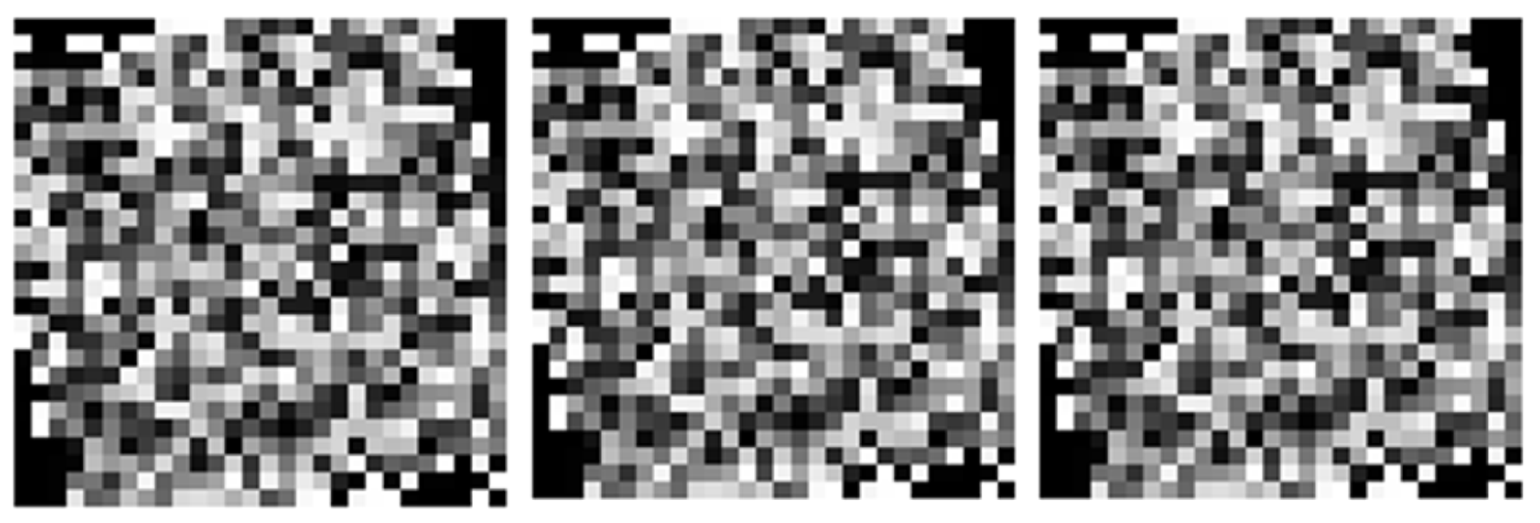
(3) Feature Processing: First, features are read from the CSV file following a column-wise order, where the first column corresponds to feature vector index 0, the second column to index 1, and so forth, up to the 784th column. For each dimension in the final 784-dimensional vector, min-max normalization is applied per feature, constraining the normalized values to the range [0, 1]. Subsequently, the 784-dimensional vector is reshaped following a row-major order: the first 28 values form the first row of the image, the next 28 values form the second row, and this continues until the last 28 values constitute the 28th row. Finally, the dataset is transformed into 784-dimensional data, which is then converted into 28 × 28 grayscale images (as shown in Figure 8) using an image conversion algorithm (detailed in

Table 6. Pseudocode for Converting Memory Features into Images.

Input	CsvFile
Output	ImageFile normalize the CsvFile for each row ∈ CsvFile transform row into two-dimensional matrix save matrix as grayscale insert grayscale into ImageFile end return ImageFile

). This results in a 28 × 28 two-dimensional matrix where each value falls within the range [0, 255].

The rationale for adopting the lower 28 × 28 resolution is twofold. First, this resolution demands fewer model parameters and lower computational complexity, enabling faster training and inference of the classification model and facilitating deployment in resource-constrained environments. Second, 28 × 28 grayscale images are sufficient to capture the essential memory features and their associated parameters.

4.1.3. Data Augmentation

Training Data Scale and Quality as Determinants of Model Performance: The scale and quality of training data are pivotal factors determining model performance. Training models on limited datasets can easily lead to overfitting and weaken their generalization capability. Constrained by the conditions for memory feature acquisition, the original malware sample set constructed in this study is limited in scale, with samples specific to the railway mobile terminal scenario being particularly scarce. To mitigate the constraints imposed by data insufficiency on model performance and to enhance the robustness and generalization capability of the classifier, this study employs the Wasserstein Generative Adversarial Network (WGAN) proposed in Section 3.3 to synthesize and augment grayscale image samples corresponding to various categories of malware, thereby achieving effective data augmentation.

(1)

Training Process

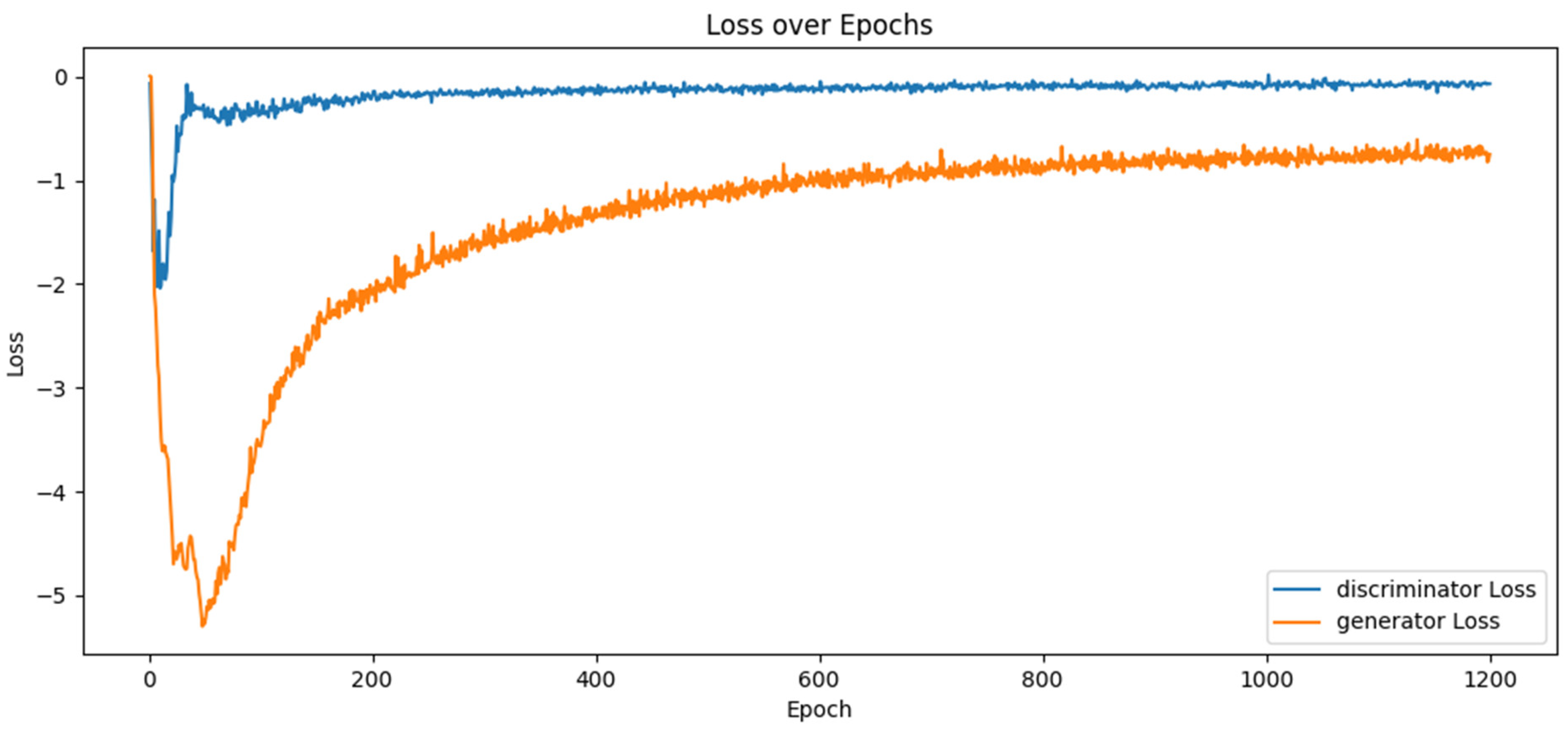
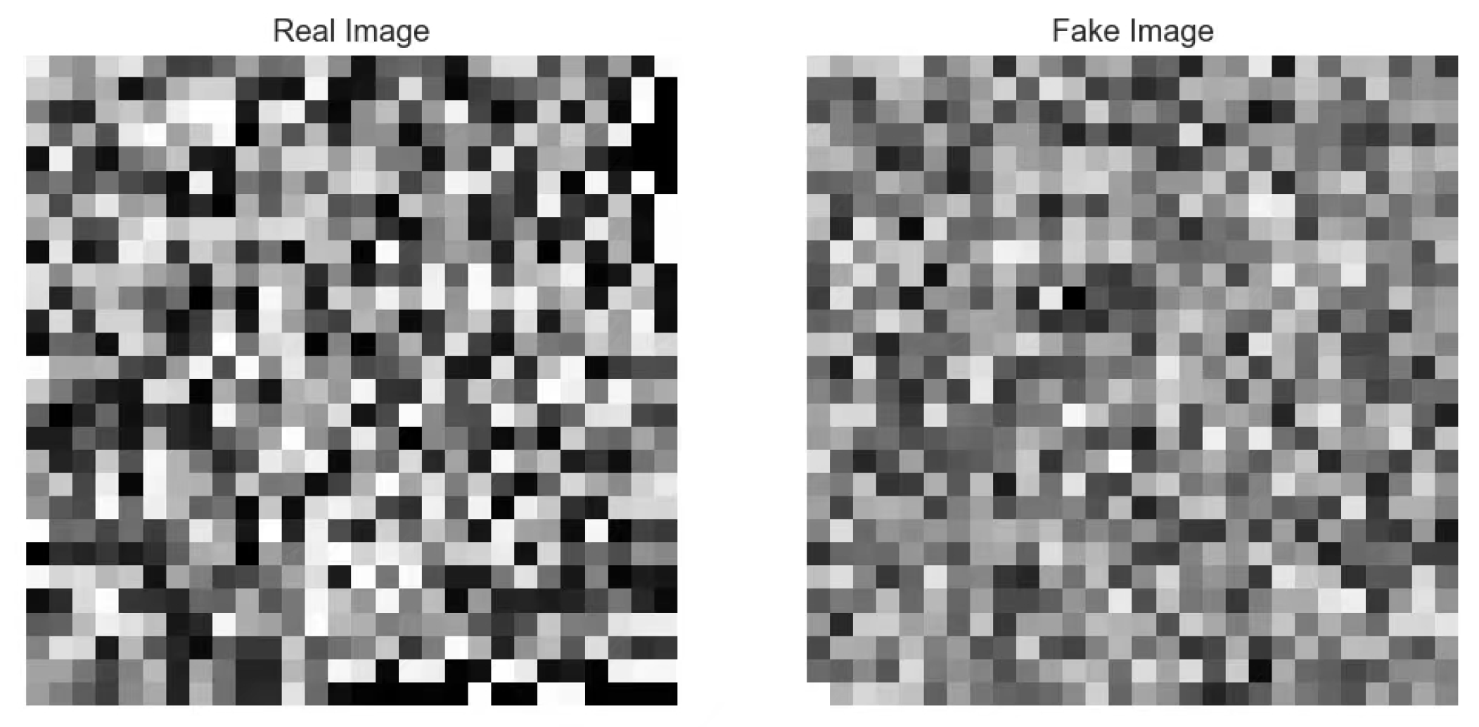
To illustrate the training dynamics and generation effectiveness, Figure 7 depicts the changes in the loss functions of both the generator and the discriminator throughout the training process, reflecting the convergent trend of the model training. Figure 9 presents the output of the generator given random noise inputs during the early stages of training, where the generated content lacks effective structure. In contrast, Figure 10 and Figure 11 shows samples generated after 1200 training epochs; these exhibit clear image characteristics and are visually highly similar to real malware grayscale images. This indicates that the WGAN has successfully learned to approximate the original data distribution, thereby providing high-quality augmented data for subsequent classification tasks.

(2)

Quality Assessment of Synthetic Data

To quantitatively evaluate the quality and diversity of the samples generated by the WGAN, we computed the FID (Fréchet Inception Distance) score between the synthetic images and the real training images for each category. The FID score measures the distributional discrepancy between two image datasets by comparing the mean and covariance of features extracted from an intermediate layer of a pre-trained Inception-v3 neural network. A lower FID score indicates a closer match between the distribution of the generated data and that of the real data, signifying higher generation quality. The FID scores for the samples generated in each category in this study are as follows: Adware 15.2, Ransomware 21.7, Fake Security Software 16.9, and SMS Malware 19.3. The FID scores for all four malware categories are below 25, which represents a relatively ideal outcome. Our results demonstrate that the WGAN successfully learned the underlying distribution of the real data and generated synthetic data that closely resembles the real samples in both visual and statistical characteristics. This indicates that the WGAN generator in this work is capable of producing high-quality, highly diverse, and category-consistent new samples, thereby fulfilling the requirements for data augmentation.

(3)

Hyperparameter Configuration

The main parameter settings for the WGAN in our experiments are as follows:

• Generator: A 100-dimensional latent vector serves as the input. The network consists of four hidden layers with neuron counts of 128, 256, 512, and 1024, respectively. Each hidden layer is followed by Batch Normalization and a LeakyReLU activation function. The output layer employs a Tanh activation function to generate 28 × 28 pixel grayscale images.
• Discriminator (Critic): The discriminator is a three-layer fully connected network with neuron counts of 512, 256, and 1, sequentially. Hidden layers use the LeakyReLU activation function. The output layer does not use a Sigmoid function; instead, it directly outputs a real-valued score to estimate the Wasserstein distance between the input sample and the real data distribution.
• Training Configuration: The RMSProp optimizer is employed with a learning rate set to 5 × 10⁻⁵ and a batch size of 16. To enforce the Lipschitz constraint required by the WGAN framework, discriminator weights are clipped to the range [−0.01, 0.01] to stabilize the training process.

The algorithmic procedure for generating image samples using the GAN is presented in

Table 7. Image Generation with WGAN.

Input	Real Image Dataset and Random Noise
Output	for real_images in data_loader: Train discriminator Generate noise vector z Generate fake_images = G(z) Calculate discriminator loss on real and fake images Update discriminator parameters Clip discriminator parameters Train generator Regenerate fake_images Calculate generator loss update generator parameters Output training progress and generated samples

.

To preserve the authentic data distribution during testing, the training set and test set were partitioned according to the class proportions. Observation of the data ratios reveals a severe imbalance between the number of malware samples in certain classes and the benign samples, which constitute the majority class. Therefore, this study employs the WGAN algorithm to augment the number of samples for each rare type in the original dataset to 600 individually. As shown in

Table 8. Sample Number Setting.

Malware	Number of Original Sample	Number of Sample Generated from WGAN	Number of Sample After Augmentation
adware	103	497	600
ransomware	97	503	600
scareware	105	495	600
SAM malware	105	495	600
benign	614	0	614

, the overall class distribution of the dataset becomes relatively balanced after data augmentation. A separate WGAN model is trained for each malware category to generate an independent dataset, ensuring that the generated samples are assigned explicit malware class labels.

4.2. Model Training Stage

Experimental Hardware Environment: The experiments in this study were conducted on a Windows 11 operating system, utilizing an Intel I9-12900K CPU, 32 GB of RAM, an NVIDIA A2000 GPU, and the PyTorch 2.4.1 deep learning library.

Test Set Partitioning: From the complete set of real samples, a subset (20%) of real samples was first randomly partitioned to form an independent test set. This set exclusively contained real samples, with no samples generated by the WGAN. This set was strictly isolated, and its sole purpose was to provide a single, unbiased performance evaluation simulating a real-world application scenario.

Training-Validation Set Partition: This study employs K-fold cross-validation to construct the training-validation sets, which collectively serve for model development and parameter tuning. The training-validation dataset is randomly partitioned into K similarly sized subsets. In each fold iteration, one of these subsets is designated as the Validation Set, while the remaining K-1 subsets constitute the Training Set. Specifically, in this experiment, K = 5.

The distribution of samples in the training-test dataset is detailed in

Table 9. Training-Validation Sampling Set.

Malware Families	Sample Number of Training-Validation in Original Dataset	Sample Number of Training-Validation After Augmentation	Test Sample Number with 20% of Original Dataset
adware	82	600	21
ransomware	77	600	20
scareware	84	600	21
SAM malware	84	600	21
benign	492	614	122

. To prevent data leakage, the data augmentation process is performed independently within each fold: during each fold, only the genuine samples from the designated training set (constituting 64% of the original data) within that fold are utilized to train the WGAN. Using the trained WGAN, we perform sampling exclusively on the samples within that fold’s training set, augmenting the number of samples for each malware category to 600. The validation set within that fold (constituting 16% of the original data) does not participate in the augmentation and is solely used for model selection during that particular training round.

4.3. Evaluation and Analysis Stage

During the evaluation and analysis stage, this study conducted comparative experiments using both the ResNet and SE-ResNet models to assess performance before and after dataset augmentation. The performance of these two model types was compared and analyzed. Evaluation metrics included Precision, F1-score, Recall, and accuracy, whose expressions are given as follows:

$$\mathrm{precision}={\displaystyle \frac{TP}{TP+FP}}$$

(5)

$$\mathrm{recall}={\displaystyle \frac{TP}{TP+FN}}$$

(6)

$$\mathrm{F}1\text{-}\mathrm{score}={\displaystyle \frac{2\times \mathrm{precision}\times \mathrm{recall}}{\mathrm{precision}+\mathrm{recall}}}$$

(7)

$$\mathrm{accuracy}={\displaystyle \frac{TP+TN}{TP+TN+FP+FN}}$$

(8)

In the expressions above,

• $TP$: Number of positive samples correctly predicted as positive.
• $TN$: Number of negative samples correctly predicted as negative.
• $FP$: Number of negative samples incorrectly predicted as positive.
• $FN$: Number of positive samples incorrectly predicted as negative.

4.3.1. ResNet Model

ResNet model adopted in this study utilizes the ResNet-34 architecture, as detailed in Section 3.2.1. The Adam optimizer was used with a learning rate (lr) of 0.0001, a batch size of 64, a weight decay of 1 × 10⁻⁵, and the model was trained for 100 epochs. All experiments were conducted using a random seed of 42 (this seed value remains consistent for all subsequent experiments). To ensure the model achieves optimal generalization performance and effectively avoids overfitting, this experiment employed an early stopping strategy based on validation loss during the training process. Specifically, the patience value was set to 20 epochs; training was automatically terminated if the validation loss failed to decrease for 20 consecutive epochs. Throughout the training process, the model checkpoint with the lowest validation loss was continuously saved. The performance evaluation on the test set was consistently conducted using this optimal checkpoint model, thereby ensuring the reliability of the results. The test dataset used for the evaluation is presented in Table 9.

Table 10. Comparison of Classification Results.

Type	Original Dataset			Augmented Dataset
	Precision	Recall	F1-Score	Precision	Recall	F1-Score
benign	0.973	0.978	0.976	0.979	1.000	0.989
adware	0.773	0.567	0.654	0.818	0.600	0.692
ransomware	0.500	0.655	0.567	0.957	0.759	0.846
scareware	0.488	0.645	0.556	0.638	0.968	0.769
SMS Malware	0.895	0.548	0.680	0.920	0.742	0.821
average	0.726	0.679	0.686	0.862	0.814	0.824

presents the experimental results based on the ResNet classification model. The results indicate that in the initial experiment, the average F1-score and Precision were 0.686 and 0.726, respectively. After expanding the dataset with grayscale images generated by the WGAN, the F1-score and Precision increased to 0.824 and 0.862, representing a 20% improvement in the F1-score and an 18.84% increase in Precision. These experimental results demonstrate a significant enhancement in the classification performance of the algorithm after data augmentation. Notably, the classification Precision for ransomware and SMS malware samples reached 95.65% and 92%, respectively, while their F1-scores improved to 0.846 and 0.821.

4.3.2. SE-ResNet Model

The network architecture of the SE-ResNet classification model used in this study refers to Section 3.2.2. The Adam optimizer was employed with a learning rate (lr) of 0.0001, a first-moment decay rate (β1) of 0.900, a second-moment decay rate (β2) of 0.999, a batch size of 64, a weight decay of 1 × 10⁻⁵, and the model was trained for 600 epochs. In this experiment, an early stopping strategy based on validation loss was implemented during the training process, with specific parameters consistent with those described in Section 4.3.1. The test dataset used for evaluation is presented in Table 9.

Table 11. Comparison of Classification Results.

Type	Original Dataset			Augmented Dataset
	Precision	Recall	F1-Score	Precision	Recall	F1-Score
benign	0.989	1.000	0.995	0.968	1.000	0.984
adware	0.516	0.533	0.525	0.609	0.933	0.737
ransomware	0.900	0.931	0.915	1.000	0.897	0.946
scareware	0.613	0.613	0.613	0.957	0.710	0.815
SMSMalware	0.926	0.807	0.862	1.000	0.645	0.784
average	0.789	0.777	0.782	0.907	0.837	0.853

presents the experimental results of the SE-ResNet classification model. The results show that in the initial experiment, the average F1-score and Precision were 0.782 and 0.789, respectively. After augmenting the dataset with grayscale images generated by the WGAN, the F1-score and Precision increased to 0.853 and 0.907, representing a 9% improvement in F1-score and an increase of 14.95% in Precision. Furthermore, the classification Precision for adware and ransomware samples reached 60.86% and 100%, respectively, while their F1-scores improved to 0.737 and 0.946. The experimental results indicate that the classification performance of the model was significantly optimized after data augmentation.

As can be observed from the experimental results presented in Table 10 and Table 11, the utilization of WGAN-generated grayscale images for data expansion effectively mitigates issues of data insufficiency and imbalance. This approach achieves data augmentation and significantly enhances the model’s performance in malware classification.

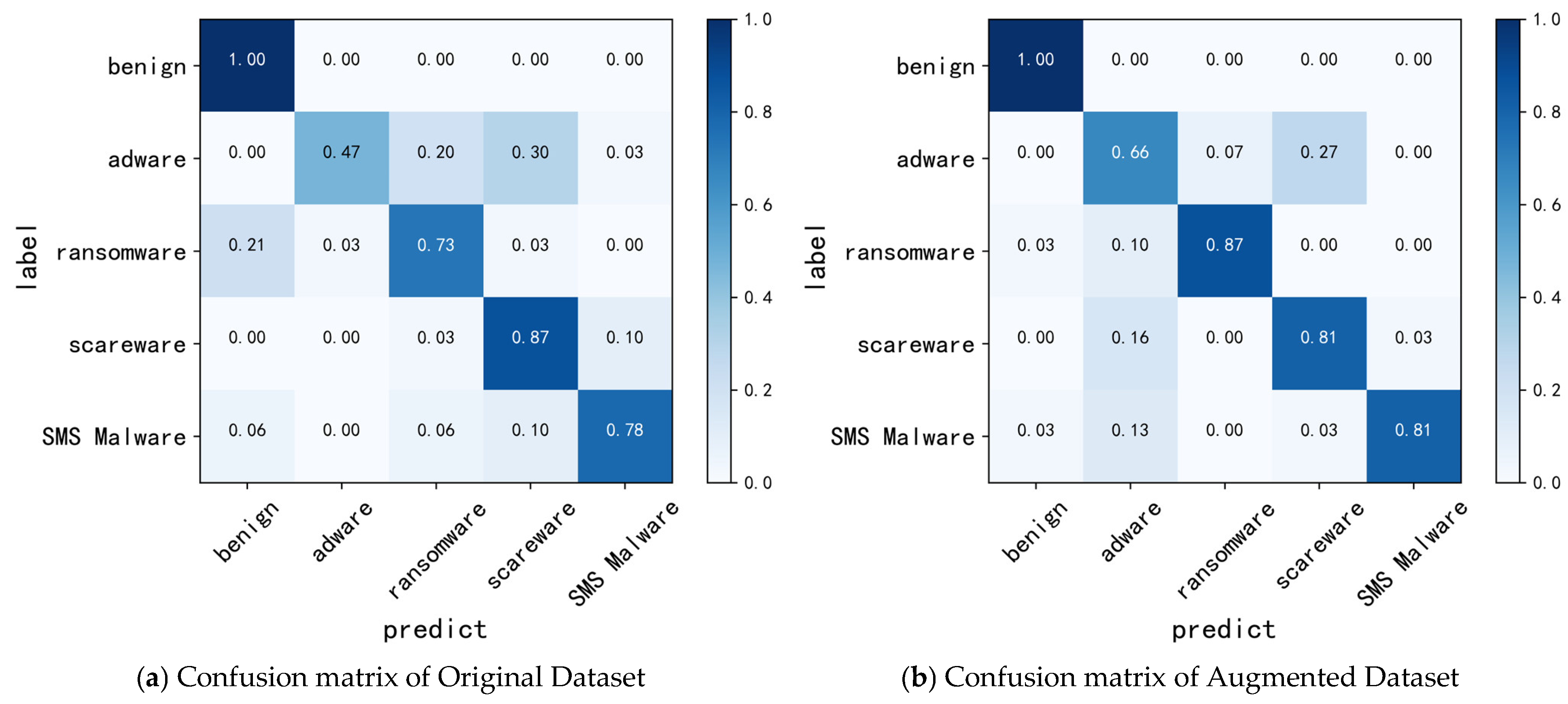
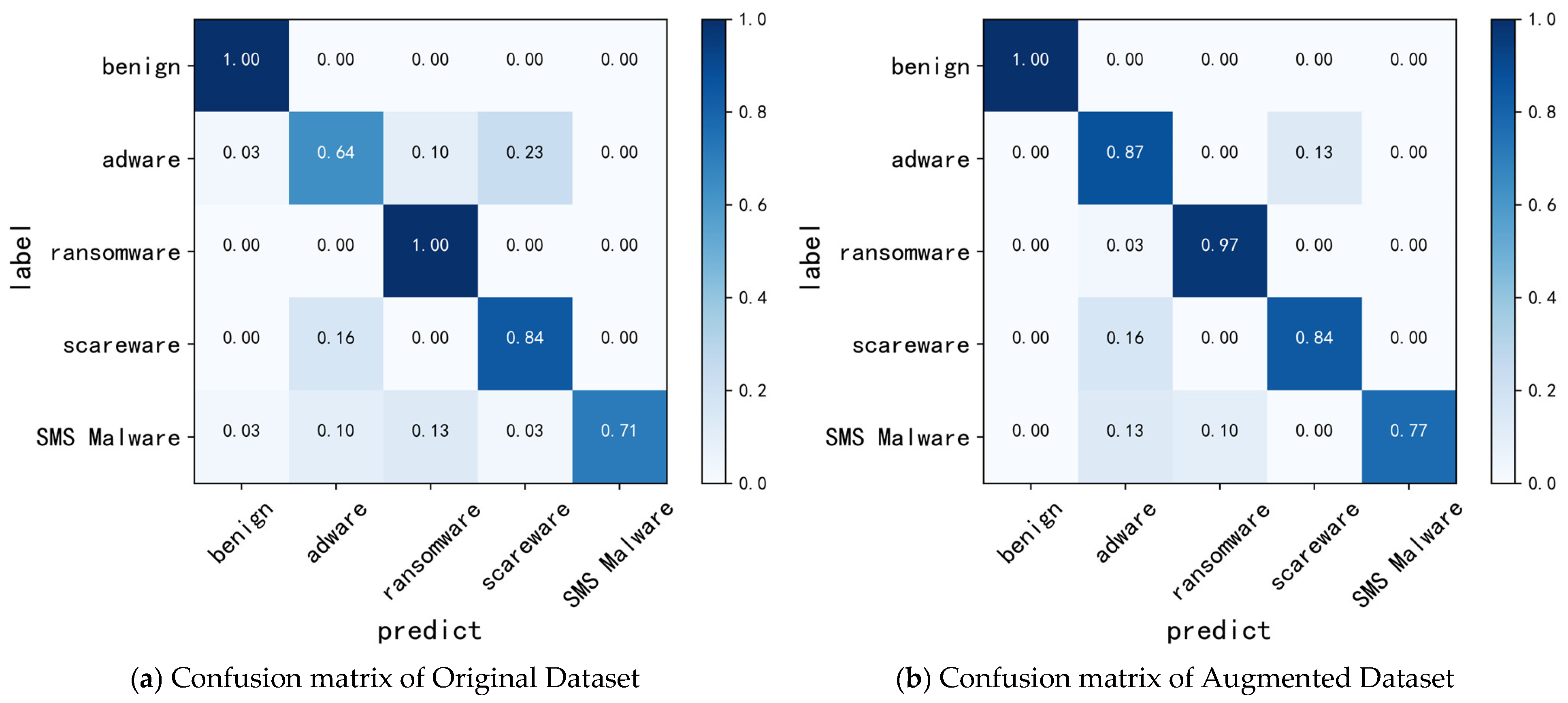
Figure 12 and Figure 13 display the confusion matrices of classification results before and after dataset augmentation, as well as for different models, providing an intuitive comparison of performance differences among the models. In these figures, the vertical axis represents the true classes, while the horizontal axis represents the predicted classes. A darker color along the diagonal indicates better classification performance. From Figure 12 and Figure 13, it is evident that compared to the original data, the performance of both the ResNet and SE-ResNet classification networks demonstrates a significant improvement after data augmentation using the WGAN.

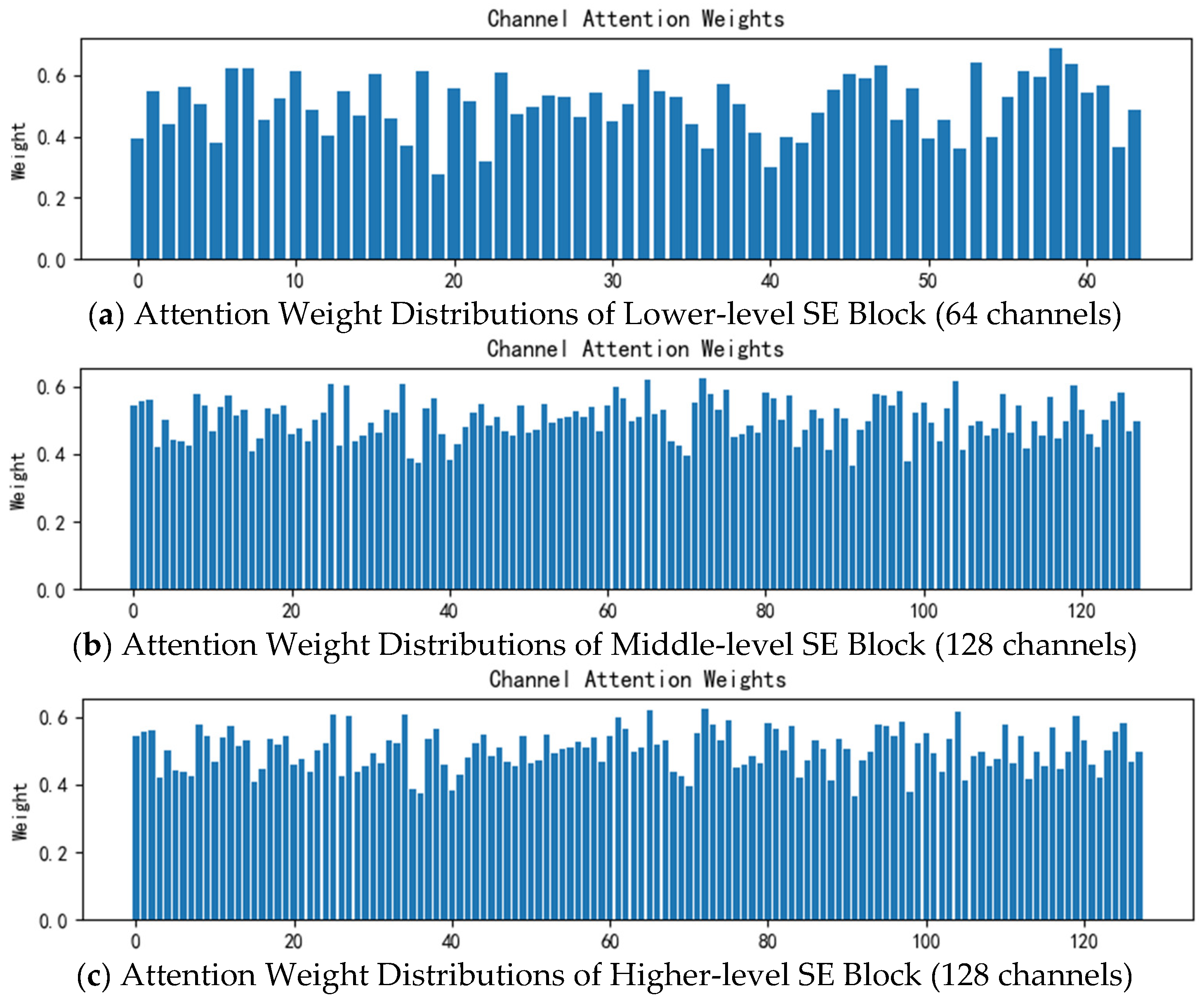
To investigate the operational mechanisms of the Squeeze-and-Excitation (SE) attention modules across different feature hierarchies, we visualized the channel attention weight distributions at three distinct network levels: lower, middle, and higher layers (as shown in Figure 14). Figure 14a displays the attention weights of the lower-level SE block (64 channels), where the distribution remains relatively uniform, indicating that the model broadly gathers information during the foundational feature extraction phase. Figure 14b presents the weights from the middle-level layer (128 channels), revealing a notable divergence in distribution. This suggests the model begins learning to discriminate between more and less important feature channels. Figure 14c illustrates the weights from the higher-level layer (256 channels), demonstrating a highly selective distribution. Here, the model concentrates its attention on a very limited number of critical channels, which are deemed essential for the final malware classification decision. This progressive evolution of attention focus, from shallow to deep layers, clearly demonstrates how our SE-ResNet model autonomously refines and extracts crucial discriminative patterns from the vast array of input features.

To validate the superior performance of the SE-ResNet model, a comparative experiment was designed, evaluating it against three baseline models—VGG, MobileNet, and SVM—on the same dataset. Among these, VGG and MobileNet are classical deep learning models, while SVM is a traditional machine learning model that requires converting grayscale images into feature vectors first. Simulation results are shown in

Table 12. Performances Comparison of Classification Models.

Classification Model	Precision	Recall	F1-Score
SE-ResNet	0.907	0.837	0.853
VGG	0.851	0.782	0.810
MobileNet	0.817	0.800	0.805
SVM	0.707	0.650	0.674

, from which we can note that the experimental results demonstrate that SE-ResNet exhibits superior performance across precision, recall, and F1-score. Although the VGG model achieved the highest precision (0.851), its recall was significantly lower (0.782), indicating limitations in its generalization capability. MobileNet, as a lightweight model, showed balanced but slightly reduced metrics (F1 = 0.805). In contrast, the traditional SVM method lagged significantly across all performance indicators (F1 = 0.674), highlighting the substantial advantage of deep learning models in feature learning. These findings confirm the advanced capabilities of the SE-ResNet model in image classification tasks.

4.3.3. Cross-Domain Experimentation

Railway malware samples do not typically disguise themselves as ordinary applications; instead, they highly imitate specific software such as ticketing apps, timetable query tools, or device maintenance programs. Their application names, icons, and interfaces are extremely similar to those of genuine software. Taking the “Railway 12306” client as an example, after its release, numerous counterfeit ticketing applications like “12306 Ticket Guru” and “12306 Train Tickets” appeared in Android app markets. The primary goal of such counterfeit apps is to steal private information or conduct ad fraud. For instance, in terms of network communication, the official 12306 app primarily communicates with official domains (e.g., *.12306.cn) and related CDN or cloud service providers using encrypted channels. In contrast, counterfeit apps often connect to unfamiliar IPs/domains and may transmit data in plaintext.

The process for establishing the railway sample set is as follows: (1) Collect APKs from mobile terminals (Android OS) used by various railway bureaus, and compute cryptographic hash algorithms (e.g., SHA-256, SHA-3) on the APKs to generate unique hash fingerprints; (2) Compare the APK hashes with mainstream malicious sample databases domestically and internationally to identify known threats. If a type of malware is not covered by mainstream databases but is explicitly defined as illegal software in railway industry regulations, it is also included in the malicious sample set for this experiment (e.g., counterfeit 12306 ticketing apps); (3) Aggregate known threat samples, remove duplicates, and compile the railway mobile terminal malware sample set. The current collection consists of 150 benign samples and approximately 100 deduplicated malicious samples from railway mobile terminals. These include 36 adware, 18 ransomware, 22 scareware, and 24 SMS Trojan malware samples, along with 150 benign samples.

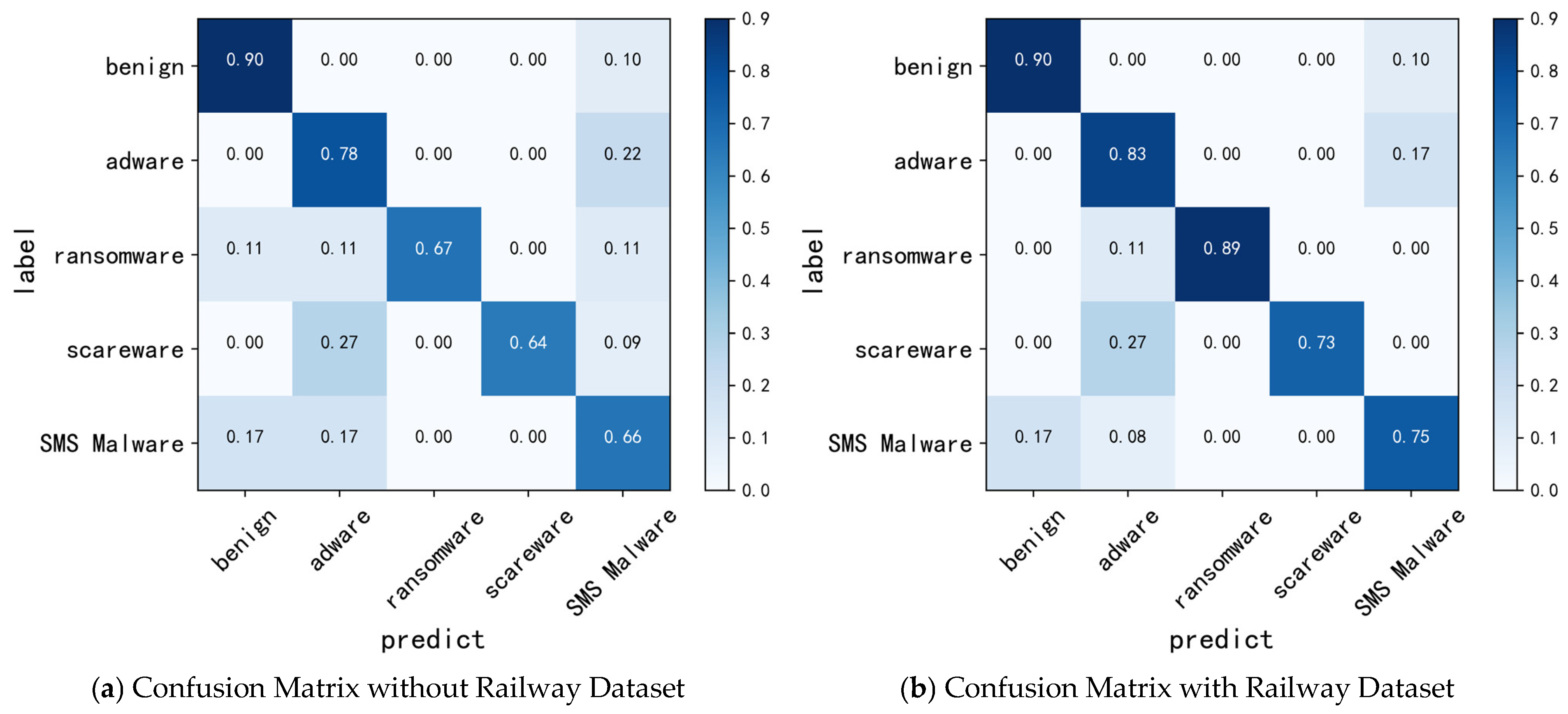
The datasets utilized in Section 4.3.1 and Section 4.3.2 were entirely sourced from the public dataset CIC-InvesAndMal2019. To accurately evaluate the classification model’s performance within the railway operational context, we isolated all railway-related benign and malware samples from the complete test set to construct a cross-domain railway scenario. Due to the scarcity of malware samples in the railway dataset, which makes it unsuitable for standalone WGAN-based data augmentation, this study integrated 50% of the railway dataset samples with the public dataset and performed unified augmentation using the WGAN framework. The combined dataset served as the training and validation sets for the cross-domain experiment, while the remaining 50% of the railway samples were reserved exclusively as the test set. The optimal model identified previously—the SE-ResNet classification model trained on augmented data—was subsequently evaluated on this test configuration.

Table 13. Sample Number Setting in Cross-domain Experiment.

Malware Families	Sample Number of Original Dataset	Sample Number with Railway Malware	Sample Number After Augmentation (Training-Validation Sample)	Test Sample Number with Railway Malware Percentage of 50%
adware	103	121	700	18
ransomware	97	106	700	9
scareware	105	116	700	11
SAM malware	105	117	700	12
benign	614	690	690	75

details the splits for the training, validation, and test sets used in the cross-domain experiment. The training-validation sets were constructed using 5-fold cross-validation (K = 5), where the counts represent the sample sizes after incorporating 50% of the railway samples and subsequent WGAN-based data augmentation.

Table 14. Performance Metrics of SE-ResNet Classification Model.

Type	Training Dataset Without Railway Sample			Training Dataset with Railway Sample
	Precision	Recall	F1-Score	Precision	Recall	F1-Score
benign	0.967	0.900	0.933	0.978	0.900	0.937
adware	0.700	0.777	0.737	0.75	0.833	0.789
ransomware	1.000	0.666	0.800	1.000	0.889	0.941
scareware	1.000	0.636	0.778	1.000	0.727	0.842
SMS Malware	0.333	0.676	0.447	0.409	0.75	0.529
average	0.800	0.729	0.763	0.828	0.819	0.824

presents the performance metrics of the SE-ResNet classification model before and after incorporating the railway dataset.

As can be seen from Table 14, after incorporating railway samples into the dataset, the newly trained model achieved an F1-score of 0.824 on the railway test samples, which is indeed slightly higher than the F1-score of 0.763 from the model trained without railway samples (an improvement of approximately 7.4%). This improvement is primarily attributable to the enhanced Recall rate (increased from 0.729 to 0.819), indicating a reduction in the missed detection rate of railway malware samples by the model. These metrics demonstrate that the model possesses the necessary conditions for migration to the railway mobile terminal malware detection scenario. Figure 15 displays the confusion matrices of classification results before and after dataset augmentation and for different models, further validating the results presented in Table 14.

4.4. Detailed Performance Analysis

To better illustrate the malware classification performance of the proposed model, this study further simulates four experimental configurations involving different classification models applied to the dataset both before and after augmentation. The simulations visually demonstrate the changes in the model’s loss curve, accuracy curve, P-R AUC curve, and ROC AUC curve as the number of iterations increases. Among these, the P-R AUC curve measures the trade-off between the model’s Precision and Recall on positive instances. It is highly sensitive to class imbalance and serves as a realistic indicator for evaluating the model’s performance in practical applications. The ROC AUC curve measures the model’s ranking ability, i.e., the probability that the model ranks positive instances higher than negative instances, and is insensitive to class imbalance. The specific results are shown in Figure 15, Figure 16, Figure 17 and Figure 18.

4.4.1. ResNet Model

(1)

Original Dataset

Figure 16 illustrates the performance of the ResNet classification model on the original dataset:

(a)

Loss Curve Analysis

As shown in Figure 16a, during the initial training phase, the training loss decreased rapidly from a high value of 1.4, indicating that the ResNet model quickly learned features from the data. As the number of training epochs increased, the training loss gradually plateaued and eventually stabilized at a relatively low value of 0.2, suggesting that the ResNet model was converging. The validation loss followed a similar trend but decreased at a slower rate, finally stabilizing around 0.3.

(b)

Accuracy Curve Analysis

As shown in Figure 16b, the training accuracy increased rapidly from a low initial value of 20% during the early stages of training, demonstrating the model’s capability to improve its classification performance quickly. With continued training, the training accuracy gradually stabilized, approaching nearly 100%, which indicates excellent classification performance on the training set. The validation accuracy followed a similar upward trend but at a slower pace, eventually stabilizing around 85%, slightly lower than the training accuracy. Analysis of the loss and accuracy curves reveals that although a certain gap exists between the training loss and validation loss, both metrics eventually stabilized, indicating that the model had converged. This suggests that the ResNet classification model possesses a certain degree of generalization capability and is capable of classifying malware. However, the relatively lower validation accuracy indicates a need for measures to improve accuracy further.

(c)

P-R AUC Curve Analysis

As shown in Figure 16c, the Micro-average AUC is 0.94, indicating reasonably good overall model performance. However, this favorable average is largely boosted by the perfect performance on the ‘benign’ class, which has the largest number of samples. In contrast, the P-R scores for ‘ransomware’ (0.64) and ‘scareware’ (0.53) are significantly lower, suggesting that the model produces a substantial number of false positives or false negatives for these classes. The P-R AUC curves indicate a severe performance imbalance during practical decision-making by the model, with poorer performance for classes having fewer samples.

(d)

ROC AUC Curve Analysis

As shown in Figure 16d, the Micro-average AUC is 0.98, indicating excellent performance in distinguishing positive and negative instances. The Macro-average AUC is 0.97, suggesting that all classes are well differentiated without any obvious weaknesses. The ROC AUC curves demonstrate that, from the perspective of distinguishing between positive and negative samples, this is a well-performing model.

(2)

Augmented Dataset

Figure 17 presents the training dynamics and final performance of the ResNet classification model on the WGAN-augmented dataset. The primary objective of this figure is to validate the fundamental improvement brought by the data augmentation strategy itself to the baseline model’s performance, thereby establishing a foundation for subsequent comparison with the advanced effects of SE-ResNet.

(a)

Loss Curve Analysis

As shown in Figure 17a, both the training and validation losses decrease smoothly and stabilize at low levels (training loss ≈ 0.2, validation loss ≈ 0.1). Crucially, the convergence trajectories of the two curves are closely aligned with a minimal gap. This directly demonstrates that data augmentation effectively expands the diversity of the training data, enabling the ResNet model to avoid overfitting and achieve superior generalization capability.

(b)

Accuracy Curve Analysis

Figure 17b shows that the model ultimately reaches and stabilizes at high levels on both the training and validation sets (training accuracy ≈ 100%, validation accuracy ≈ 95%). Compared to the baseline experiment using the original dataset, the validation accuracy is significantly improved, and no substantial gap appears between the training and validation curves. This indicates that the feature patterns learned by the model after data augmentation are more universal, rather than being a mere mechanical memorization of the training set.

(c)

P-R Curve and AUC Analysis

As evidenced by Figure 17c and

Table 15. Comparison of P-R-AUC.

Type	P-R-AUC Without Augmentation	P-R-AUC with Augmentation	Changes	Analyses
ransomware	0.643	0.964	↑ 0.321	The Most Improvement
scareware	0.532	0.844	↑ 0.312	Considerable Improvement
SMS Malware	0.850	0.941	↑ 0.091	Optimizing
adware	0.791	0.791	-	-
benign	1.000	1.000	-	-

, the model achieves a high Micro-average P-R AUC of 0.98. More importantly, the P-R AUC for all categories (including the malware families with fewer samples in the original data) reaches relatively high levels, demonstrating balanced performance distribution. This result clearly indicates that the WGAN data augmentation strategy successfully mitigates the class imbalance issue in the dataset. Consequently, the model maintains high Recall and Precision rates when confronting various threats, significantly enhancing its decision-making reliability in real-world scenarios.

(d)

ROC-AUC Curve Analysis

As shown in Figure 17d, the Micro-average AUC reaches 0.99, indicating the model possesses excellent overall discriminative ability between positive and negative samples. The Macro-average AUC of 0.99 demonstrates that the model performs exceptionally well in distinguishing each individual class, with balanced performance across all categories and no significant weaknesses. The ROC-AUC curves collectively confirm that this is a high-performing model from the perspective of binary classification capability.

4.4.2. SE-ResNet Model

(1)

Original Dataset

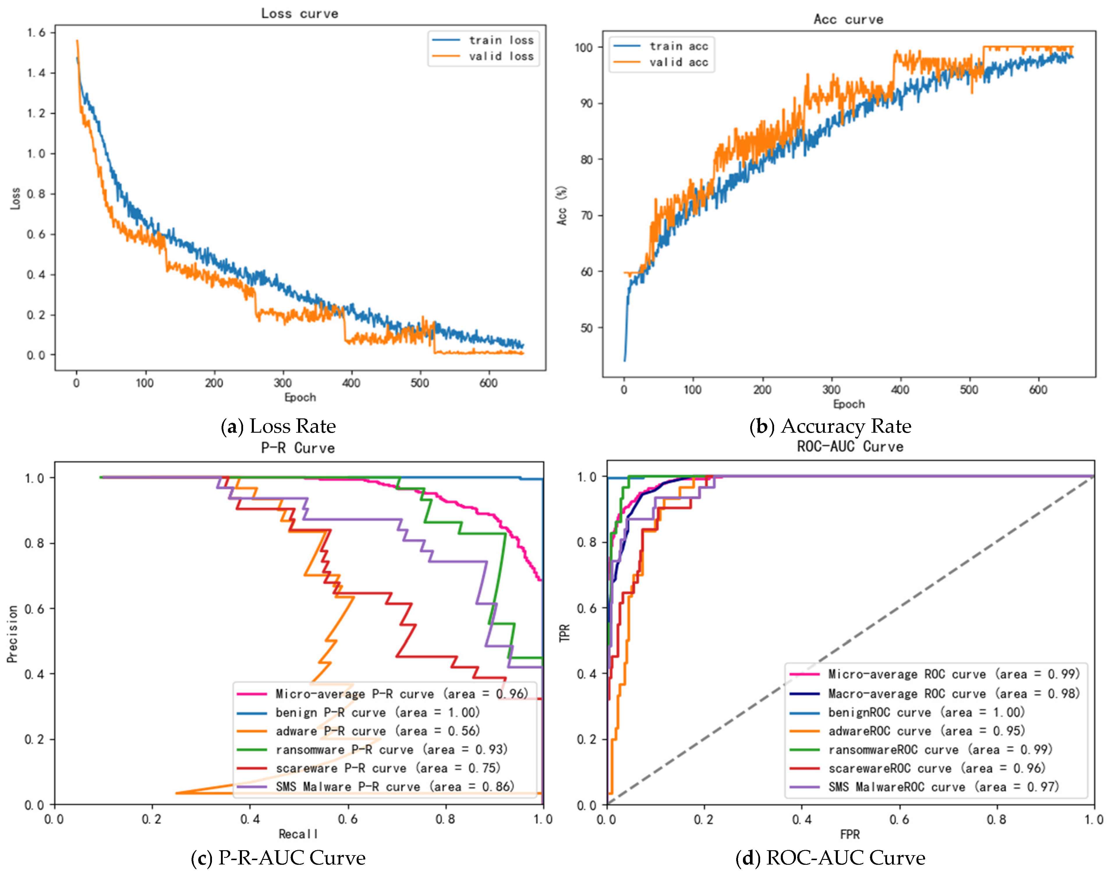
Figure 18 presents the training process and performance of the SE-ResNet classification model on the original dataset. The primary objective of this figure is to reveal the unique impact of the Squeeze-and-Excitation (SE) attention mechanism on model behavior and performance under baseline data conditions, thereby establishing a benchmark for subsequent comparison with data-augmented results.

(a)

Loss Curve Analysis

As shown in Figure 18a, the model loss eventually converges to a low level, indicating effective training. Compared to the ResNet model in Figure 16, the training loss curve of SE-ResNet exhibits greater volatility. This is not a training defect but rather a manifestation of the dynamic feature recalibration performed by its built-in SE modules. This mechanism enables the model to adaptively adjust channel weights for different samples, thereby enhancing its feature learning capability. However, this inherent dynamism introduces normal fluctuations in the loss curve.

(b)

Accuracy Curve Analysis

Figure 18b shows that the validation accuracy stabilizes at approximately 95% after convergence, representing an improvement over the baseline ResNet model. This result confirms the value of the SE modules: by emphasizing informative features and suppressing less useful ones, they enable the model to perform more efficient feature extraction, thus achieving a performance gain without additional data.

(c)

P-R Curve and AUC Analysis

As seen in Figure 18c, the model achieves a Micro-average P-R AUC of 0.96, superior to the ResNet’s 0.94. However, the P-R AUC for the Adware class is significantly lower (0.56), constituting the model’s primary weakness. This phenomenon clearly indicates that under the condition of original data imbalance, while the SE attention mechanism can improve overall performance, it struggles to fundamentally address the under-representation of minority classes (like Adware), resulting in suboptimal Recall and Precision for that specific category.

(d)

ROC Curve and AUC Analysis

Figure 18d shows that the model achieves high Micro-average and Macro-average ROC-AUC scores of 0.99 and 0.98, respectively, demonstrating its excellent overall classification performance. Nevertheless, the relatively lower AUC value for the Adware class further confirms the finding in Figure 18c: the model exhibits a degree of confusion when handling Adware samples, potentially misclassifying them as other categories (such as benign software or other malware types). This highlights the limitations of relying solely on architectural improvements and underscores the necessity of incorporating data augmentation to enhance the model’s classification performance.

(2)

Augmented Dataset

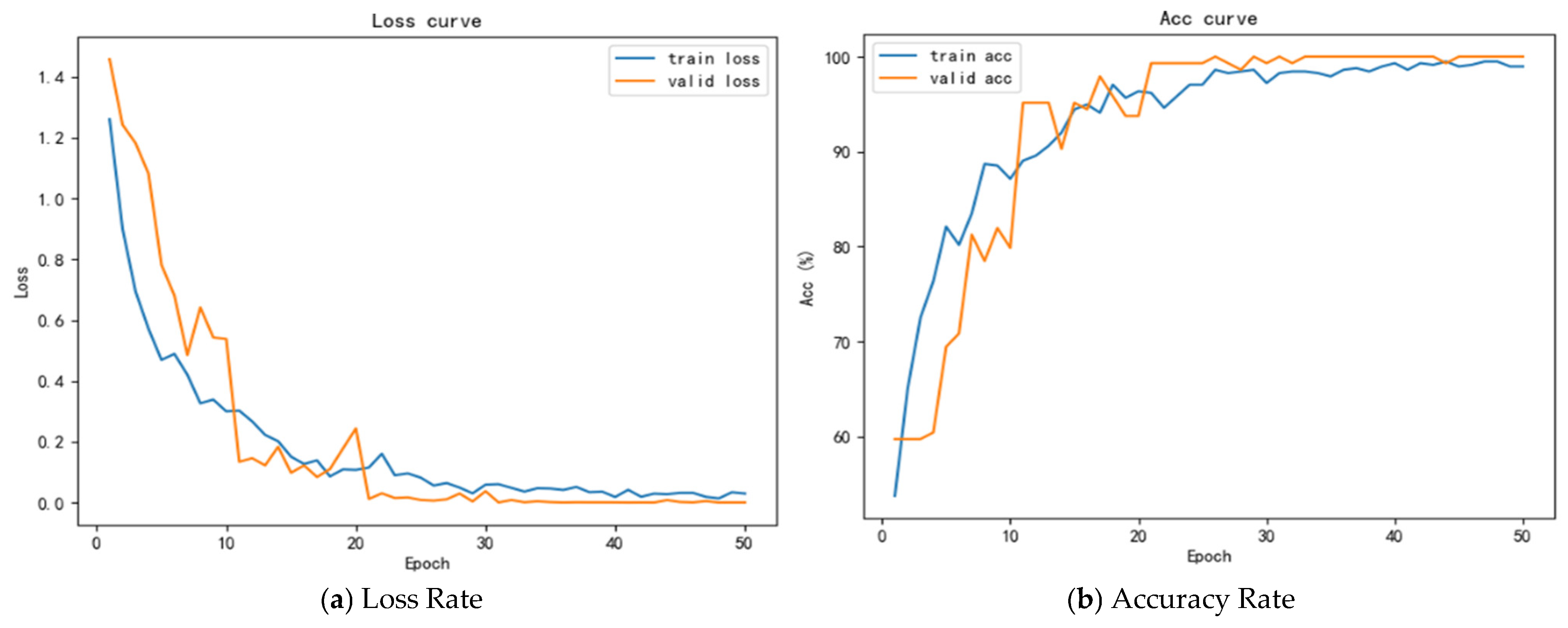
Figure 19 comprehensively presents the training dynamics and final performance of the SE-ResNet classification model on the WGAN-augmented dataset. The primary value of this figure lies in validating the combined effect of the data augmentation strategy and the SE attention mechanism: it ensures stable convergence during model training while significantly enhancing generalization performance and balance across all categories, particularly the minority classes.

(a)

Loss Curve Analysis

As shown in Figure 19a, the loss decreases rapidly during the initial training phase, indicating the model’s ability to quickly capture data features. As training progresses, both training and validation losses converge synchronously to low levels, with a minimal gap between them. This smooth and tightly aligned convergence trajectory demonstrates that data augmentation effectively expands the diversity of training samples, significantly mitigates overfitting, and endows the model with robust generalization capability on unseen data.

(b)

Accuracy Curve Analysis

Figure 19b shows that both training and validation accuracy rise rapidly and eventually stabilize at high levels, with validation accuracy reaching approximately 95%. A critical observation is the consistently narrow gap between the two curves and the absence of significant fluctuations. This further indicates that, after data augmentation, the model no longer merely memorizes the training set but instead learns more universal classification features, resulting in consistent performance on both training and validation data.

(c)

P-R Curve and AUC Analysis

As evidenced by Figure 19c and

Table 16. Comparison of P-R-AUC.

Type	R-AUC Without Augmentation	R-AUC with Augmentation	Changes	Analyses
ransomware	0.930	0.981	↑ 0.051	Slight Improvement
scareware	0.750	0.892	↑ 0.142	Significant Improvement
SMS Malware	0.864	0.974	↑ 0.130	Significant Improvement
adware	0.562	0.863	↑ 0.301	Considerable Improvement
benign	1.000	1.00	-	-

↑ means increasing.

, the model achieves a Micro-average P-R AUC of 0.98, with excellent P-R AUC performance across all categories. This result is particularly significant, as it indicates that the data augmentation strategy substantially benefits malware categories with smaller sample sizes, preventing the model from developing discriminatory bias due to the original imbalance in data distribution. Compared to the ResNet results in Figure 17, the improved balance in SE-ResNet validates the effectiveness of the attention mechanism in capturing critical patterns within complex feature environments.

(d)

ROC Curve and AUC Analysis

Figure 19d demonstrates that the ROC-AUC values for all categories approach 1.00. The high Macro-average AUC of 0.99 indicates that the model achieves excellent classification performance for each individual category, regardless of sample size. This validates the core proposition of this study—that combining WGAN data augmentation with the SE-ResNet classification model can construct a high-performing malware detection system capable of effectively meeting operational requirements for high Recall rates across all threat categories in practical deployment scenarios.

Based on the comprehensive experimental analysis presented above, the algorithm that employs WGAN for data augmentation and SE-ResNet for classification, as illustrated in Figure 19, demonstrates superior performance over the ResNet model across three critical metrics—precision, recall, and F1-score—when evaluated on the same input dataset. The analyses of the loss curves, accuracy curves, P-R AUC curves, and ROC AUC curves in Section 4.4 further corroborate the results presented in Section 4.3.

In high-stakes operational environments like railway systems, the cost of a false negative (failing to detect malware) far exceeds that of a false positive (misclassifying benign software). A single missed detection could lead to security incidents and service disruptions, resulting in significant economic and reputational damage. In contrast, false alarms can typically be resolved through manual review, representing a relatively manageable cost. Therefore, achieving a high Recall rate is generally the prioritized performance objective for classification models in practical railway deployment. Railway operators can dynamically adjust the classification decision threshold based on current security policies and the acceptable cost of false positives. For instance, during periods of elevated security threat levels, the decision threshold for the malware class could be lowered to pursue higher Recall rates. Conversely, during routine operations, the threshold could be appropriately raised to balance the operational burden caused by false alarms. The performance demonstrated by the SE-ResNet model, selected through multiple ablation experiments in this work, shows consistently strong results specifically in the Recall metric. This provides a reliable baseline operational point for railway deployment scenarios.

5. Conclusions

This paper proposes a malware detection model for railway mobile terminals based on a WGAN and an SE-ResNet architecture. Firstly, by executing malware samples from the publicly available CIC-InvesAndMal2019 dataset and those collected from railway mobile terminals in a real-world environment, typical processes were selected, memory features were captured, and these malware characteristics were converted into grayscale images, thereby establishing the original dataset. Secondly, a WGAN was employed for data augmentation to mitigate sample insufficiency and class imbalance, as well as to reduce overfitting in the classification model. Thirdly, a ResNet34-based network model was utilized to extract features from the grayscale image samples, with important features being weighted. Through multi-level feature convolution, optimal training results were obtained. By integrating an attention mechanism module into the residual units, an SE-ResNet model was constructed, enabling the classification model to more accurately extract key features from the grayscale images. Multiple sets of experiments demonstrated that the optimized model significantly enhances generalization capability and improves malware detection performance. Finally, through multiple training iterations, a malware detection model for railway mobile terminals was obtained. The detection model proposed in this paper can serve as a reference and provide insights for the future development of malware detection tools for mobile terminals in the railway industry.

References

- TJ/XX 013-2024; Guidelines for Railway Cybersecurity Inspection (Provisional). China State Railway Group Co. Ltd.: Beijing, China, 2024.
- Meng, L.; Wanping, L.; Dong, H. Malicious Code Detection Based on Feature Fusion. Comput. Eng. Des. 2024, 45, 3568–3574. [Google Scholar]
- Zhi, Z.; Yukai, Y.; Yiling, S.; Wenjin, M.; Chang, P. Research on Android Malware Detection Model Based on Multimodal Feature Fusion. Comput. Eng. 2025, 1–12. Available online: https://aipub.cn/JzH87N5 (accessed on 19 August 2025).
- Benhui, F.; Jiayang, W. A Malicious Code Detection Technology Based on Static API Calls and Ensemble Learning. Sci. Technol. Inf. 2013, 9, 32. [Google Scholar]
- Chijun, L. Research and Implementation of Malicious Code Detection System Based on Heuristic Algorithm [D]. Ph.D. Thesis, Nanjing University of Posts and Telecommunications, Nanjing, China, 25 January 2025. [Google Scholar]
- Zhiwen, W.; Guangqi, L. A Survey of Malware Recognition Research Based on Machine Learning. J. Chin. Comput. Syst. 2022, 43, 2628–2637. [Google Scholar]
- Ying, T.; Bowei, N.; Yu, Z.; Qi, Z. Malicious Code Behavior Detection Method Based on Sandbox Technology. J. Xi’an Univ. Posts Telecommun. 2018, 23, 101–110. [Google Scholar]
- Weiping, W.; Shichen, Z.; Han, W.; Lin, S. A Linux Malware Detection Scheme Based on Virtual Machine Introspection. Netinfo Secur. 2024, 24, 657–666. [Google Scholar]
- Xiaolong, C.; Chuanjie, J.; Xin, L.; Min, Z. Design and Implementation of a Lightweight Linux Sandbox Based on Multiple Security Mechanisms. Res. Explor. Lab. 2023, 42, 83–87. [Google Scholar]
- He, K.; Zhang, X.; Ren, S.; Sun, J. Deep residual learning for image recognition. In Proceedings of the IEEE Conference on Computer Vision and Pattern Recognition, IEEE Computer Society, Las Vegas, NV, USA, 27–30 June 2016; pp. 770–778. [Google Scholar]
- Ziheng, R. Research and Implementation of Malicious Code Detection Technology Based on Deep Learning. Ph.D. Thesis, Beijing University of Posts and Telecommunications [D], Bejing, China, 2024. [Google Scholar]
- Shuhui, Z.; Changdong, H.; Lianhai, W.; Shujiang, X.; Wei, S.; Tian, L. Malicious Code Detection and Classification Based on GHM Visualization and Deep Learning. J. Inf. Secur. Res. 2024, 10, 216–224. [Google Scholar]
- Yin, J.; Ning, C.; Tang, T. Data-driven models for train control dynamics in high-speed railways: LAG-LSTM for train trajectory prediction. Inf. Sci. 2022, 600, 377–400. [Google Scholar]
- Chaoyuan, S.; Qiuhua, J.; Dongping, X.; Qi, L. A Ransomware Classification Method Based on Hilbert Curve-Residual Network. Comput. Technol. Dev. 2023, 33, 153–159. [Google Scholar]
- Li, L. A Cybersecurity Situation Awareness Method Based on Residual Convolutional Neural Network. Mod. Comput. 2024, 30, 56–60. [Google Scholar]
- Bo, X.; Guowei, S.; Chun, G.; Yan, Z.; Miao, Y. A Cybersecurity Entity Recognition Method Based on Residual Dilated Convolutional Neural Network. J. Cyber Secur. 2020, 6, 13–21. [Google Scholar]
- Yang, Z.; Jiangbo, H. Malicious code detection method based on attention mechanism and residual network. J. Comput. Appl. 2022, 42, 1708–1715. [Google Scholar]
- Goodfellow, I.J.; Pouget-Abadie, J.; Mirza, M.; Xu, B.; Warde-Farley, D.; Ozair, S.; Courville, A.; Bengio, Y. Generative adversarial networks. In Proceedings of the International Conference on Neural Information Processing System, Montreal, QC, Canada, 8–13 December 2014; MIT Press: Cambridge, MA, USA, 2014. [Google Scholar]
- Ledig, C.; Theis, L.; Huszár, F.; Caballero, J.; Cunningham, A.; Acosta, A.; Aitken, A.; Tejani, A.; Totz, J.; Wang, Z.; et al. Photo-realistic single image super-resolution using a generative adversarial network. In Proceedings of the IEEE Conference on Computer Vision and Pattern Recognition, Honolulu, HI, USA, 21–26 July 2017; pp. 4681–4690. [Google Scholar]
- Bai, Y.; Zhang, Y.; Ding, M.; Ghanem, B. Sod-mtgan: Small object detection via multi-task generative adversarial network. In Proceedings of the European Conference n Computer Vision (ECCV), Munich, Germany, 8–14 September 2018; pp. 210–226. [Google Scholar]
- Yu, L.; Zhang, W.; Wang, J.; Yong, Y. Seqgan: Sequence generative adversarial nets with policy gradient. In Proceedings of the AAAI Conference on Artificial Intelligence, San Fracisco, CA, USA, 4–9 February 2017. [Google Scholar]
- Arjovsky, M.; Chintala, S.; Bottou, L. Wasserstein generative adversarial networks. In Proceedings of the International Conference on Machine Learning, PMLR, Sydney, NSW, Australia, 6–11 August 2017; pp. 214–223. [Google Scholar]
- Arjovsky, M.; Bottou, L. Towards principled methods for training generative adversarial networks. arXiv 2017, arXiv:1701.04862. [Google Scholar] [CrossRef]
- Li, L.; Qing, Z.; Youran, K.; Renjia, S.; Xin, Z. A Family Tracing Method for Malicious Code Variants Based on Generative Adversarial Networks. Comput. Eng. Sci. 2025, 47, 1215–1225. [Google Scholar]
- Jiaxuan, W.; Xiaojuan, W.; Mingshu, H.; Xinlei, W.; Zikui, L. An Imbalanced Data Augmentation Method Based on Generative Adversarial Networks for Intrusion Detection. Inf. Secur. Commun. Priv. 2024, 12, 22–34. [Google Scholar]
- Burks, R.; Islam, K.A.; Li, J.; Lu, Y. Data Augmentation with Generative Models for Improved Malware Detection: A Comparative Study. In Proceedings of the IEEE 10th Annual Ubiquitous Computing, Electronics & Mobile Communication Conference, IEEE, New York, NY, USA, 10–12 October 2019. [Google Scholar]
Figure 1.
Overall Framework.
Figure 3.
SE-ResNet Network.
Figure 5.
WGAN Framework.
Figure 2.
ResNet34 Network Architecture Diagram.
Figure 6.
Simulation Process.
Figure 7.
Memory Feature Extraction Process.
Figure 8.
Grayscale Image from Selected Data.
Figure 9.
Loss Function of Generator and Discriminator.
Figure 10.
Real Image and Fake Image in the First Epoch.
Figure 11.
Real Image and Fake Image after Training.
Figure 12.
Confusion Matrix of the ResNet.
Figure 13.
Confusion Matrix of the SE-ResNet.
Figure 14.
Attention Weight Distributions.
Figure 15.
Confusion Matrix of SE-ResNet with or without Railway Dataset.
Figure 16.
ResNet Classification Performances under Original Dataset.
Figure 17.
ResNet Classification Performances under Augmented Dataset.
Figure 18.
SE-ResNet Classification Performances under Original Dataset.
Figure 19.
SE-ResNet Classification Performances under Augmented Dataset.