Abstract
In Liquid Composite Molding (LCM), the high variability present in reinforcement properties such as permeability creates additional challenges during the injection process, such as void formation. Although improved injection strategy designs can mitigate the formation of defects, these processes can benefit from real-time process monitoring and control to adapt the injection conditions when needed. In this study, a machine vision algorithm is proposed, with the objective of detecting and tracking both fluid flow and bubbles in an LCM setup. In this preliminary design, 3D-printed porous geometries are used to mimic the architecture of textile reinforcements. The results confirm the applicability of the proposed approach, as the detection and tracking of the objects of interest is possible, without the need to incur in elaborate experimental preparations, such as coloring the fluid to increase contrast, or complex lighting conditions. Additionally, the proposed approach allowed for the formulation of a new dimensionless number to characterize bubble transport efficiency, offering a quantitative metric for evaluating void transport dynamics. This research underscores the potential of data-driven approaches in addressing manufacturing challenges in LCM by reducing the overall process monitoring complexity, as well as using the acquired reliable data to develop robust, data-driven models that offer new understanding of process dynamics and contribute to improving manufacturing efficiency.
1. Introduction
Recent advances in machine learning, namely in convolutional neural networks, provided powerful means of image segmentation with the further advantage of achieving fast learning rates. This approach has given valuable results in a wide variety of fields, including composite material manufacturing, where machine learning solutions have been proposed in areas such as defect determination in laminates, through different destructive and non-destructive methods [1,2,3]. Overall, the proposed methodologies showed promise in aiding the task of laminate quality assessment after manufacturing, which can be automated to reduce the necessary time to conduct the tests and provide more reliable results than current image thresholding approaches.
Although inspection is a necessary step in the quality assurance of the manufactured parts, the information provided can only be gathered after both process design and part manufacturing are completed. In turn, following this methodology alone, trial-and-error experimental programs have to be employed in order to find improved process design iterations, which can have a significant impact on both design development time and cost [4].
Liquid Composite Molding (LCM) is a family of composite manufacturing processes, in which liquid resin is injected inside a closed mold, where a dry fibrous reinforcement is placed, in order to be permeated [4]. The flow of resin and subsequent reinforcement impregnation follow Darcy’s law, by which the volume-averaged flow velocity depends on the imposed pressure gradient, the fluid viscosity , and the permeability tensor of the porous medium , as stated in Equation (1).
In turn, the flow-front position during mold filling will depend on variables such as permeability, the stochastic nature of which may introduce high variability [5]. The inherent uncertainty in permeability arises from multiple ambiguously correlated factors, including reinforcement intrinsic defects, textile microstructure variations, and inconsistent manufacturing conditions [6]. Flow disturbances are further caused by race-tracking along the edges and corners of the mold, where small channels or gaps between the preform edge and cavity wall create areas of significantly increased permeability due to fabric placement imperfections [7,8]. Also, the transport of voids within the mold directly impacts the quality of the final part, with the literature demonstrating a significant reduction in mechanical properties, with only a marginal void content in fiber-reinforced composites [9]. This makes predictive understanding of void transport behavior essential for maximizing part performance and reducing manufacturing defects.
In a way, to circumvent the shortcomings of trial-and-error process design, several methodologies have been proposed, in which mold filling simulations are used, in combination with stochastic parameters [10]. Mathematical frameworks for stochastic RTM processes have been developed to understand how random permeability fields affect filling behavior [11]. As the end goal, the improved injection design should be robust towards any variability present in the system.
In parallel, research in LCM has also focused on the study of systems capable of conducting real-time monitoring and control of the mold-filling process to counteract these uncertain variabilities. Different approaches have been suggested, from using sensor arrays to monitor flow-front [12,13], to activating control strategies based on selective injection [14], or localized heating to adjust resin viscosity [15]. Recent advances in machine learning have demonstrated particular promise, with physics-informed neural networks enabling real-time prediction of resin flow behavior [16]. Generative adversarial networks have shown considerable potential for flow-front prediction with statistical validation across diverse manufacturing scenarios [17]. Moreover, due to the employed machine vision algorithms, some systems require additional experimental preparation, either by the use of a coloring agent mixed with the fluid or precise lighting conditions to increase the contrast between saturated and non-saturated regions of the reinforcement [18].
To overcome these shortcomings, this study proposes an algorithm based on a convolutional neural network architecture to detect and track the fluid flow, as well as bubbles generated throughout the flow process during the filling of the mold. Unlike existing machine vision approaches that require fluid-coloring agents or specialized lighting conditions [18], or sensor-based methods limited to point measurements [12,13,17], the proposed algorithm operates under standard experimental conditions while providing spatially distributed monitoring capabilities. As a testbed, a 3D-printed porous geometry resembling the meso-scale architecture of a reinforcement textile [19] is used in the flow experiments, thus allowing for the validation of the applicability of the algorithm. While this simplified geometry cannot capture the full complexity of real textile reinforcements—including dual-scale porosity, stochastic fiber placement variations, and deformable tow structures—this deliberate simplification serves a critical methodological purpose. The well-characterized, low-variability system enables the confident measurement of fundamental bubble transport mechanisms and rigorous validation of the machine learning algorithm against known ground truth, which would be impossible in highly variable real fabrics where algorithmic performance cannot be separated from material variability.
Based on experimental data processed by the algorithm, a new data-driven bubble transport model is proposed, enabling a fast estimation of bubble mobility. The current paper develops upon the previous work [20] by introducing the steps needed for building a real-time monitoring system. The current study also demonstrates the performance across different 3D printing technologies, providing insights into how surface characteristics affect bubble and flow-front detection accuracy—considerations essential for translating the methodology to diverse manufacturing environments. Lastly, this work introduces a novel dimensionless parameter that consolidates bubble transport efficiency into a single metric, enabling quantitative process optimization beyond the separate parameter analysis presented in [20].
2. Materials and Methods
2.1. Experiments
In this study, fluid flow experiments were conducted using a calibrated ideal porous medium architecture, already tested for permeability characterization, which loosely resembles the meso-scale architecture of a textile fabric used in composite reinforcements [19], with the dimensions depicted in Figure 1. The geometry was produced with additive manufacturing in which the geometrical structures resembling the fiber tows were converted to solid blocks.
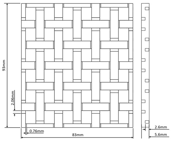
Figure 1.
Porous medium dimensions.
The smaller features of the gaps within the fiber tows were not possible to manufacture, but it is well known that as fiber tows are small and densely packed, assuming them to be solid tows may not be a far-fetched assumption in terms of tracking the flow and bubbles.
Two different specimens of the geometry were manufactured using two different 3D printing technologies: Multi-Jet Fusion (MJF) (HP, Palo Alto, CA, USA) and Stereolithography (SLA) (Formlabs, Somerville, MA, USA). Although these 3D printing processes provide different surface characteristics, as presented in Table 1 [21], which may affect the fluid flow, the main focus of this study relies on the visual aspect of the porous medium to accurately track the bubbles in the flowing fluid and quantify its impact on image segmentation quality. A depiction of the visual differences between the MJF- and SLA-printed porous media is shown in Figure 2.

Table 1.
Surface roughness of the manufactured parts.
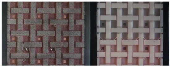
Figure 2.
Visual images of MJF (left) and SLA (right) 3D-printed porous media with test fluid and formed bubbles.
The mold cavity was created with a top and bottom plate with the ideal porous media manufactured by AM sandwiched in between and surrounded by a metallic frame. Motor oil (properties listed in Table 2) was used as simulated resin and injected into the mold. Motor oil is a good replacement for actual resin, since its rheologic properties are similar to the ones found in LCM resins and are more stable (do not suffer from curing effects). This provides more confidence in the results of this study, as the fluid properties do not change during the experiment. The top transparent PMMA plate allowed for the visual monitoring of the fluid flow-front and the bubbles inside the porous medium. This experimental setup was used to measure the permeability of the ideal AM porous structure, with an uncertainty in its characterization provided in [19].
Table 2.
Properties of motor oil, the test fluid.
Each experiment starts with the dry porous medium placed inside the mold cavity, and when the inlet is opened, the test fluid starts to flow through the open channels within the porous medium, which naturally generates bubbles by mechanical air entrapment, similarly to what can be observed in LCM manufacturing. An example of bubble formation through the flow-front mechanical air entrapment is depicted in Figure 3. In each experiment, a constant flowrate was imposed using an Isojet® pump system (Isojet, Corbas, France), ranging from 10 g/min to 100 g/min. The flow-front progression and bubble formation inside the porous medium were recorded by a video camera (Teledyne, Thousand Oaks, CA, USA), filming with a resolution of 1280 × 720 pixels at 50 frames per second. No fluid-coloring agents or other contrast-enhancing techniques to ease the segmentation task were used to validate the generic applicability of the proposed methodology, thus eliminating the need for elaborated LCM setups. It is important to emphasize that the decision to avoid fluid-coloring agents or enhanced lighting conditions was not merely for experimental simplicity but rather to validate the algorithm’s performance under realistic, close-to-industrial conditions, where such preparations may be impractical or undesirable. This approach ensures that the proposed methodology can be more readily implemented in actual LCM manufacturing environments without requiring specialized experimental setups.
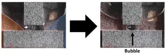
Figure 3.
Void formation due to air entrapment between merging flow-fronts: merging flow-fronts highlighted in orange and blue (left), leading to bubble formed by mechanical air entrapment (right).
2.2. Algorithm Overview
The developed algorithm conducts an analysis on a frame-by-frame basis, from the video recording, as shown by the flowchart in Figure 4. Until the end condition is met, the algorithm extracts a new frame from the video feed and segments it. This segmentation procedure allows for the subsequent detection of all objects of interest (bubbles and fluid flow-front), as well as the processing of their relevant properties, such as area, perimeter, and position in the selected frame. Finally, due to the high number of bubbles that can be generated in experiments, a tracking algorithm was formulated to ensure that the measured properties are assigned to the correct bubble, by which a unique label is attributed to each newly detected bubble in the video feed. Thus, the general algorithm can be divided into two main modules: video frame acquisition and segmentation, and bubble and flow-front tracking. All modules were developed using the Python (version 3.10) programming language. The detailed functioning of these modules is elaborated on in the following sections.
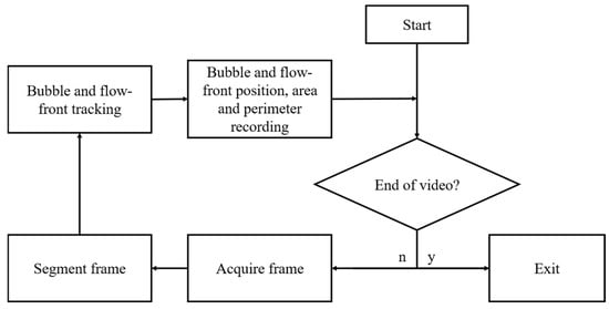
Figure 4.
Flow-front and bubble detection, characterization, and tracking algorithm flowchart.
2.3. Image Segmentation: Network Architecture
The implemented network architecture is similar to the original U-Net architecture [22], with a few modifications. The U-Net architecture was selected due to its proven effectiveness in segmentation tasks requiring precise boundary detection, particularly in biomedical applications where accurate object delineation is critical. While direct comparisons with similar applications in LCM flow-front and bubble monitoring were not found in the literature, the architectural modifications implemented here were tailored to address the unique challenges of bubble and flow-front detection in porous media flow.
The contracting path is constructed by stacking successive 3 × 3 convolution layers, each followed by a rectified linear unit (ReLU). The down-sampling of the feature map is accomplished by using 2 × 2 maximum pooling layers after each pair of convolution layers. The expansive path is composed of four similar blocks. Each block possesses a 2 × 2 transposed convolution layer, in which the resulting feature map is then concatenated to its corresponding pair of the contracting path. Finally, to the resulting concatenation follows a pair of 3 × 3 convolution layers and an ReLU activation.
Before each block, a dropout layer was added, as means of avoiding overfitting [23]. The dropout rate was adjusted to prevent overfitting given the dataset size while maintaining sufficient network capacity for accurate segmentation. A 1 × 1 convolution layer is added to the end of the network, to map the components of the feature vector to the desired number of classes, followed by soft-max activation, to map the output of the network to a probability distribution over the predicted classes. The four-class segmentation approach (flow-front, bubble core, bubble edge, and background) was specifically designed for this application, as explained in Section 2.4. The network model was implemented in TensorFlow using Keras [24].
2.4. Dataset
The dataset used in this study is composed of video frames extracted from the experimental recordings of fluid flow in the 3D-printed representative porous media. To test the influence of the visual differences between the porous media, frames were extracted from experiments with both types of porous media. Since the porous medium became increasingly saturated by the test fluid during the experiments, the capturing of the flow-front progression is a relevant aspect of the machine vision algorithm, and thus frames with different levels of flow-front progression were included in the dataset.
Three different types of datasets were created: the training dataset, the test dataset, and the validation dataset. The training dataset, which is used to update the parameters of the network, is composed of 300 sub-frames of MJF experiments and 150 sub-frames of SLA experiments, with a resolution of 512 × 512 pixels. In parallel, a test dataset was used to assess the performance of the network during each training epoch, thus allowing for the detection of over- or underfitting. The test dataset is composed of 100 sub-frames of MJF experiments and 50 sub-frames of SLA experiments, also with a resolution of 512 × 512 pixels. All sub-frames were extracted randomly from original video frames, which were selected from different experiments in a random fashion. To evaluate the performance of the network after training, a validation dataset was created, which possesses ten complete video frames from MJF and SLA-printed porous media flow experiments (twenty frames for validation, in total) with a resolution of 1280 × 720 pixels. Again, all video frames were extracted randomly from different experiment video recordings.
To create the ground-truth masks, an image with resolution equal to the original frame is created, where the output classes are one-hot-encoded in RGB format. In this study, four different classes are intended: flow-front (encoded in green channel), bubble core (encoded in red channel), bubble edge (encoded in blue channel), and background (encoded in black—all channels have null pixel intensity). The flow-front class refers to the area occupied by the fluid, whereas the bubble core class encompasses the central region of the bubbles, up to the border region. The bubble edge class refers to the border region of the bubbles, the width of which is about 1 pixel. The idea behind the implementation of this class is to avoid the implementation of post-processing algorithms such as watershed separation, which would be necessary to define the contour of touching bubbles, if only the bubble core class was implemented. In turn, a more reliable segmentation is expected using this strategy since actual morphological data are used, as well as faster post-processing times since there is no need to implement additional algorithms. The background class refers to the regions which do not provide any object of interest. A depiction of all classes is provided in Figure 5.
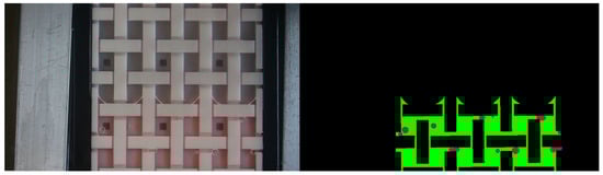
Figure 5.
Segmentation classes—red: bubble core; blue: bubble edge; green: flow-front; black: background.
2.5. Training
During the training procedure, the images were fed to the network in batches. This strategy allows for training to be conducted without incurring GPU memory overloads, while keeping ten images per batch, favoring the training convergence. The Adam optimization algorithm [25] was used with an initial learning rate of 0.001, and the number of batches per epoch was calculated so that all 512 × 512 images would theoretically be processed during an epoch. The selection of the images per batch was randomized. A total of 100 training epochs were conducted. Due to the highly unbalanced segmentation classes present in the dataset, boundary loss [26] was favored over weighted categorical cross-entropy or dice loss, as it provided improved results, especially in the bubble edge regions, which correspond to the least dominant class.
From the plots in Figure 6, which register the loss computed in the training and test datasets, during the training procedure, it can be observed that no evident signs of overfitting exist. After sixty training epochs, no noticeable improvements exist. However, possibly due to the different appearance of the porous media, as well as other features present in each dataset, the learning curves differ slightly. Occasional spikes in the loss function (visible around epochs 25 and 60) are attributed to the stochastic nature of randomized batch selection and the unbalanced class distribution but do not indicate training instability, as evidenced by the consistent convergence behavior and final model performance. The final U-Net models were trained using both the training and test datasets.
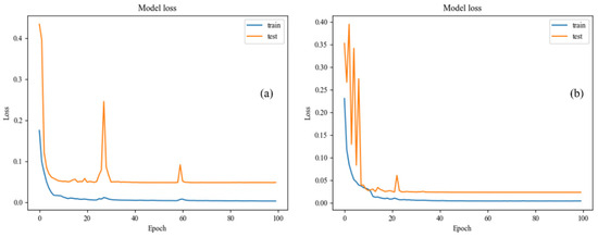
Figure 6.
Registered training and validation losses for (a) MJF dataset; (b) SLA dataset.
2.6. Bubble and Flow-Front Tracking
The tracking algorithm is responsible for tracking the bubble centroid position in the image, as well as the bubble area and perimeter at each processed frame. Bubble area, perimeter, and centroid position data are obtained using the contours of each bubble obtained from the bubble core class, using well-established methods provided in the OpenCV library [27].
To correlate bubbles from former to subsequent video frames, an object tracker algorithm was used. Correlation filter tracking algorithms are part of the current state of the art in object tracking [28]. The MOSSE algorithm [29] is capable of tracking object translations, as well as rotation and occlusion, at a frame rate of 669 frames per second. The fDSST algorithm [30] builds on the MOSSE algorithm to account for variations in the scale of the objects of interest. This increases tracking reliability; however, the added complexity reduces the computational speed to 24 frames per second [30]. In this study, to accommodate for volume changes in bubbles, due to pressure variations, as well as bubble splitting or coalescence, the fDSST algorithm was preferred over the MOSSE algorithm, and an implementation available in the Dlib library was used [31]. To further increase the reliability of the tracking procedure, a set of additional heuristics were implemented, on top of the object tracking algorithm. The bounding boxes of the segmented bubble contours are compared to the bounding boxes predicted by the tracking algorithm. The tracking algorithm bounding boxes that match the contour bounding boxes (given a set of dimensional and positional tolerances) are assumed to belong to the same bubble. Otherwise, the tracking algorithm bounding boxes that are left unmatched are discarded, and the contour bounding boxes that are unmatched are regarded as new bubbles. In turn, two hyperparameters are needed for the implementation of the additional heuristics: maximum radius of search and maximum admissible bubble area change between frames. A unique identifier is given to each newly detected bubble, as means of keeping a consistent property record throughout the video capture. Regarding flow-front tracking, since there is a single flow-front in the video recording, the position of the flow-front is computed using its most extreme point from the extracted contour. A representation of the tracking process is depicted in Figure 7, where two different video frames were extracted 1.6 s apart, for comparison.
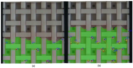
Figure 7.
Representation of the tracking procedure: (a) current time-step; (b) 1.6 s later time-step. Fluid highlighted in green, bubbles highlighted in red. Cross and dashed lines represent the initial bubble position and trajectory, respectively.
3. Results
3.1. Algorithm Evaluation
Since the algorithm relies on a segmentation procedure, the quality of the data provided by the segmentation has a direct influence on the quality of the tracking. To evaluate the segmentation quality from the SLA- and MJF-printed porous media experiments, two separate U-Net models were trained, using the training datasets of each corresponding porous media. Since the network models and training procedures are equal, this strategy allows for a more thorough comparison of the results, allowing us to uncover potential difficulties specific to each porous medium type.
Five different error metrics were used to assess the quality of the segmentation, using the validation dataset images: number of detected bubbles, bubble computed area, bubble computed perimeter, bubble computed centroid, and flow-front position. The number of detected bubbles refers to the error between the number of bubbles found in the ground-truth mask compared to the number of bubbles found in the U-Net segmented image. Bubble computed area refers to the error between the derived areas of each bubble contour in the ground-truth mask and the derived areas of the corresponding contours on the U-Net segmented image counterpart. The same concept applies to the bubble perimeter error and centroid. Finally, flow-front position refers to the error between the derived flow-front position in the ground-truth mask and in the U-Net segmented image counterpart.
All the errors were computed in percentage form, using Equation (2), where is the real value derived from the ground-truth mask and is the value derived from the U-Net segmented image.
The mean values of the errors considering all validation frames were calculated and are listed in Table 3. Regarding the SLA validation dataset, the highest error is related to the number of bubbles detected by the U-Net. Bubble area and perimeter errors are below 10%, which is a promising indicator regarding the reliability of the segmentation. Errors associated with the bubbles’ centroid and flow-front position are negligible.
Table 3.
Mean error values calculated for porous media fabricated with SLA and MJF additive manufacturing methods.
The results related to the MJF porous medium are slightly different from the SLA porous medium, especially regarding the errors associated with bubble area and bubble perimeter. A possible explanation for these differences relies on the underlying visual aspect of the porous medium. While the SLA-printed porous medium possesses a smooth white color, the MJF-printed counterpart has a distinctive dotted grey appearance, which may interfere with the contrast between bubble and fluid flow regions (Figure 2). This reduced contrast may render the detection of the bubble borders more difficult, hence the higher error.
Another phenomenon that appears punctually in the segmented images of both SLA and MJF porous media is an incomplete separation of bubbles that are contacting. This particular occurrence, visible in Figure 8a, is due to the incomplete segmentation of the bubble edge class (in blue), which in turn renders a set of bubbles into a single one. Possible causes for this artefact can be the need for a bigger dataset or re-evaluation of the best loss function for training; nevertheless, the authors did not find a suitable answer as even in the same frame from which Figure 8a was extracted, there are several examples of good segmentation with contacting bubbles (depicted in Figure 8b). Although this occurrence can impact the reported error metrics in Table 3, the impact is expected to be small, due to the low number of occurrences.
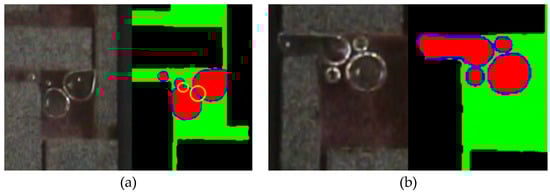
Figure 8.
Example of contacting bubble segmentation. (a) Incomplete segmentation, where neighboring bubbles are not fully separated (highlighted in orange). (b) Successful segmentation, where individual bubbles are distinctly identified. The comparison illustrates the challenge of accurately detecting and separating contacting bubbles during image analysis.
The correction of these artefacts can be performed in a straightforward manner with post-processing algorithms such as watershed separation, as the vast majority of the bubble border region is well defined. However, the use of image post-processing algorithms would need a thorough evaluation, as additional hyperparameters would have to be considered in the algorithm, and computing times would increase considerably with the number of bubbles captured in the frame. This evaluation is out of the scope of this study.
Regarding the tracking algorithm, the most demanding situation for the algorithm is when a bubble traverses a narrow channel of the porous medium, as depicted in Figure 9—bubble 2. Due to surface tension effects in combination with higher local fluid flow velocities, the bubble suffers an abrupt increase in velocity while traversing a narrow gap, which can be registered as a position jump by the video recording apparatus, due to an insufficient frame rate. Nevertheless, when a bubble reaches the end of a narrow gap (Figure 9—bubble 1), its velocity decreases again due to the stabilization of the fluid flow velocity, as well as the absence of significant bubble deformation and therefore surface tension forces. The combination of these effects is visible in Figure 10, where the plotted bubbles’ position parallel to the flow direction versus the corresponding video recording frame number may possess a “step”-like appearance, reflecting the differences in local velocities. Similarly, the flow-front position plot (dashed line) also possesses a “step”-like appearance due to the local higher fluid flow velocities in the narrow gaps of the porous medium. A total of twenty-five bubbles chosen randomly were plotted per experiment in Figure 10 to ease visualization.
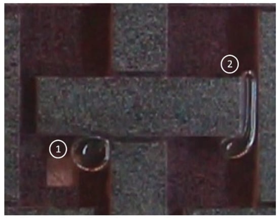
Figure 9.
Bubbles with different velocities: (1) bubble with low instantaneous velocity; (2) bubble with high instantaneous velocity.
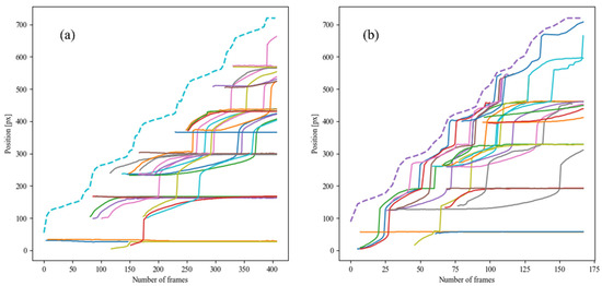
Figure 10.
Longitudinal position tracking results of bubbles (continuous lines, in different colors for easier visualization) and flow-front (dashed line) for (a) low flowrate experiment; (b) higher flowrate experiment.
The validation results demonstrate that the developed algorithm provides adequate segmentation and tracking performance on controlled 3D-printed geometries, providing a foundation for extension to more complex industrial applications. While real textile reinforcements with dual-scale porosity and irregular geometries will present additional challenges, the algorithm’s ability to handle different surface characteristics (SLA vs. MJF) and achieve acceptable error metrics suggests potential for adaptability. Future applications to varied manufacturing conditions would likely require targeted dataset expansion and potentially algorithm modifications, building upon the segmentation and tracking framework established in this study.
3.2. Flow-Front and Bubble Tracking Analysis
The bubble and flow-front tracking results presented in Figure 10 allow one to conclude that for this specific round of experiments, a higher flowrate and thus higher fluid flow velocity help promote a higher bubble velocity, which is in qualitative agreement with Bretherton’s theory [32].
Moreover, taking the two-dimensional tracking results of the bubbles’ trajectories depicted in Figure 11, it can be seen that the bubbles’ trajectories are not rectilinear but instead possess tortuosity, which is given by the porous medium geometry. Nevertheless, not all bubbles appear to be mobile, as a portion of the plotted bubbles maintain the same position throughout the entire video capture in both experiments. This phenomenon has been experimentally observed, as bubbles may become entrapped inside the structure of the porous medium, as the structures resembling fiber tows block the bubbles’ movement and the local fluid velocity is low there, stagnating the bubble. An example is provided in Figure 12, as the red dots represent the centroid position of the entrapped bubbles in an experiment. In light of this, modeling approaches of bubble transport processes in Liquid Composite Molding should also consider the stochastic dimension of these phenomena, aside from a purely deterministic framework.
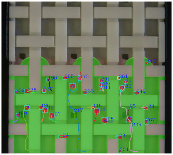
Figure 11.
Bubbles’ trajectory tracking results: tortuosity of the bubbles’ paths given by the porous medium architecture. Fluid highlighted in green, bubbles highlighted in red. Colored lines represent each bubble’s trajectory.
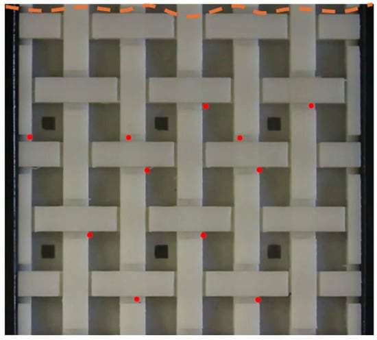
Figure 12.
Locations of entrapped bubbles during an experiment. The red markers indicate the positions where bubbles were observed within the porous structure, while the orange dashed line shows the flow-front at the corresponding time. This visualization highlights the relationship between bubble entrapment and the advancing flow-front.
Following the history of the bubble tracking results, depicted in Figure 13, it can be seen that there is significant bubble formation during the flow-front progression inside the porous medium. After the flow-front reaches the end of the porous medium, thus fully saturating it, bubble washout starts being the predominant phenomenon, whereby the number of bubbles reduces to less than half as the flow is allowed to bleed at the outlet. The number of bubbles tends to stabilize by the end of the experiment, where the entrapped bubbles are left inside the porous medium.
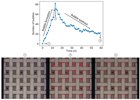
Figure 13.
Number of recorded bubbles (detected by the algorithm highlighted in red): (1) experiment start; (2) flow-front reaches end of porous medium; (3) end of experiment with steady-state flow at the outlet.
3.3. Bubble Transport Modelling
Through an analysis of the experiments described in Section 2.1, the results of which are detailed in [20], two pertinent dimensionless quantities were identified for describing void transport: The capillary number (), expressed in Equation (3), reflects the fluid flow conditions, which may impel the bubble further inside the porous medium by a buoyancy effect. The second number is the dimensionless bubble size (), which is the ratio between the bubble diameter and the porous medium representative hydraulic diameter (Equation (4)). This reflects the surface tension forces that may hinder or even stall bubble movement, as the fluid flow may not provide a drag force strong enough to squeeze the bubble through the porous medium constriction [20]. Therefore, as increases to one, bubbles benefit from increased buoyancy due to the increase in size. However, for values above one, bubbles need to be squeezed through the porous constrictions in order to move through the porous medium. As surface tension forces become predominant, bubble movement may be hindered.
Bubble mobility (), which is the ratio between bubble velocity () and volume average apparent fluid flow velocity (), as detailed in Equation (5), is a common dimensionless measure used in the literature to describe void transport efficiency [33]. Following this line of thought, bubble mobility should therefore be a result of the synergy between the former two dimensionless quantities.
To condense both capillary number and bubble size effects into a single variable, a dimensionless number is proposed () that reflects both the interactions between the capillary number and the non-dimensional bubble size, as expressed in Equation (6):
The square-root is used in the expression as a means of centering the experimental scattered data (geometrical mean) and has no physical significance, unlike and . This empirical combination was developed through systematic analysis of the experimental data to identify an effective correlation parameter that captures the interdependent effects of bubble size and flow conditions on bubble mobility, yielding the triangular distribution pattern observed in the results.
Given the scatterplot results presented in Figure 14, the resulting triangular-shaped pattern allows one to conclude that located at the apex of the triangle, there is a critical which separates two different tendencies: the bubble mobility increases with until it reaches the critical value , and then it continues to decrease.
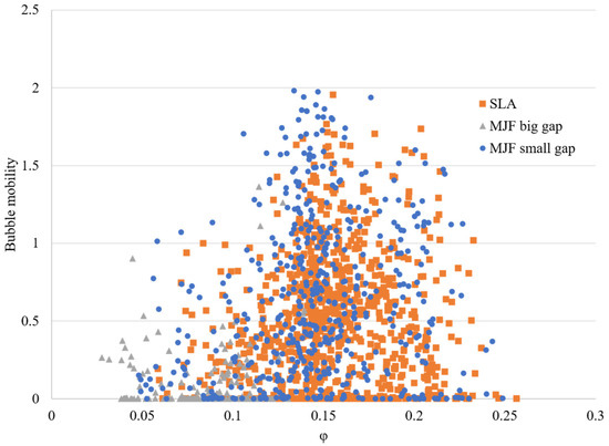
Figure 14.
Scatterplot of bubble mobility vs. non-dimensional number .
A more in-depth analysis of the data was conducted by dividing the scatterplot data into three different bins of equal size, thus taking advantage of the approximately symmetrical dataset. Hence, the first bin encompasses the left side of the suggested triangle, where a positive correlation between and bubble mobility is observed; the second bin encompasses the zone around the critical value; and the third bin encompasses the right side of the suggested triangle, where a negative correlation between and bubble mobility is observed. This data binning process can be seen in Figure 15.
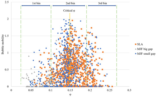
Figure 15.
Data binning process to explore correlation between and bubble mobility.
Having concluded the binning, data frequency measures were obtained for bubble mobility in each individual bin, and the respective histograms were computed (Figure 16). Moreover, for the ranges of for each bin, histograms were also computed for the corresponding flowrates and non-dimensional bubble sizes, presented in Figure 17 and Figure 18, respectively.
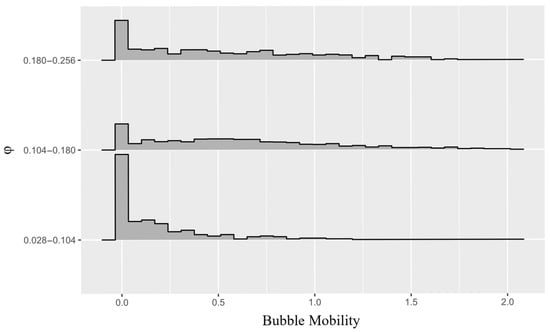
Figure 16.
Histogram plot of bubble mobility corresponding to each data bin.
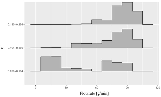
Figure 17.
Histogram plot of flowrate corresponding to each data bin.
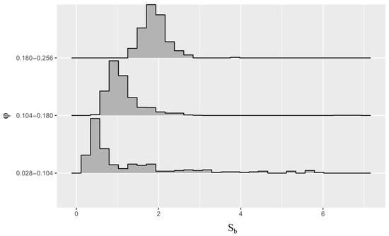
Figure 18.
Histogram plot of bubble non-dimensional size corresponding to each data bin.
Three different tendencies can be observed in each respective bin mobility histogram (Figure 16). In the first bin’s mobility histogram, although there are recorded values of bubble mobility above unity, the most probable scenario is the bubble mobility being close to null. A decreasing probability of increased bubble mobility is also observable. This is backed by the overall lower flowrates that are registered in this bin (Figure 17), associated with a broader distribution of bubble sizes (Figure 18). As described earlier, larger bubbles need an additional effort to be squeezed through the constriction, which in combination with a lower flowrate, greatly diminishes the probability of bubble mobility.
For the second bin, its bubble mobility histogram (Figure 16) presents two different modes, by which it is possible to conclude that there are two more probable scenarios: bubbles with a mobility close to null or bubbles with a mobility around 0.5. It is observable that in this bin, the distribution of non-dimensional bubble sizes is clustered around unity (Figure 18), which agrees with the above-stated physical principles. Hence, the scatter of the associated flowrates (Figure 17) should also contribute to the bubble mobility inflexion observed around the critical in Figure 15. At the inflexion point, there is also the maximum observed mobility, of around 2. This value is similar to the maximum bubble mobility value determined in other studies regarding void transport in LCM [33,34].
Finally, in the third bin’s histogram, it is possible to observe that the probability decreases with mobility (Figure 16), though this is less steep than in the first bin. The most probable scenario is still a bubble mobility close to null. Considering the third bin of , it is evident from Figure 18 that bubble sizes () tend to be larger than in the second bin. While the second bin is centered around one, it still falls within the middle of the range observed in the first bin. This suggests that as bubbles become larger than the gap size ( > 1), surface tension forces start to increase and consequently impede overall bubble mobility. This effect is observable in the scatterplot of Figure 15, where the envelope of bubble mobility takes a negative slope for values present in the third bin.
It is important to reinforce that zero mobility appears in all bins, since in all experiments there were bubbles which were formed in zones which did not provide any means for bubble movement. Moreover, as discussed in Section 3.2, throughout their trajectory, bubbles could become stagnant in one of those zones, therefore negatively impacting their mobility and contributing to the registered bubble mobility scatter.
It is important to note that while flow conditions (flowrates ranging from 10 g/min to 100 g/min) were systematically varied in this study, the bubble characteristics (size and number) could not be controlled independently, as all bubbles were generated naturally through flow-front mechanical air entrapment during mold filling. This means that the bubble mobility study presented represents the conditions naturally arising from the experimental setup and should not be regarded as a fully parametric study where bubble size and flow conditions could be varied independently. This natural generation approach, while limiting parametric control over bubble characteristics, provides a more realistic representation of void formation and transport mechanisms occurring in actual LCM processes [20].
4. Conclusions
In this study, a machine vision algorithm was successfully developed to detect and track both flow-front and bubble dynamics in Liquid Composite Molding using 3D-printed porous media. The U-Net-based segmentation model achieved low error rates in bubble detection and property estimation, demonstrating that effective monitoring is possible without elaborate experimental preparations such as fluid-coloring or complex lighting conditions. Coupling with tracking algorithms enabled comprehensive characterization of bubble transport efficiency throughout the injection process.
The experimental results revealed that bubble mobility is governed by both fluid flow conditions (capillary number) and geometrical considerations (bubble size relative to porous medium dimensions). A new dimensionless number () was proposed that effectively characterizes bubble transport efficiency, showing a critical value where bubble mobility transitions from increasing to decreasing behavior. Statistical analysis demonstrated distinct mobility distributions across different ranges, providing quantitative insights into void transport dynamics.
Key challenges identified include incomplete segmentation of contacting bubbles and the critical importance of adequate video frame rates for accurate tracking. Additionally, the simplified 3D-printed geometry, while enabling controlled experiments, represents an idealization of actual textile reinforcements that limits direct applicability to industrial LCM processes.
Future work will focus on extending this methodology to real dual-scale fibrous preforms and integrating thermal imaging to enhance segmentation robustness. The developed data-driven approach shows promise for enabling real-time process monitoring and control in actual LCM manufacturing, ultimately contributing to improved composite quality through better understanding and management of void formation and transport.
Author Contributions
Conceptualization, J.M. and M.B.; methodology, J.M., M.B. and S.A.; software, J.M.; validation, J.M., M.B. and S.A.; formal analysis, J.M. and M.B.; investigation, J.M. and M.B.; resources, M.B. and N.C.; data curation, J.M. and M.B.; writing—original draft preparation, J.M. and M.B.; writing—review and editing, S.A. and N.C.; visualization, J.M., M.B. and S.A.; supervision, N.C.; project administration, M.B. and N.C.; funding acquisition, M.B. and N.C. All authors have read and agreed to the published version of the manuscript.
Funding
J. Machado acknowledges the support from Agenda “Produzir Material Circulante Ferroviário em Portugal”, operation code 02-C05-i01.02-2022.PC645644454-00000065, financed by the Recovery and Resilience Plan (PRR) and by European Union—NextGeneration EU. S. Advani gratefully acknowledges the funding provided by the National Science Foundation Award No.2023323.
Data Availability Statement
The raw data supporting the conclusions of this article will be made available by the authors on request.
Conflicts of Interest
The authors declare no conflicts of interest.
Abbreviations
The following abbreviations are used in this manuscript:
| LCM | Liquid Composite Molding |
| SLA | Stereolithography |
| MJF | Multi-Jet fusion |
References
- Galvez-Hernandez, P.; Gaska, K.; Kratz, J. Phase segmentation of uncured prepreg X-Ray CT micrographs. Compos. Part A Appl. Sci. Manuf. 2021, 149, 106527. [Google Scholar] [CrossRef]
- Nguyen, D.; Davidson, P.; DeMille, K.; Ranatunga, V. Machine learning based segmentation of delamination patterns from sparse ultrasound data of barely visible impact damage in composites. J. Compos. Mater. 2025, 59, 321–330. [Google Scholar] [CrossRef]
- Meng, M.; Chua, Y.J.; Wouterson, E.; Ong, C.P.K. Ultrasonic signal classification and imaging system for composite materials via deep convolutional neural networks. Neurocomputing 2017, 257, 128–135. [Google Scholar] [CrossRef]
- Rudd, C.D.; Long, A.C.; Kendall, K.N.; Mangin, C.G.E. Liquid Moulding Technologies, 1st ed.; Woodhead Publishing Ltd.: Cambridge, UK, 1997. [Google Scholar]
- Arbter, R.; Beraud, J.M.; Binetruy, C.; Bizet, L.; Bréard, J.; Comas-Cardona, S.; Demaria, C.; Endruweit, A.; Ermanni, P.; Gommer, F.; et al. Experimental determination of the permeability of textiles: A benchmark exercise. Compos. Part A Appl. Sci. Manuf. 2011, 42, 1157–1168. [Google Scholar] [CrossRef]
- Konstantopoulos, S.; Hueber, C.; Antoniadis, I.; Summerscales, J.; Schledjewski, R. Liquid composite molding reproducibility in real-world production of fiber reinforced polymeric composites: A review of challenges and solutions. Adv. Manuf. Polym. Compos. Sci. 2019, 5, 85–99. [Google Scholar] [CrossRef]
- Agogué, R.; Shakoor, M.; Beauchêne, P.; Park, C.H. Analysis and Minimization of Race Tracking in the Resin-Transfer-Molding Process by Monte Carlo Simulation. Materials 2023, 16, 4438. [Google Scholar] [CrossRef]
- Fernández-León, J.; Keramati, K.; Garoz, D.; Baumela, L.; Miguel, C.; González, C. A Machine Learning Strategy for Race-Tracking Detection During Manufacturing of Composites by Liquid Moulding. Integr. Mater. Manuf. Innov. 2022, 11, 296–311. [Google Scholar] [CrossRef]
- Mehdikhani, M.; Gorbatikh, L.; Verpoest, I.; Lomov, S.V. Voids in fiber-reinforced polymer composites: A review on their formation, characteristics, and effects on mechanical performance. J. Compos. Mater. 2019, 53, 1579–1669. [Google Scholar] [CrossRef]
- Chai, B.X.; Eisenbart, B.; Nikzad, M.; Fox, B.; Blythe, A.; Blanchard, P.; Dahl, J. Simulation-based optimisation for injection configuration design of liquid composite moulding processes: A review. Compos. Part A Appl. Sci. Manuf. 2021, 149, 106540. [Google Scholar] [CrossRef]
- Park, M.; Tretyakov, M.V. Stochastic resin transfer molding process. SIAM-ASA J. Uncertain. Quantif. 2017, 5, 1110–1135. [Google Scholar] [CrossRef]
- Vollmer, M.; Zaremba, S.; Mertiny, P.; Drechsler, K. Edge race-tracking during film-sealed compression resin transfer molding. J. Compos. Sci. 2021, 5, 195. [Google Scholar] [CrossRef]
- Littner, L.; Protz, R.; Kunze, E.; Bernhardt, Y.; Kreutzbruck, M.; Gude, M. Flow Front Monitoring in High-Pressure Resin Transfer Molding Using Phased Array Ultrasonic Testing to Optimize Mold Filling Simulations. Materials 2024, 17, 207. [Google Scholar] [CrossRef] [PubMed]
- Nalla, A.R.; Fuqua, M.; Glancey, J.; Lelievre, B. A multi-segment injection line and real-time adaptive, model-based controller for vacuum assisted resin transfer molding. Compos. Part A Appl. Sci. Manuf. 2007, 38, 1058–1069. [Google Scholar] [CrossRef]
- Johnson, R.J.; Pitchumani, R. Simulation of active flow control based on localized preform heating in a VARTM process. Compos. Part A Appl. Sci. Manuf. 2006, 37, 1815–1830. [Google Scholar] [CrossRef]
- Lee, J.; Duhovic, M.; May, D.; Allen, T.; Kelly, P. Physics-informed neural networks for real-time simulation of transverse Liquid Composite Moulding processes and permeability measurements. Compos. Part A Appl. Sci. Manuf. 2025, 193, 108857. [Google Scholar] [CrossRef]
- Lee, D.; Lee, I.Y.; Park, Y.B. Real-time process monitoring and prediction of flow-front in resin transfer molding using electromechanical behavior and generative adversarial network. Compos. Part B Eng. 2025, 298, 112382. [Google Scholar] [CrossRef]
- LeBel, F.; Ruiz, É.; Trochu, F. Experimental study of saturation by visible light transmission in dual-scale fibrous reinforcements during composite manufacturing. J. Reinf. Plast. Compos. 2017, 36, 1693–1711. [Google Scholar] [CrossRef]
- Bodaghi, M.; Ban, D.; Mobin, M.; Park, C.H.; Lomov, S.V.; Nikzad, M. Additively manufactured three dimensional reference porous media for the calibration of permeability measurement set-ups. Compos. Part A Appl. Sci. Manuf. 2020, 139, 106119. [Google Scholar] [CrossRef]
- Machado, J.; Bodaghi, M.; Nikzad, M.; Camanho, P.P.; Advani, S.; Correia, N. On the understanding of bubble dynamics through a calibrated textile-like porous medium using a machine learning based algorithm. Compos. Part A Appl. Sci. Manuf. 2024, 177, 107955. [Google Scholar] [CrossRef]
- Bodaghi, M.; Mobin, M.; Ban, D.; Lomov, S.V.; Nikzad, M. Surface quality of printed porous materials for permeability rig calibration. Mater. Manuf. Process. 2021, 37, 548–558. [Google Scholar] [CrossRef]
- Ronneberger, O.; Fischer, P.; Brox, H. U-Net: Convolutional Networks for Biomedical Image Segmentation. In Proceedings of the Medical Image Computing and Computer-Assisted Intervention–MICCAI 2015, Munich, Germany, 5–9 October 2015; Volume 9351, pp. 234–241. [Google Scholar] [CrossRef]
- Srivastava, N.; Hinton, G.; Krizhevsky, A.; Sutskever, I.; Salakhutdinov, R. Dropout: A Simple Way to Prevent Neural Networks from Overfitting. J. Mach. Learn. Res. 2014, 5, 1929–1958. [Google Scholar]
- Abadi, M.; Agarwal, A.; Barham, P.; Brevdo, E.; Chen, Z.; Citro, C.; Corrado, G.S.; Davis, A.; Dean, J.; Devin, M.; et al. TensorFlow: Large-scale machine learning on heterogeneous systems. arXiv 2016, arXiv:1603.04467. [Google Scholar]
- Kingma, D.P.; Ba, J.L. Adam: A method for stochastic optimization. In Proceedings of the 3rd International Conference on Learning Representations, ICLR 2015, San Diego, CA, USA, 7–9 May 2015; pp. 1–15. [Google Scholar]
- Kervadec, H.; Bouchtiba, J.; Desrosiers, C.; Granger, E.; Dolz, J.; Ben Ayed, I. Boundary loss for highly unbalanced segmentation. Med. Image Anal. 2021, 67, 101851. [Google Scholar] [CrossRef] [PubMed]
- Bradski, G. The OpenCV Library. Dr. Dobb’s J. Softw. Tools Prof. Program. 2000, 25, 120–123. [Google Scholar]
- Liu, S.; Liu, D.; Srivastava, G.; Połap, D.; Woźniak, M. Overview and methods of correlation filter algorithms in object tracking. Complex Intell. Syst. 2021, 7, 1895–1917. [Google Scholar] [CrossRef]
- Bolme, D.; Beveridge, J.R.; Draper, B.A.; Lui, Y.M. Visual object tracking using adaptive correlation filters. In Proceedings of the 2010 IEEE Computer Society Conference on Computer Vision and Pattern Recognition, San Francisco, CA, USA, 13–18 June 2010; pp. 2544–2550. [Google Scholar] [CrossRef]
- Danelljan, M.; Häger, G.; Shahbaz Khan, F.; Felsberg, M. Accurate Scale Estimation for Robust Visual Tracking. In Proceedings of the British Machine Vision Conference 2014, Nottingham, UK, 1–5 September 2014; pp. 65.1–65.11. [Google Scholar] [CrossRef]
- King, D.E. Dlib-ml: A machine learning toolkit. J. Mach. Learn. Res. 2009, 10, 1755–1758. [Google Scholar]
- Bretherton, F.P. The motion of long bubbles in tubes. J. Fluid Mech. 1961, 10, 166. [Google Scholar] [CrossRef]
- Kang, K.; Koelling, K. Void transport in resin transfer molding. Polym. Compos. 2004, 25, 417–432. [Google Scholar] [CrossRef]
- Gangloff, J.J.; Hwang, W.R.; Advani, S.G. Characterization of bubble mobility in channel flow with fibrous porous media walls. Int. J. Multiph. Flow 2014, 60, 76–86. [Google Scholar] [CrossRef]
Disclaimer/Publisher’s Note: The statements, opinions and data contained in all publications are solely those of the individual author(s) and contributor(s) and not of MDPI and/or the editor(s). MDPI and/or the editor(s) disclaim responsibility for any injury to people or property resulting from any ideas, methods, instructions or products referred to in the content. |
© 2025 by the authors. Licensee MDPI, Basel, Switzerland. This article is an open access article distributed under the terms and conditions of the Creative Commons Attribution (CC BY) license (https://creativecommons.org/licenses/by/4.0/).