Article

Domain-Driven Teacher–Student Machine Learning Framework for Predicting Slope Stability Under Dry Conditions

by
Semachew Molla Kassa
1,2,
Betelhem Zewdu Wubineh
2,3,*,
Africa Mulumar Geremew
1,
Nandyala Darga Kumar
4 and
Grzegorz Kacprzak
5,*
1
Faculty of Civil and Water Resource Engineering, Bahir Dar Institute of Technology, Bahir Dar University, Bahir Dar P.O. Box 26, Ethiopia
2
College of Engineering and Technology, Wachemo University, Hossaena P.O. Box 667, Ethiopia
3
Faculty of Information and Communication Technology, Wroclaw University of Science and Technology, 50-370 Wroclaw, Poland
4
Hyderabad College of Engineering, Jawaharlal Nehru Technological University Hyderabad, Hyderabad 500085, India
5
Faculty of Civil Engineering, Warsaw University of Technology, 00-637 Warsaw, Poland
*
Authors to whom correspondence should be addressed.
Appl. Sci. 2025, 15(19), 10613; https://doi.org/10.3390/app151910613
Submission received: 15 September 2025 / Revised: 25 September 2025 / Accepted: 27 September 2025 / Published: 30 September 2025
(This article belongs to the Section Civil Engineering)

Abstract

Slope stability prediction is a critical task in geotechnical engineering, but machine learning (ML) models require large datasets, which are often costly and time-consuming to obtain. This study proposes a domain-driven teacher–student framework to overcome data limitations for predicting the dry factor of safety (FS dry). The teacher model, XGBoost, was trained on the original dataset to capture nonlinear relationships among key site-specific features (unit weight, cohesion, friction angle) and assign pseudo-labels to synthetic samples generated via domain-driven simulations. Six student models, random forest (RF), decision tree (DT), shallow artificial neural network (SNN), linear regression (LR), support vector regression (SVR), and K-nearest neighbors (KNN), were trained on the augmented dataset to approximate the teacher’s predictions. Models were evaluated using a train–test split and five-fold cross-validation. RF achieved the highest predictive accuracy, with an R2 of up to 0.9663 and low error metrics (MAE = 0.0233, RMSE = 0.0531), outperforming other student models. Integrating domain knowledge and synthetic data improved prediction reliability despite limited experimental datasets. The framework provides a robust and interpretable tool for slope stability assessment, supporting infrastructure safety in regions with sparse geotechnical data. Future work will expand the dataset with additional field and laboratory tests to further improve model performance.

1. Introduction

Landslides cause human losses and economic damage to infrastructure, including roads, railway lines, and agricultural and village areas. Slope stability analysis plays a positive role in protecting human lives and infrastructure by providing engineering mitigations that maintain natural conditions. The slope stability analysis is determined based on the strength of the soil materials, groundwater conditions, the angle of the ground, the matric suction of the soil conditions, and the surcharge applied to the slope. The uncertainty of these parameters also affects the stability of the hill [1,2]. Currently, climate change also hurts the stability of slopes. So, predicting the slope stability is still a challenge, especially due to the scarcity of data.
There are different methods of collecting input parameters for slope stability analysis, such as geophysical methods, geotechnical methods, and integration of both geophysical and geotechnical methods [3,4,5]. After collecting the input parameters, slope stability analysis methods are also physical-based, data-based, and the integration of the two methods [6,7]. Physical-based slope stability analyses are derived from the principles of soil mechanics and engineering geology. It is simply calculated by determining the mobilizing forces and the resisting forces [8,9]. Two-dimensional (2D) and three-dimensional (3D) slope stability analyses give different results, but the 3D slope stability analysis [10,11,12] considers the real problems because it considers the topographic conditions, groundwater conditions, and some tilt angles, which are not covered by the 2D slope stability analysis [13,14]. Previous researchers did not consider the effect of matric suction on the determination of the FS, both in the case of 2D and 3D slope stability analyses [15,16]. It has positive effects on the increase in factor safety during the dry season, but a negative effect during the rainy season. Recently, scholars have considered the effect of the matric suction effect on slope stability analysis, and it minimizes the material cost when it has a positive effect. Engineering assumptions also have some effects during the analysis of slope stability in 2D cases [17,18]. The climate parameters like temperature, rainfall, and snow also increase the slope instability problems, which lead to collapsed infrastructure during both seasons [19,20].
Data-driven methods provide an alternative approach to predicting slope stability [21,22,23]. Different machine learning (ML) algorithms can learn from training datasets obtained from field tests, laboratory experiments, and satellite data to predict slope stability problems. These methods perform well when the training data are of high quality and sufficiently large, although they may require significant computational time and resources [24,25,26]. Comparative studies of various ML techniques are often used to identify the most accurate predictive model. Additionally, results from laboratory tests and finite element (FE) analyses can be compared with ML predictions to validate their accuracy [27,28]. For example, in slope stability assessment, multilayer perceptron (MLP), decision tree (DT), and random forest (RF) models were evaluated for FS estimation, with MLP achieving the highest accuracy [29,30].
To improve prediction accuracy, increase the quality of the data and the amount of data. The geotechnical investigation, the number of boreholes, types of equipment used, and the skill of the drillers and collectors have effects on the accuracy of the prediction [7,31,32]. Several researchers tried to increase the amount of data to improve the accuracy of predictions [33,34]. Even as the amount of data increases, the accuracy of the prediction is not improved because of the ground conditions, such as the discontinuities of the layers, the types of soil, rock types, and the orientation of the soil fabrics [35,36]. Such training of ML models gives poor prediction results. Soils have different properties in the horizontal and vertical directions. This affects the strength parameters of the soil.
In addition to learning from historical slope cases, geotechnical engineering software was also used to generate simulated data to train the ML model. Researchers [37,38,39,40] generated 150 slope cases with pre-defined parameter ranges in OptumG2 simulation software, and then used these simulation data to train the ensemble classifier. Software like PLAXIS 2D, Rocscience 2D, and GeoStudio 2018 generate data to train the ML [41,42]. Numerical simulation should be based on historical data, laboratory tests, and field tests. Otherwise, it would lead to a false assessment of slope stability conditions.
In addition, there are also other types of analyses based on physical information and day-to-day monitoring information, like an inclinometer, extensometers, and piezometers for the measurement of vertical deformation, horizontal displacement, and groundwater condition measurements. If these data are integrated with the strength parameters of the soil, the accuracy of the prediction would be better [43]. The methods were followed and improved by [44]. Still, the challenges of slope stability are there in mountainous areas and are easily favorable for earthquake problems. The stratigraphic uncertainty and spatial variability of the soil also affect the accuracy of the prediction [45].
The research gap in the road corridor is limited in the use of modern ML or deep learning approaches, weak or small landslide inventory and temporal coverage, little rainfall trigger modeling, sparse in situ or geotechnical data and subsurface features, lack of spatial awareness validation and uncertainty quantification, class imbalance, sampling bias and scale/resolution mismatches, little integration of socioeconomic vulnerability, and impact or risk. Due to this gap, the corridor faces road failures during the rainy seasons from June to September.
In this study, the datasets were collected from geophysical and laboratory tests from the sections of the Bonga to Mizan road on the failed slope for the analysis of slope stability. To improve the accuracy of prediction, a multistage ML model is proposed. Hybrid ML models are also proposed to increase the efficiency of slope stability predictions. The developed model is compared with the previous prediction models and numerical simulation results. The proposed model is evaluated based on geotechnical laboratory investigation and the finite element methods.
In this study, the teacher–student learning framework is adopted to predict the slope stability under dry conditions. While teacher–student methods have been widely applied in computer science, their adaptation to geotechnical engineering requires additional considerations. The advantages of proposed approach are three-fold: (1) the teacher (XGBoost) captures complex nonlinear relationships and transfers knowledge to simpler student models; (2) student models such as RF and DT provide interpretable and computationally efficient alternatives for practitioners; and (3) synthetic data are generated using domain-driven Gaussian sampling constrained by geotechnical boundaries, ensuring physically meaningful augmentation compared with traditional methods. The main objectives of this study are to predict the stability analysis of the slope using deep learning and ML approaches, considering the geotechnical laboratory data, which are investigated by the Ethiopian Road Administration (ERA). The contributions of this study are as follows:
  • Collection of new geotechnical and field data, as well as site conditions, for analysis
  • Proposal of a domain-driven approach to artificially generate data to overcome data limitations
  • Training of a model using a teacher–student approach to achieve better results
  • Comparison of the performance of different ML approaches using various metrics, and selection of the best model for predicting safety factors.
This study aims to predict the factor of safety under dry conditions using the collected dataset. The scope of this study is limited to the road corridor from Bonga town to Mizan town, and it mainly relies on geotechnical and field tests. The significance of this research lies in its potential to minimize the time and effort required for designing landslide mitigation measures.

2. Materials and Methods

2.1. Data Preparation for Slope Stability Analysis

Various factors, including the angle of internal friction, cohesion, slope geometry, matric suction, unit weight of the soil, and pore water pressure, influence the stability of a slope. In this study, the angle of internal friction, cohesion, and unit weight were considered in determining the factor of safety for dry conditions (FS dry) for slope stability analysis. All attributes, except for the site, are continuous real numbers, while the site attribute is categorical. The site attribute was numerically labeled from 1 to 11 according to the section of the landslide, the station, and the location, as shown in Table 1. These labeled values correspond to specific site names, stations, and UTM coordinates, allowing for a structured representation of the categorical variable for modeling purposes. We collected a total of 300 records from the road corridor.
Where (γ) is the unit weight of the soil in kg/m3; (c) is cohesion in kN/m2; (ϕ) is the angle of internal friction in degrees, and FS is the factor of safety.
A total of 300 geotechnical laboratory records were collected from the Bonga–Mizan road corridor. Many of these records had identical FS dry values but slightly different measurements of unit weight, cohesion, and friction angle. To develop a clear and non-redundant dataset for machine learning, 22 unique FS dry records were selected as representatives of distinct slope stability conditions. Both the full 300-record dataset and the 22 unique-record subsets were tested in preliminary experiments using the proposed teacher–student framework. Results showed that the 22-record dataset, combined with domain-driven data augmentation, provided more robust and reliable model performance compared to using all 300 records, likely because the augmentation could focus on representative cases without redundancy. Using the 22 unique records as input, our domain-driven approach generated 800 synthetic samples while maintaining physically realistic feature ranges, creating a sufficiently large dataset for training and evaluating the student models. The sample FS is shown in Figure 1, where the horizontal axis represents the transversal direction of the road, and the vertical axis represents the depth of the soil layer.

2.2. Input Data from Geotechnical Tests

Data from both tests are useful for predicting slope stability. However, collecting large amounts of data is costly and requires considerable time, energy, and money. Machine learning methods generally need extensive datasets to achieve high accuracy in predicting the FS for a given area. Laboratory results are also used to validate the predictions generated by the ML algorithms.
Historical data is necessary from different published works and projects. From historical data, parameters such as unit weight of the soil, cohesion, and angle of friction are collected from slope stability published works, and the data help to explore and increase the accuracy of the model. In addition, PLAXIS 2D and Geo5 were used to generate data for this study, both of which support the prediction of slope stability. Table 2 provides a statistical summary of the soil parameters obtained from historical, numerical, geotechnical, and geophysical tests at the investigated sites. The table shows the mean, standard deviation, minimum, maximum, and quartile values of site, unit weight, cohesion, friction angle, and factor of safety under dry conditions (FS dry).
The correlation heatmap of the data set is presented in Figure 2. As observed, the friction angle is highly correlated with unit weight, and FS dry shows a strong correlation with cohesion, followed by the site attribute in the original data.
To ensure that the generated synthetic data is consistent with the original experimental dataset, we performed a validation of the augmented samples. The feature distributions of unit weight, cohesion, and friction angles in the synthetic dataset were compared with the original 22 unique FS dry records, and correlation analysis was conducted as shown in Figure 2. The results show that the synthetic data preserves the key relationships among features, including the negative correlation between cohesion and friction angle, while maintaining physically realistic bounds for all parameters. This validation confirms that the domain-driven synthetic data is suitable for training the student models and supports reliable FS dry predictions.
The distribution of the input parameters is illustrated in Figure 3 using box plots, where the horizontal axis represents the attribute, and the vertical axis represents the frequency of each value. These plots highlight the physical conditions of each slope, the variability of the parameters, and the presence of outliers. In a box plot, the bottom whisker represents the minimum value, and the lower edge of the box corresponds to the first quartile (25%); the line inside the box indicates the median (50%); the upper edge represents the third quartile (75%), and the top whisker shows the maximum value, excluding outliers (denoted as small circles). As shown in Figure 3, the median value of the site attribute is 6, which corresponds to the site Mizan-4, indicating that the middle portion of the dataset mainly comes from this landslide section. For unit weight and FS dry, some outliers are observed at the upper end of the distribution.
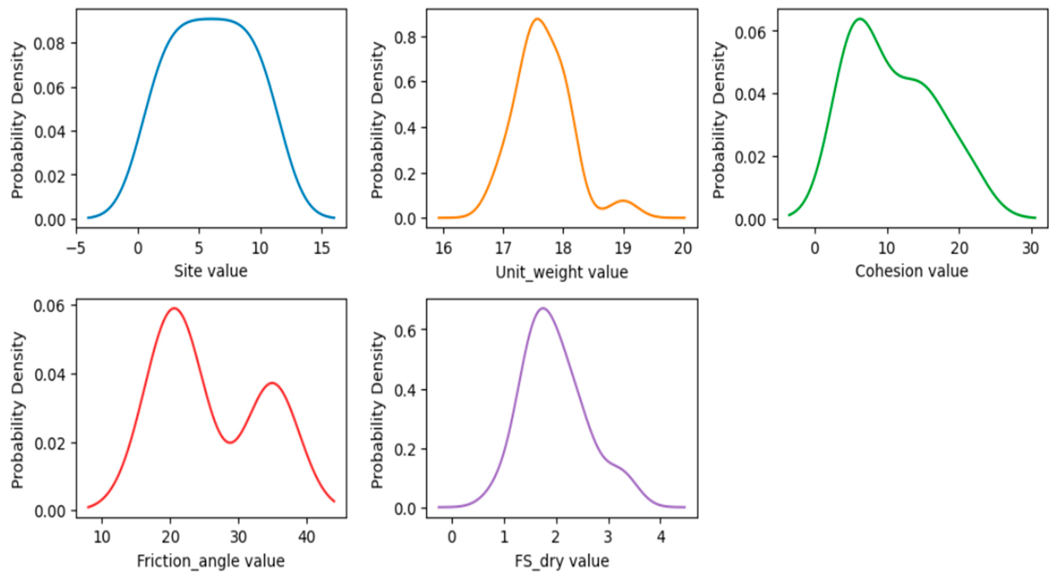
The overall distribution and patterns of the variables provide insight into the characteristics of the dataset, as depicted in Figure 4 using a density plot. As observed, the categorical variable site shows a roughly uniform distribution, indicating balanced sampling across landslide sites. Among continuous variables, unit weight is slightly right-skewed, reaching a peak around 17–18, while cohesion and friction angle exhibit bimodal distributions, suggesting the presence of distinct soil groups or site-specific conditions. FS dry, representing the factor of safety under dry conditions, is roughly unimodal, peaking near 2, which indicates that most slopes are moderately stable.
In general, the distributions highlight the variability in soil properties and slope characteristics throughout the study area.
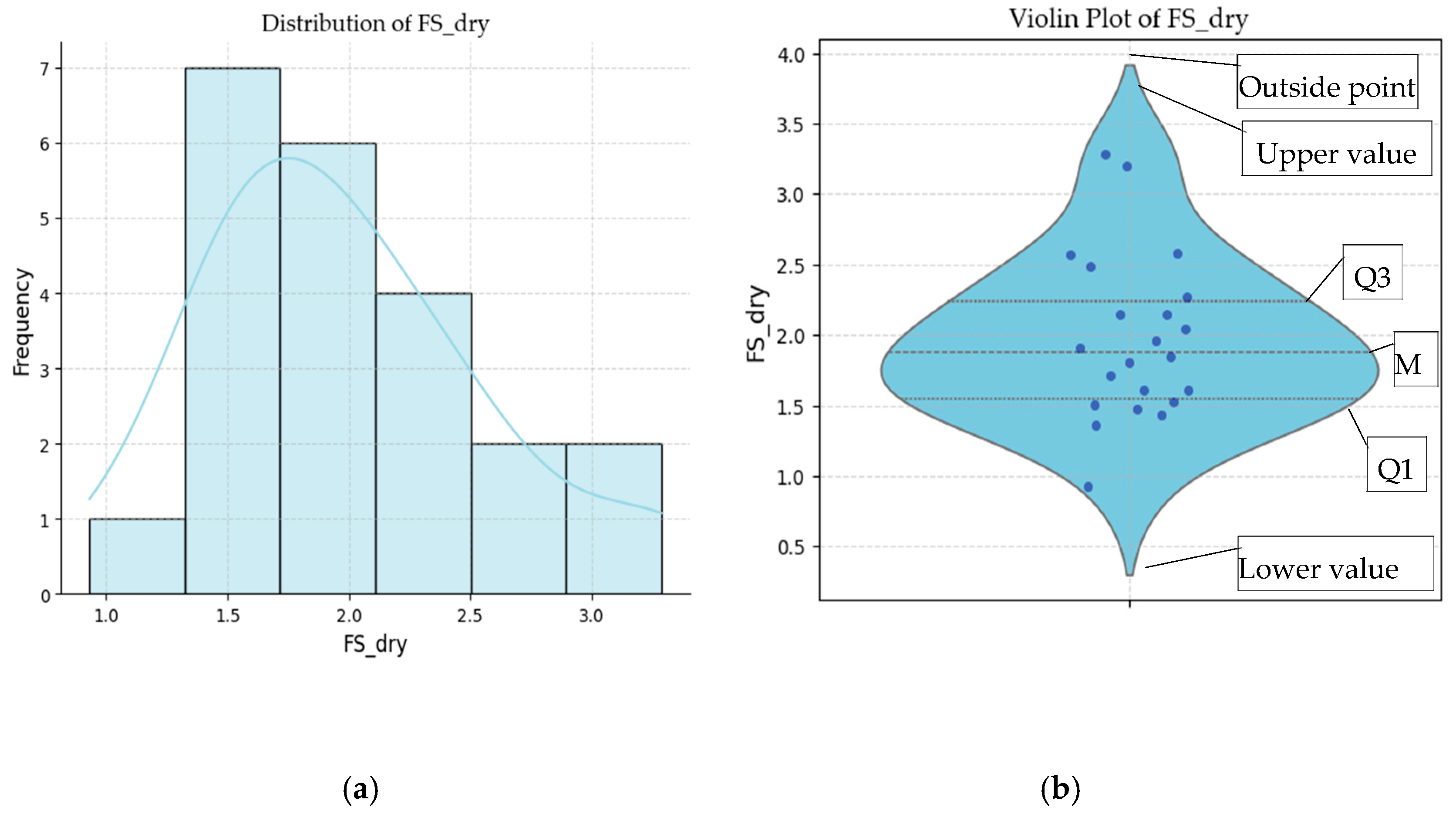
The distribution of FS dry is visualized using a histogram and a violin plot (Figure 5), showing the frequency of different factors of safety values under dry conditions. Most slopes have FS dry values between 1.5 and 2.0, with the highest frequency observed in the 1.5–1.7 range. Fewer slopes have higher values above 2.5, and very few slopes fall below 1.0, indicating that extremely unstable slopes are rare. Overall, the distribution is right-skewed, suggesting that most slopes are moderately stable, with a smaller number exhibiting higher safety factors.

2.3. Machine Learning Models

Machine learning models typically require a large amount of data for effective training. Because of the limited experimental data available, we propose a teacher–student domain-driven augmentation framework to improve the prediction of the dry factor of safety (FS dry). This is used to improve the performance of the model [46]. The teacher model, an XGBoost regressor, is trained on the original dataset to capture complex nonlinear relationships among the features (site, unit weight, cohesion, friction angle) and is used to assign pseudo-labels to synthetic samples generated via domain-driven simulation. Synthetic data are generated by sampling unit weight, cohesion, and friction angle from site-specific Gaussian distributions, with clipping applied to ensure values remain within physically realistic bounds. This process preserves the underlying correlations among features, as confirmed through correlation analysis (see Section 2.2 and Figure 2). The simulation produces realistic feature values by sampling from site-specific Gaussian distributions, with clipping applied to maintain physical bounds. These augmented samples, combined with the original data, are used to train six student models: RF, DT, shallow ANN, linear regression (LR), support vector regression (SVR), and K-nearest neighbors (KNN). Unlike standard data augmentation, which often generates samples without considering physical constraints, our domain-driven strategy ensures that synthetic data respects geotechnical boundaries (e.g., realistic cohesion, unit weight, and friction angle ranges). The teacher–student setup further enhances prediction by allowing complex models (teacher) to guide simpler and more interpretable models (students), providing engineers with both accuracy and practical usability. The student models aim to approximate the teacher’s predictions while offering different trade-offs in interpretability and computational complexity. The 22 unique FS dry records described in Section 2.1, together with 800 domain-driven synthetic samples, were used as input for the teacher–student framework to train the machine learning models.

2.3.1. XGBoost

The teacher model in our framework is XGBoost, an ensemble boosting algorithm that builds decision trees sequentially, with each tree correcting the errors of the previous algorithm [47]. It is an enhanced version of the gradient boosting decision tree (GBDT) algorithm, consisting of multiple decision trees, and is widely used for both classification and regression tasks [48]. This approach allows XGBoost to capture complex nonlinear relationships among features, such as site, unit weight, cohesion, and friction angle, which are critical for predicting the dry factor of safety (FS dry). Its regularization techniques help prevent overfitting [48], making it highly effective even with limited experimental data. In our framework, the XGBoost teacher model is trained on the original dataset and used to assign pseudo-labels to synthetic samples generated via domain-driven simulation, guiding the student models toward more accurate predictions.

2.3.2. Random Forest

It is a widely used supervised ensemble learning method applied to both classification and regression problems [49]. The random forest constructs multiple independent decision trees and combines their predictions by averaging [50,51]. This approach reduces the risk of overfitting compared to a single DT and improves generalization on unseen data [52]. It can capture nonlinear relationships among features and is robust to noise, making it suitable for predicting the dry factor of safety even with a limited dataset. Its structure also allows for some interpretability through feature importance measures, providing insight into which site-specific factors most influence slope stability.

2.3.3. Decision Tree

It is a simple and interpretable ML model that recursively splits the data based on feature thresholds to minimize prediction error [53]. Each split creates branches that lead to predictions, making it easy to visualize and understand the relationship between input features and the dry factor of safety (FS dry). Although highly interpretable, a single DT is prone to overfitting, especially with small datasets [54], and may not capture complex nonlinear interactions as effectively as ensemble models like RF or XGBoost.

2.3.4. Shallow Neural Network

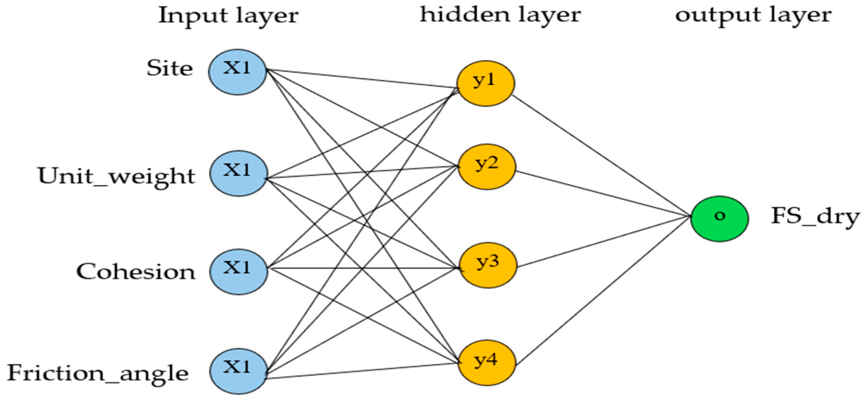
An ANN can learn patterns from data, associate new inputs with existing knowledge, and generate predictions while showing robustness to errors in the training set [55]. SNN is a neural network model with one hidden layer, capable of learning complex nonlinear relationships between input features and the target variable [56]. A sample SNN architecture is depicted in Figure 6. By adjusting the weights of connections between neurons during training, the ANN can model subtle patterns in the data, which is useful for predicting the dry factor of safety (FS dry). Although less interpretable than tree-based models, a shallow ANN requires less computational power than deep neural networks, making it suitable for small datasets while still capturing important nonlinear interactions among features.

2.3.5. Linear Regression

It is a simple and interpretable model that assumes a linear relationship between input features and the target variable [57], estimating the coefficients for each feature to best fit the observed data, making it easy to understand how each factor influences the dry factor of safety (FS dry). Although computationally efficient and straightforward, linear regression cannot capture complex nonlinear relationships, which may limit its predictive precision compared to more advanced models such as RF or ANN [58].

2.3.6. Support Vector Regression

It is a kernel-based ML model that aims to find a function that approximates the target values within a specified margin of tolerance [59]. Using kernel functions, SVR can capture nonlinear relationships between features and the dry factor of safety (FS dry), even in small datasets. It is effective at handling high-dimensional data and controlling overfitting [60], though it can be computationally intensive and less interpretable than simpler models like LR or a DT.

2.3.7. K-Nearest Neighbor

K-nearest neighbors (KNN) is a non-parametric, instance-based learning algorithm that predicts the output of a new sample based on the values of its K closest training samples [61]. It captures local patterns in the data, making it useful for modeling variations in the dry factor of safety (FS dry) across different sites. KNN is simple to implement and does not require explicit training, but it can be sensitive to noisy data and feature scaling, and its computational cost increases with the size of the dataset.
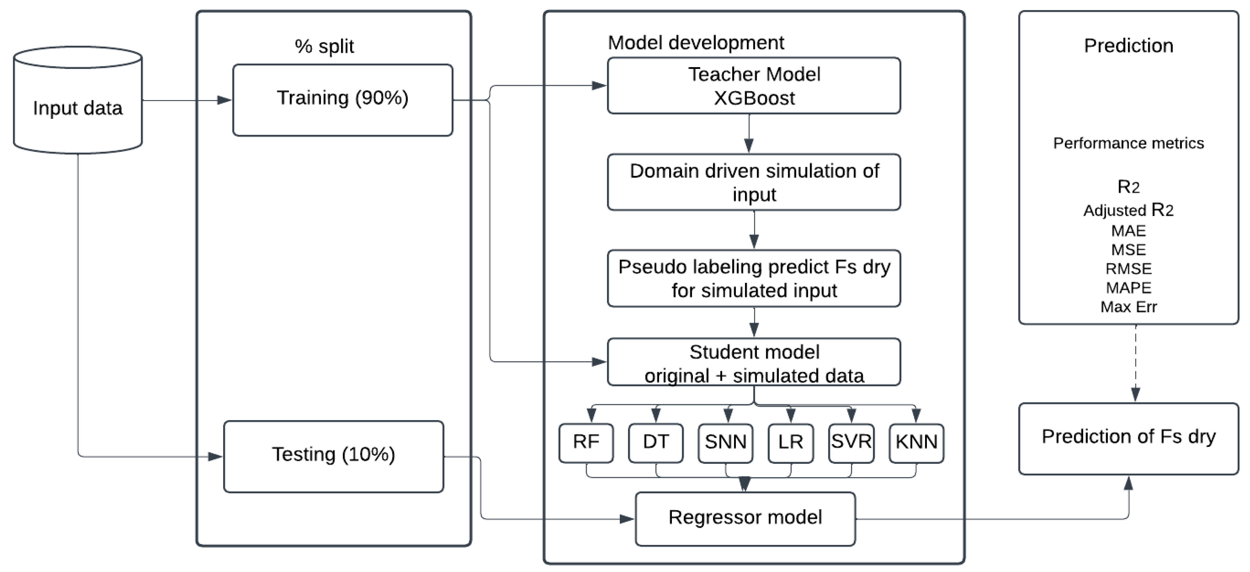
The flow of the proposed method is depicted in Figure 7. The proposed method follows a teacher–student knowledge transfer framework to improve the prediction of FS dry. Initially, the input dataset is split into training (90%) and testing (10%) sets. A teacher model (XGBoost) is trained in the original training data and used to simulate domain-driven inputs, generating pseudo-labeled data. This augmented dataset, combining original and simulated samples, is then used to train a student model. Various regression algorithms, including RF, DT, SNN, LR, SVR, and KNN, are applied to identify the best-performing predictor. The trained student model serves as a regressor for predicting FS dry on unseen testing data, and performance is evaluated using metrics such as R2, Adjusted R2, MAE, MSE, RMSE, MAPE, and Max Error. This approach leverages pseudo-labeling to enhance generalization and achieve more accurate predictions by integrating both real and simulated data.

2.4. Experimental Design and Evaluation Metrics

In this study, the dataset was divided into training and testing subsets using a 90:10 split, where 90% of the data was used to train the model, and the remaining 10% was reserved for testing its predictive performance. To ensure robustness, a 5-fold cross-validation strategy was also employed. In this approach, the training data is further divided into five subsets (folds), and the model is iteratively trained on four folds while validated on the remaining fold. This process is repeated five times, with each fold serving as the validation set once, and the performance metrics are averaged over all folds to provide a more reliable estimate of model generalization.
The performance of the model was evaluated using several commonly used regression metrics, including the coefficient of determination (R2), adjusted R2, mean absolute error (MAE), mean squared error (MSE), root mean squared error (RMSE), mean absolute percentage error (MAPE), and maximum error. These metrics provide complementary insights into the accuracy, reliability, and predictive performance of the model.
Coefficient of determination (R2): It measures how well a regression model explains the variability of the dependent variable (FS dry) based on the independent variables.
R 2 = 1 SS res SS tot
where
  • SSres = Residual sum of squares (unexplained variation);
  • SStot = Total sum of squares (total variation).
Adjusted coefficient of determination (Adjusted R2): It is a modified version of the coefficient of determination that penalizes the addition of unnecessary predictors in a regression model.
R adj 2 = 1 ( 1 R 2 ) * n 1 n p 1
where
  • n = number of data points (sample size);
  • P = number of predictors (independent variables);
  • R2 = coefficient of determination.
Maximum absolute error (MAE): It is a common statistical measure used to evaluate prediction accuracy in regression models or forecasting.
MAE = 1 n i = 1 n | y i y Ù |
where n = number of observations; y i = actual (true) value; | y i y i | = predicted value, and | y i y i | is an absolute error for each prediction.
Mean squared error (MSE): It is another commonly used error metric in statistics and ML, especially for regression and prediction tasks.
MSE = 1 n i = 1 n ( y i y i Ù ) 2
where n = number of observations; y i = actual (true) value; y i = predicted value, and ( y i y i ) 2 = squared error for each prediction.
Root mean squared error (RMSE): It is the square root of the mean squared error (MSE) and is one of the most widely used metrics for evaluating regression models.
RMSE = 1 n i = n n ( y i y Ù i ) 2
where n = number of observations; y i = actual (true) value; y i = predicted value, and ( y i y i ) 2 squared error.
Mean absolute percentage error (MAPE): It is a metric used to measure prediction accuracy in regression and forecasting by expressing the error as a percentage of the actual values.
MAPE = 100 n i = 1 n | y i y Ù i y i |
where n = number of observations; y i = actual (true) value; y i = predicted value.
Maximum error (Max Error): Maximum error (Max Error) is a regression metric that measures the largest single error between a predicted value and the actual value.
Max   Error = max i = 1 n | y i y Ù i |
where y i = actual (true) value; y i = predicted value, and | y i y i | = absolute error for each observation.
The hyperparameters for the teacher and student algorithms are shown in Table 3. To develop this experiment, we used the Python 3.11 programming language due to its versatility and wide range of libraries for ML and data analysis. Python efficiently facilitated data preprocessing, implementation of ML models, cross-validation, and performance evaluation.

3. Results

This section presents the results of this study, which aims to predict the FS under dry conditions in slope stability. Training data were obtained from both laboratory experiments and numerical simulations. The dataset was divided into 90% for training and 10% for testing, and a five-fold cross-validation technique was employed to ensure robust model evaluation. Various ML algorithms were used to predict slope stability: XGBoost as the teacher model, and RF, DT, SNN, LR, SCR, and KNN as student models in a domain-driven approach for generating artificial data. The results obtained using the train–test split are summarized in Table 4.
In Table 4, using the train–test split, the RF model achieved the highest predictive performance, with an R2 of 0.9663, an adjusted R2 of 0.9600, and the lowest error values (MAE = 0.0233, RMSE = 0.0531, and MAPE = 0.0116). Decision tree and SNN models also showed good performance but were slightly less accurate than RF. LR, SVR, and KNN exhibited comparatively lower predictive accuracy, with R2 values below 0.76 and higher error metrics. The result of this study using the five-fold cross-validation is shown in Table 5.
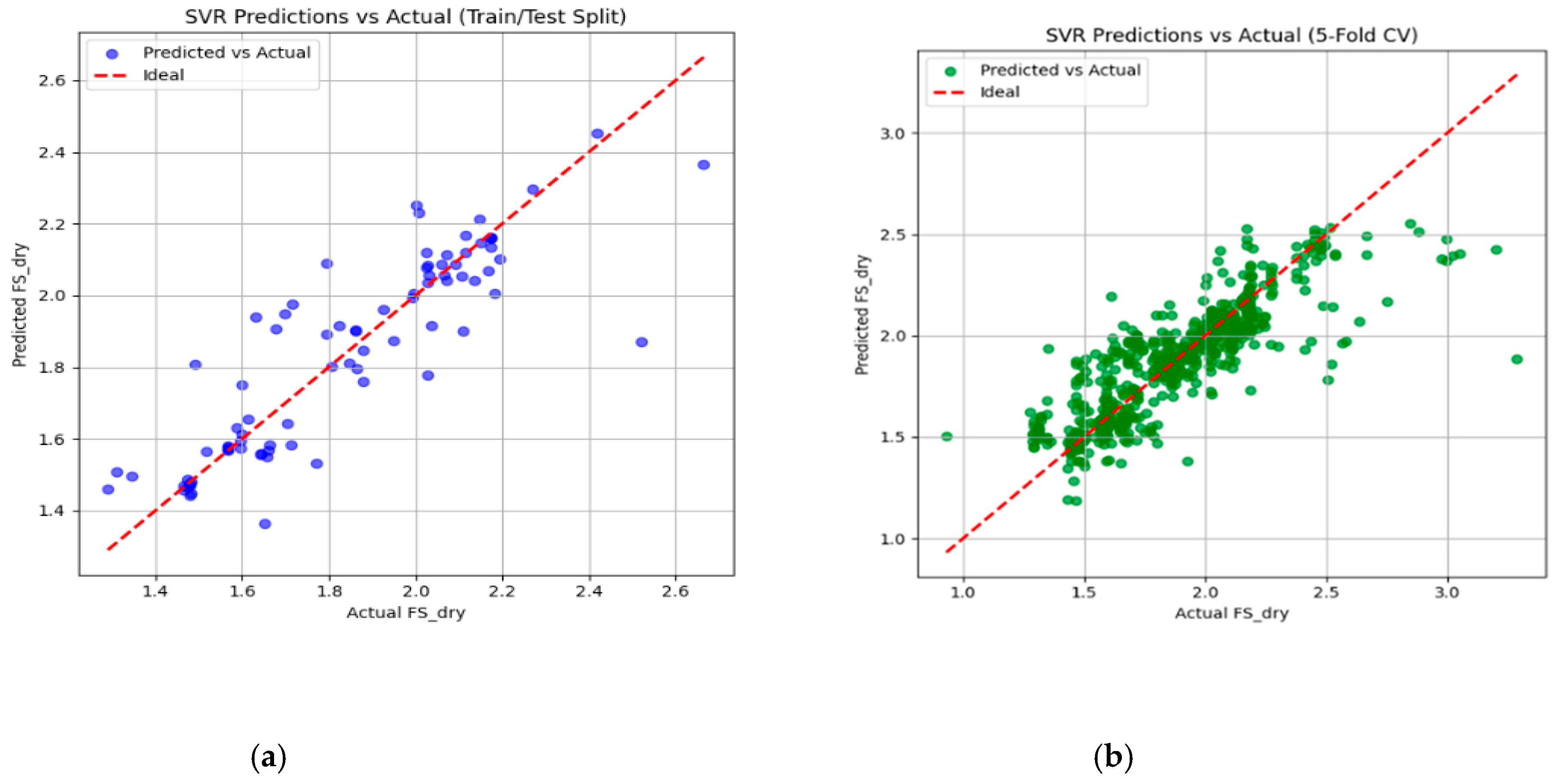
As can be seen in Table 5, the results of the five-fold cross-validation showed similar trends, with RF remaining the model that performed the best (R2 = 0.9281, adjusted R2 = 0.9269). Some models, such as DT and SNN, maintained good performance, while LR, SVR, and KNN showed lower predictive accuracy. The maximum errors were generally higher in cross-validation compared to the simple train–test split, indicating that some predictions deviated more from the actual values when the models were tested in multiple subsets. The comparison of results in the train–test split is shown in Figure 8. The SVR result of the split test train is depicted in Figure 9.
The SVR predictions for FS dry demonstrate a strong positive correlation with actual values in both the train–test split (a) and the five-fold cross-validation (b). In both plots, most of the points align closely with the diagonal red line, showing that the model captures the overall trend effectively. However, some scatter and deviations indicate occasional under- or over-predictions, especially at the extremes of the range. The cross-validation plot (b) reinforces the consistency of the model across folds, with predictions generally reliable between 1.4 and 2.6 FS dry, although outliers near the boundaries suggest harder cases. Importantly, these predicted values are directly compared with experimental laboratory measurements from the corresponding field locations, demonstrating that the machine learning-derived FS dry values closely match the observed data and validating the predictive accuracy. Overall, the SVR shows good predictive performance with room for improvement through hyperparameter tuning, feature engineering, or addressing data sparsity.

4. Discussions

The primary objective of this study was to predict the factor of safety under dry conditions (FS dry) for slopes using a domain-driven ML framework. The combination of a teacher–student augmentation approach and domain-driven synthetic data generation allowed us to overcome the limitation of small experimental datasets, which is a common challenge in geotechnical studies.
Our results demonstrated that RF consistently outperformed other student models across both the 90:10 train–test split and five-fold cross-validation. Specifically, RF achieved an R2 of 0.9663 in the train–test split and 0.9281 in the 5-fold CV, with the lowest error metrics (MAE, RMSE, MAPE). These results indicate that the RF model accurately captured the nonlinear relationships among site-specific variables (site, unit weight, cohesion, and friction angle) and the FS. Decision tree and shallow neural network (SNN) also performed well but were slightly less accurate, highlighting the advantage of ensemble methods like RF in capturing complex interactions and reducing overfitting. Linear regression, SVR, and KNN showed comparatively lower performance, likely due to their limited ability to capture complex nonlinear patterns in small datasets. The use of five-fold cross-validation further strengthened our findings by providing a robust estimate of model generalization. While some metrics (e.g., maximum error) were slightly higher under cross-validation, the overall trends remained consistent, indicating the reliability of the proposed methodology.
To ensure that the high predictive performance of the RF and XGBoost models was not due to overfitting, several measures were implemented. First, model evaluation was conducted using both a 90:10 train–test split and five-fold cross-validation, with the RF model achieving R2 = 0.9663 on the train–test split and R2 = 0.9281 on cross-validation, indicating good generalization. Second, hyperparameters were carefully selected to balance model complexity and bias–variance trade-off (Table 3). For RF, 300 trees were used with no maximum depth restriction but a minimum of two samples per split and one per leaf; for XGBoost, regularization (reg_lambda = 1.0), subsampling (0.9), and column sampling (0.9) were applied. These settings, combined with the domain-driven data augmentation, reduced the likelihood of overfitting while maintaining accurate predictions.
One of the key strengths of this study is the integration of domain knowledge into data augmentation. Using site-specific Gaussian sampling and clipping to maintain physically realistic values, we generated synthetic data that closely resembles real-world conditions. The XGBoost teacher model efficiently captured complex nonlinear relationships and provided pseudo-labels for these synthetic samples, guiding the student models toward higher predictive accuracy. This approach mitigates the common problem of small datasets in slope stability studies, which typically limits the performance of conventional ML models. Additionally, the framework allows for flexibility in model selection: tree-based models (RF, DT) benefit from ensemble learning and interpretability, neural networks (SNN) capture subtle nonlinear interactions, while linear and kernel-based models (LR, SVR) provide complementary perspectives. The combination ensures robust and reliable predictions across different ML paradigms.
An important consideration in synthetic data generation is whether the augmented samples preserve the physical relationships among soil parameters. In the original dataset, cohesion and internal friction angle exhibited a strong negative correlation (–0.838). We verified that the synthetic data maintained this negative dependency and preserved the overall correlation structure of the original dataset, while domain-driven clipping ensured that all values remained within realistic ranges. Nonetheless, we acknowledge that Gaussian sampling provides an idealized approximation and may not fully capture rare nonlinear dependencies. Future work could address this by adopting multivariate sampling or generative approaches (e.g., generative adversarial networks, GANs) to better preserve complex parameter interactions.
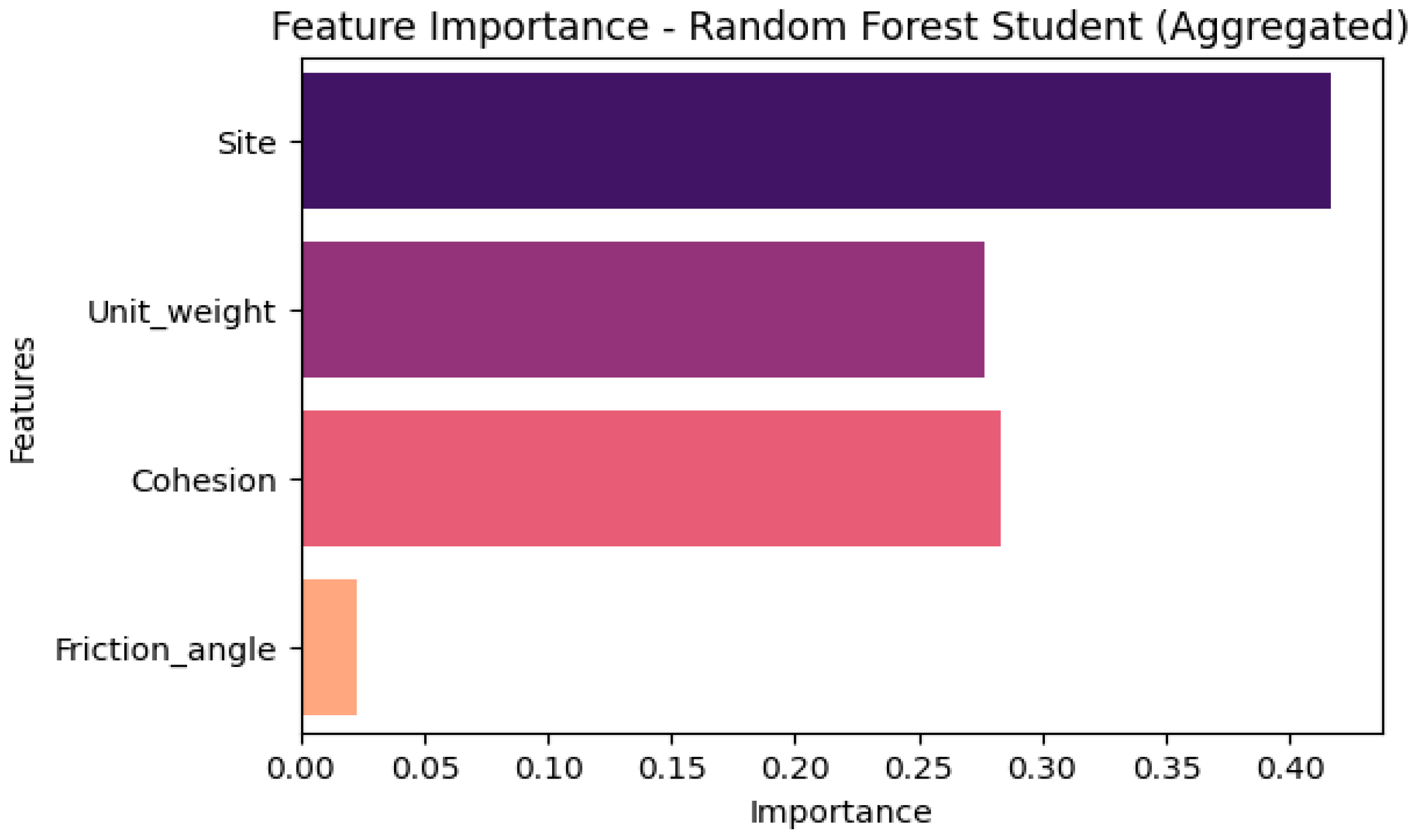
To better understand the contributions of individual parameters, an aggregated feature importance analysis was performed for the RF Student model. All one-hot encoded site variables were combined into a single “site” feature. The resulting feature importances are site (0.416), cohesion (0.284), unit weight (0.277), and friction angle (0.023). These results indicate that site information, cohesion, and unit weight are the most influential factors for predicting FS dry, while friction angles play a minor role. Figure 10 shows the corresponding feature importance graph, where the horizontal axis represents the value of the attribute importance, and the vertical axis represents the name of the attribute. This analysis enhances interpretability by highlighting the key geotechnical parameters driving slope stability predictions. A comparison of our study with previous work is presented in Table 6.
Table 6 presents a comparison of our random forest (RF) model with previously published regression-based studies for slope stability prediction. Our model, trained on 822 data points from Ethiopia, achieved the highest predictive performance across all reported metrics, with R2 = 0.9663, MAE = 0.0233, MSE = 0.0028, RMSE = 0.0531, and MAPE = 0.0116. Compared to other studies, including SVM, DT, and RF models in China [62] (R2 up to 0.8640), GPR and DT in Iran [63] (R2 up to 0.8139), linear regression in Vietnam and other countries [8] (R2 = 0.9265), and ANN/LSTM models [64,65] (R2 = 0.698–0.810), our approach demonstrates clearly superior accuracy and lower errors.
This enhanced performance can be attributed to the teacher–student domain-driven augmentation framework, which enriches the training data with high-quality pseudo-labeled samples while preserving realistic physical relationships among soil parameters. By integrating domain knowledge into synthetic data generation, the model captures complex nonlinear interactions between slope and soil features more effectively than conventional regression approaches. Consequently, our RF model not only achieves higher accuracy but also maintains interpretability through feature importance analysis and benefits from its ensemble approach, making it particularly suitable for practical slope stability assessments in regions with limited experimental or historical data.
The high predictive performance of the RF and DT models suggests that the proposed framework can be applied to real-world slope stability assessments, particularly in regions where experimental or historical data are limited. By combining physical understanding with ML, this methodology provides both accurate predictions and interpretable insights into the influence of key soil parameters (cohesion, friction angle, unit weight) on slope stability. Practitioners can use these models to prioritize slopes for monitoring or intervention, potentially reducing the risk of landslide events.
Although the results are promising, this study has limitations. Synthetic data generation relies on the assumption of Gaussian distributions for site-specific parameters, which may not fully capture extreme values or rare events, potentially affecting the generalization ability of the model to unseen slopes. Future work could explore non-Gaussian or conditional generative models to enhance the realism of synthetic data. Additionally, extending the framework to incorporate pore water pressure, matrix suction, slope geometry, temperature, rainfall, elevation, and aspect into the ML algorithm could improve prediction accuracy under variable environmental conditions. While the proposed teacher–student framework is computationally efficient for small to moderate datasets, larger datasets or more complex models (e.g., deep neural networks or hybrid ensemble models) could increase computational cost. Advanced ML and deep learning algorithms, including deep neural networks, gradient boosting variants (LightGBM, CatBoost), and hybrid ensemble models, could further improve predictive performance and robustness, especially with larger datasets.

5. Conclusions

In the application of machine learning (ML) for predicting slope stability in the selected area, challenges arise in collecting sufficient data to train the model. Geotechnical investigations require significant resources, including money, time, and energy, to gather datasets. Alternatively, instead of conducting new field and laboratory tests, collecting secondary data from previous studies and government-funded large projects can be more efficient.
The size of the training data, the quality of tests, and the equipment used also affect the prediction accuracy of the model. This study compiles training data from geotechnical laboratory tests, geophysical tests, historical data, and numerical simulations. The proposed model was evaluated using landslide cases from the Bonga–Mizan road corridor as well as data from the published literature.
To address the shortage of data, a domain-driven approach was used, with XGBoost as the teacher and RF, DT, SNN, LR, SVR, and KNN as student models to train the ML framework. Among these, RF was identified as the best algorithm for predicting the factor of safety. Future work will explore additional ML models to further improve prediction performance.

Author Contributions

Conceptualization, S.M.K., B.Z.W., A.M.G., N.D.K., and G.K.; methodology, S.M.K., B.Z.W., A.M.G., N.D.K., and G.K.; software, S.M.K. and B.Z.W.; validation, S.M.K., B.Z.W., A.M.G., N.D.K., and G.K.; data curation, S.M.K.; writing—original draft preparation, S.M.K. and B.Z.W.; writing—review and editing, S.M.K., B.Z.W., A.M.G., N.D.K., and G.K.; visualization, S.M.K. and B.Z.W.; supervision, A.M.G., N.D.K., and GK. All authors have read and agreed to the published version of the manuscript.

Funding

This research received no external funding.

Institutional Review Board Statement

Not applicable.

Informed Consent Statement

Not applicable.

Data Availability Statement

The data used to support the findings of this study are available from the corresponding author upon request.

Acknowledgments

We acknowledge the Ethiopian Road Administration and STrIDE Consulting Engineers PLC.

Conflicts of Interest

The authors declare no conflicts of interest.

References

  1. Chen, Y.; Kong, J.; Lou, Y.; Zhang, X.; Li, J.; Ling, D. Slope Stability Prediction Using Multi-Stage Machine Learning with Multi-Source Data Integration Strategy. Can. Geotech. J. 2025, 62, 1–18. [Google Scholar] [CrossRef]
  2. Bui, X.N.; Muazu, M.A.; Nguyen, H. Optimizing Levenberg–Marquardt Backpropagation Technique in Predicting Factor of Safety of Slopes after Two-Dimensional OptumG2 Analysis. Eng. Comput. 2020, 36, 941–952. [Google Scholar] [CrossRef]
  3. Frydrych, M.; Kacprzak, G.; Nowak, P. Hazard Reduction in Deep Excavations Execution. Sustainability 2022, 14, 868. [Google Scholar] [CrossRef]
  4. Kacprzak, G.; Frydrych, M.; Nowak, P. Influence of Load–Settlement Relationship of Intermediate Foundation Pile Group on Numerical Analysis of a Skyscraper under Construction. Sustainability 2023, 15, 3902. [Google Scholar] [CrossRef]
  5. Kacprzak, G.; Zbiciak, A.; Józefiak, K.; Nowak, P.; Frydrych, M. One-Dimensional Computational Model of Gyttja Clay for Settlement Prediction. Sustainability 2023, 15, 1759. [Google Scholar] [CrossRef]
  6. Yadav, D.K.; Chattopadhyay, S.; Tripathy, D.P.; Mishra, P.; Singh, P. Enhanced Slope Stability Prediction Using Ensemble Machine Learning Techniques. Sci. Rep. 2025, 15, 7302. [Google Scholar] [CrossRef] [PubMed]
  7. Moayedi, H.; Bui, D.T.; Kalantar, B.; Foong, L.K. Machine-Learning-Based Classification Approaches toward Recognizing Slope Stability Failure. Appl. Sci. 2019, 9, 4638. [Google Scholar] [CrossRef]
  8. Bui, D.T.; Moayedi, H.; Gör, M.; Jaafari, A.; Foong, L.K. Predicting Slope Stability Failure through Machine Learning Paradigms. ISPRS Int. J. Geo-Inf. 2019, 8, 395. [Google Scholar] [CrossRef]
  9. Pei, T.; Qiu, T.; Shen, C. Applying Knowledge-Guided Machine Learning to Slope Stability Prediction. J. Geotech. Geoenviron. Eng. 2023, 149, 127850. [Google Scholar] [CrossRef]
  10. Kacprzak, G.M.; Kassa, S.M. Assessment of the Interaction of the Combined Piled Raft Foundation Elements Based on Long-Term Measurements. Sensors 2025, 25, 3460. [Google Scholar] [CrossRef]
  11. Molla Kassa, S. A Systematic Review of Machine Learning Based Landslide Susceptibility Mapping. Put I Saob. 2024, 70, 23–30. [Google Scholar] [CrossRef]
  12. Molla Kassa, S.; Tamirat, H.; Quezon, E. Empirical Correlation of Hossaena Town Soil Index Properties with California Bearing Ratio (CBR) Values. Put I Saob. 2024, 70, 1–8. [Google Scholar] [CrossRef]
  13. Anuragi, S.K.; Kishan, D. Analysis Grid Search Optimization of Machine Learning Models for Slope Stability Prediction Supports the Design Construction of Geotechnical Structures and Environmental Development. Metall. Mater. Eng. 2025, 31, 260–273. [Google Scholar] [CrossRef]
  14. Zhang, Z.; Huang, J.; Su, Q.; Liu, S.; Mangi, N.; Zhang, Q.; Zhang, A.A.; Liu, Y.; Wang, S. High Embankment Slope Stability Prediction Using Data Augmentation and Explainable Ensemble Learning. Comput. Civ. Infrastruct. Eng. 2025, 40, 2833–2858. [Google Scholar] [CrossRef]
  15. Kurnaz, T.F.; Erden, C.; Dağdeviren, U.; Demir, A.S.; Kökçam, A.H. Comparison of Machine Learning Algorithms for Slope Stability Prediction Using an Automated Machine Learning Approach. Nat. Hazards 2024, 120, 6991–7014. [Google Scholar] [CrossRef]
  16. Gladious, J.; Paul, P.S.; Mukhopadhyay, M. Machine Learning Based Prediction of Geotechnical Parameters Affecting Slope Stability in Open-Pit Iron Ore Mines in High Precipitation Zone. Sci. Rep. 2025, 15, 21868. [Google Scholar] [CrossRef]
  17. Onyelowe, K.C.; Moghal, A.A.B.; Ahmad, F.; Rehman, A.U.; Hanandeh, S. Numerical Model of Debris Flow Susceptibility Using Slope Stability Failure Machine Learning Prediction with Metaheuristic Techniques Trained with Different Algorithms. Sci. Rep. 2024, 14, 19562. [Google Scholar] [CrossRef]
  18. Bai, G.; Hou, Y.; Wan, B.; An, N.; Yan, Y.; Tang, Z.; Yan, M.; Zhang, Y.; Sun, D. Performance Evaluation and Engineering Verification of Machine Learning Based Prediction Models for Slope Stability. Appl. Sci. 2022, 12, 7890. [Google Scholar] [CrossRef]
  19. Fu, X.; Zhang, B.; Wang, L.; Wei, Y.; Leng, Y.; Dang, J. Stability Prediction for Soil-Rock Mixture Slopes Based on a Novel Ensemble Learning Model. Front. Earth Sci. 2023, 10, 1102802. [Google Scholar] [CrossRef]
  20. Deris, A.M.; Solemon, B.; Omar, R.C. A Comparative Study of Supervised Machine Learning Approaches for Slope Failure Production. E3S Web Conf. 2021, 325, 01001. [Google Scholar] [CrossRef]
  21. Chauhan, V.S.; Sadique, M.R.; Alam, M.M.; Farooqi, M.A. Assessment of Road-Cut Slope Stability Using Empirical, Numerical, and Machine Learning Methodologies. Discov. Civ. Eng. 2025, 2, 108. [Google Scholar] [CrossRef]
  22. Han, Y.; Semnani, S.J. Integration of Physics-Based and Data-Driven Approaches for Landslide Susceptibility Assessment. Int. J. Numer. Anal. Methods Geomech. 2025, 49, 3060–3097. [Google Scholar] [CrossRef]
  23. Gao, W.; Zang, M.; Mei, G. Exploring Influence of Groundwater and Lithology on Data-Driven Stability Prediction of Soil Slopes Using Explainable Machine Learning: A Case Study. Bull. Eng. Geol. Environ. 2024, 83, 2. [Google Scholar] [CrossRef]
  24. Nanehkaran, Y.A.; Licai, Z.; Chengyong, J.; Chen, J.; Anwar, S.; Azarafza, M.; Derakhshani, R. Comparative Analysis for Slope Stability by Using Machine Learning Methods. Appl. Sci. 2023, 13, 1555. [Google Scholar] [CrossRef]
  25. Ragam, P.; Kushal Kumar, N.; Ajith, J.E.; Karthik, G.; Himanshu, V.K.; Sree Machupalli, D.; Ramesh Murlidhar, B. Estimation of Slope Stability Using Ensemble-Based Hybrid Machine Learning Approaches. Front. Mater. 2024, 11, 1330609. [Google Scholar] [CrossRef]
  26. Kardani, N.; Zhou, A.; Nazem, M.; Shen, S.L. Improved Prediction of Slope Stability Using a Hybrid Stacking Ensemble Method Based on Finite Element Analysis and Field Data. J. Rock Mech. Geotech. Eng. 2021, 13, 188–201. [Google Scholar] [CrossRef]
  27. Shakya, S.; Schmüdderich, C.; Machaček, J.; Prada-Sarmiento, L.F.; Wichtmann, T. Influence of Sampling Methods on the Accuracy of Machine Learning Predictions Used for Strain-Dependent Slope Stability. Geosciences 2024, 14, 44. [Google Scholar] [CrossRef]
  28. Mamat, R.C.; Ramli, A.; Samad, A.M.; Kasa, A.; Fatin, S.; Razali, M. Performance Prediction Evaluation of Machine Learning Models for Slope Stability Analysis: A Comparison Between ANN, ANN-ICA and ANFIS. J. Electr. Syst. 2024, 20, 4364–4374. [Google Scholar]
  29. Xi, N.; Yang, Q.; Sun, Y.; Mei, G. Machine Learning Approaches for Slope Deformation Prediction Based on Monitored Time-Series Displacement Data: A Comparative Investigation. Appl. Sci. 2023, 13, 4677. [Google Scholar] [CrossRef]
  30. Xu, H.; He, X.; Shan, F.; Niu, G.; Sheng, D. Machine Learning in the Stochastic Analysis of Slope Stability: A State-of-the-Art Review. Modelling 2023, 4, 426–453. [Google Scholar] [CrossRef]
  31. Qi, Y.; Bai, C.; Li, X.; Duan, H.; Wang, W.; Qi, Q. Method and Application of Stability Prediction Model for Rock Slope. Sci. Rep. 2025, 15, 19133. [Google Scholar] [CrossRef]
  32. Schaller, C.; Dorren, L.; Schwarz, M.; Moos, C.; Seijmonsbergen, A.C.; Van Loon, E.E. Predicting the Thickness of Shallow Landslides in Switzerland Using Machine Learning. Nat. Hazards Earth Syst. Sci. 2025, 25, 467–491. [Google Scholar] [CrossRef]
  33. Wang, Y.; Du, E.; Yang, S.; Yu, L. Prediction and Analysis of Slope Stability Based on IPSO-SVM Machine Learning Model. Geofluids 2022, 2022, 8529026. [Google Scholar] [CrossRef]
  34. Lin, Y.; Zhou, K.; Li, J. Prediction of Slope Stability Using Four Supervised Learning Methods. IEEE Access 2018, 6, 31169–31179. [Google Scholar] [CrossRef]
  35. Arif, A.; Zhang, C.; Sajib, M.H.; Uddin, M.N.; Habibullah, M.; Feng, R.; Feng, M.; Rahman, M.S.; Zhang, Y. Rock Slope Stability Prediction: A Review of Machine Learning Techniques; Springer International Publishing: Cham, Switzerland, 2025; Volume 43, ISBN 0123456789. [Google Scholar]
  36. Yang, Y.; Zhou, W.; Jiskani, I.M.; Lu, X.; Wang, Z.; Luan, B. Slope Stability Prediction Method Based on Intelligent Optimization and Machine Learning Algorithms. Sustainability 2023, 15, 1169. [Google Scholar] [CrossRef]
  37. Liu, L.; Zhao, G.; Liang, W. Slope Stability Prediction Using K-NN-Based Optimum-Path Forest Approach. Mathematics 2023, 11, 3071. [Google Scholar] [CrossRef]
  38. Lei, D.; Zhang, Y.; Lu, Z.; Lin, H.; Fang, B.; Jiang, Z. Slope Stability Prediction Using Principal Component Analysis and Hybrid Machine Learning Approaches. Appl. Sci. 2024, 14, 6526. [Google Scholar] [CrossRef]
  39. Ma, J.; Jiang, S.; Liu, Z.; Ren, Z.; Lei, D.; Tan, C.; Guo, H. Machine Learning Models for Slope Stability Classification of Circular Mode Failure: An Updated Database and Automated Machine Learning (AutoML) Approach. Sensors 2022, 22, 9166. [Google Scholar] [CrossRef]
  40. Nguyen, D.D.; Nguyen, M.D.; Prakash, I.; van Huong, N.; Van Le, H.; Pham, B.T. Prediction of Safety Factor for Slope Stability Using Machine Learning Models.Pdf. Vietnam J. Earth Sci. 2025, 47, 182–200. [Google Scholar]
  41. Belew, A.Z.; Belay, S.K.; Wosenie, M.D.; Alemie, N.A. A Comparative Evaluation of Seepage and Stability of Embankment Dams Using GeoStudio and Plaxis Models: The Case of Gomit Dam in Amhara Region, Ethiopia. Water Conserv. Sci. Eng. 2022, 7, 429–441. [Google Scholar] [CrossRef]
  42. Zhang, M.; Wei, J. Analysis of Slope Stability Based on Four Machine Learning Models An Example of 188 Slopes. Period. Polytech. Civ. Eng. 2025, 69, 505–518. [Google Scholar] [CrossRef]
  43. Wang, L.; Zhang, C.; Wang, W.; Deng, T.; Ma, T.; Shuai, P. Slope Stability Assessment Using an Optuna-TPE-Optimized CatBoost Model. Eng 2025, 6, 185. [Google Scholar] [CrossRef]
  44. Liu, Z.; Shao, J.; Xu, W.; Chen, H.; Zhang, Y. An Extreme Learning Machine Approach for Slope Stability Evaluation and Prediction. Nat. Hazards 2014, 73, 787–804. [Google Scholar] [CrossRef]
  45. Kang, D.; Dan, S.; Hua, Z.; Jingyi, L.; Chenlu, W.; Zhenguo, W.; Shaohua, W. Study on Landslide Hazard Risk in Wenzhou Based on Slope Units and Machine Learning Approaches. Sci. Rep. 2025, 15, 7511. [Google Scholar] [CrossRef] [PubMed]
  46. Huang, P.-W. Domain Specific Augmentations as Low Cost Teachers for Large Students. In Proceedings of the First Workshop on Information Extraction from Scientific Publications, Online, 20 November 2022; Association for Computational Linguistics: Stroudsburg, PA, USA, 2022; pp. 84–90. [Google Scholar] [CrossRef]
  47. Niazkar, M.; Menapace, A.; Brentan, B.; Piraei, R.; Jimenez, D.; Dhawan, P.; Righetti, M. Applications of XGBoost in Water Resources Engineering: A Systematic Literature Review (Dec. 2018–May 2023). Environ. Model. Softw. 2024, 174, 105971. [Google Scholar] [CrossRef]
  48. Li, X.; Shi, L.; Shi, Y.; Tang, J.; Zhao, P.; Wang, Y.; Chen, J. Exploring Interactive and Nonlinear Effects of Key Factors on Intercity Travel Mode Choice Using XGBoost. Appl. Geogr. 2024, 166, 103264. [Google Scholar] [CrossRef]
  49. Wubineh, B.Z.; Metekiya, B.Y. A Knowledge-Based System to Predict Crime from Criminal Records in the Case of Hossana Police Commission. In Proceedings of the 2023 International Conference on Information and Communication Technology for Development for Africa (ICT4DA), Bahir Dar, Ethiopia, 26–28 October 2023; pp. 90–95. [Google Scholar] [CrossRef]
  50. Kassa, S.M.; Wubineh, B.Z. Use of Machine Learning to Predict California Bearing Ratio of Soils. Adv. Civ. Eng. 2023, 2023, 8198648. [Google Scholar] [CrossRef]
  51. Wubineh, B.Z.; Sewunet, S.D. Classifying Dairy Farmers’ Knowledge, Attitudes, and Practices towards Aflatoxin Using Bootstrap Oversampling and Machine Learning. In Proceedings of the 2024 International Conference on Information and Communication Technology for Development for Africa (ICT4DA), Bahir Dar, Ethiopia, 18–20 November 2024; pp. 43–48. [Google Scholar] [CrossRef]
  52. Wubineh, B.Z. Crime Analysis and Prediction Using Machine-Learning Approach in the Case of Hossana Police Commission. Secur. J. 2024, 37, 1269–1284. [Google Scholar] [CrossRef]
  53. Kassa, S.M.; Wubineh, B.Z.; Geremew, A.M.; Kumar, T.F.A.N.D. Prediction of Compaction Parameters Based on Atterberg Limit by Using a Machine Learning Approach. In Proceedings of the International Conference on Advances of Science and Technology, Bahir Dar, Ethiopia, 1–3 November 2024; pp. 133–146. [Google Scholar]
  54. Amro, A.; Al-Akhras, M.; Hindi, K.E.; Habib, M.; Shawar, B.A. Instance Reduction for Avoiding Overfitting in Decision Trees. J. Intell. Syst. 2021, 30, 438–459. [Google Scholar] [CrossRef]
  55. Wubineh, B.Z.; Asamenew, Y.A.; Kassa, S.M. Prediction of Road Traffic Accident Severity Using Machine Learning Techniques in the Case of Addis Ababa. In Proceedings of the International Conference on Robotics and Networks, Istanbul, Türkiye, 15–16 December 2023; Springer Nature: Cham, Switzerland, 2023; pp. 129–144. [Google Scholar]
  56. Hu, W.F.; Lin, T.S.; Lai, M.C. A Discontinuity Capturing Shallow Neural Network for Elliptic Interface Problems. J. Comput. Phys. 2022, 469, 111576. [Google Scholar] [CrossRef]
  57. Roustaei, N. Application and Interpretation of Linear-Regression Analysis. Med. Hypothesis Discov. Innov. Ophthalmol. 2024, 13, 151–159. [Google Scholar] [CrossRef]
  58. Zhou, Z.; Qiu, C.; Zhang, Y. A Comparative Analysis of Linear Regression, Neural Networks and Random Forest Regression for Predicting Air Ozone Employing Soft Sensor Models. Sci. Rep. 2023, 13, 22420. [Google Scholar] [CrossRef]
  59. López, M.; Antonio, O.; López, A.M.; Crossa, J. Support Vector Machines and Support Vector Regression. In Multivariate Statistical Machine Learning Methods for Genomic Prediction; Springer International Publishing: Cham, Switzerland, 2022; pp. 337–378. [Google Scholar]
  60. Alnmr, A.; Ray, R.; Alzawi, M.O. A Novel Approach to Swell Mitigation: Machine-Learning-Powered Optimal Unit Weight and Stress Prediction in Expansive Soils. Appl. Sci. 2024, 14, 1411. [Google Scholar] [CrossRef]
  61. Halder, R.K.; Uddin, M.N.; Uddin, M.A.; Aryal, S.; Khraisat, A. Enhancing K-Nearest Neighbor Algorithm: A Comprehensive Review and Performance Analysis of Modifications. J. Big Data 2024, 11, 113. [Google Scholar] [CrossRef]
  62. Lin, S.; Zheng, H.; Han, C.; Han, B.; Li, W. Evaluation and Prediction of Slope Stability Using Machine Learning Approaches. Front. Struct. Civ. Eng. 2021, 15, 821–833. [Google Scholar] [CrossRef]
  63. Mahmoodzadeh, A.; Mohammadi, M.; Farid Hama Ali, H.; Hashim Ibrahim, H.; Nariman Abdulhamid, S.; Nejati, H.R. Prediction of Safety Factors for Slope Stability: Comparison of Machine Learning Techniques. Nat. Hazards 2022, 111, 1771–1799. [Google Scholar] [CrossRef]
  64. Mustafa, R.; Kumar, A.; Kumar, S.; Sah, N.K.; Kumar, A. Application of Soft Computing Techniques for Slope Stability Analysis; Springer: Berlin/Heidelberg, Germany, 2024; Volume 11, ISBN 0123456789. [Google Scholar]
  65. Chaulagain, S.; Choi, J.; Kim, Y.; Yeon, J.; Kim, Y.; Ji, B. A Comparative Analysis of Slope Failure Prediction Using a Statistical and Machine Learning Approach on Displacement Data: Introducing a Tailored Performance Metric. Buildings 2023, 13, 2691. [Google Scholar] [CrossRef]
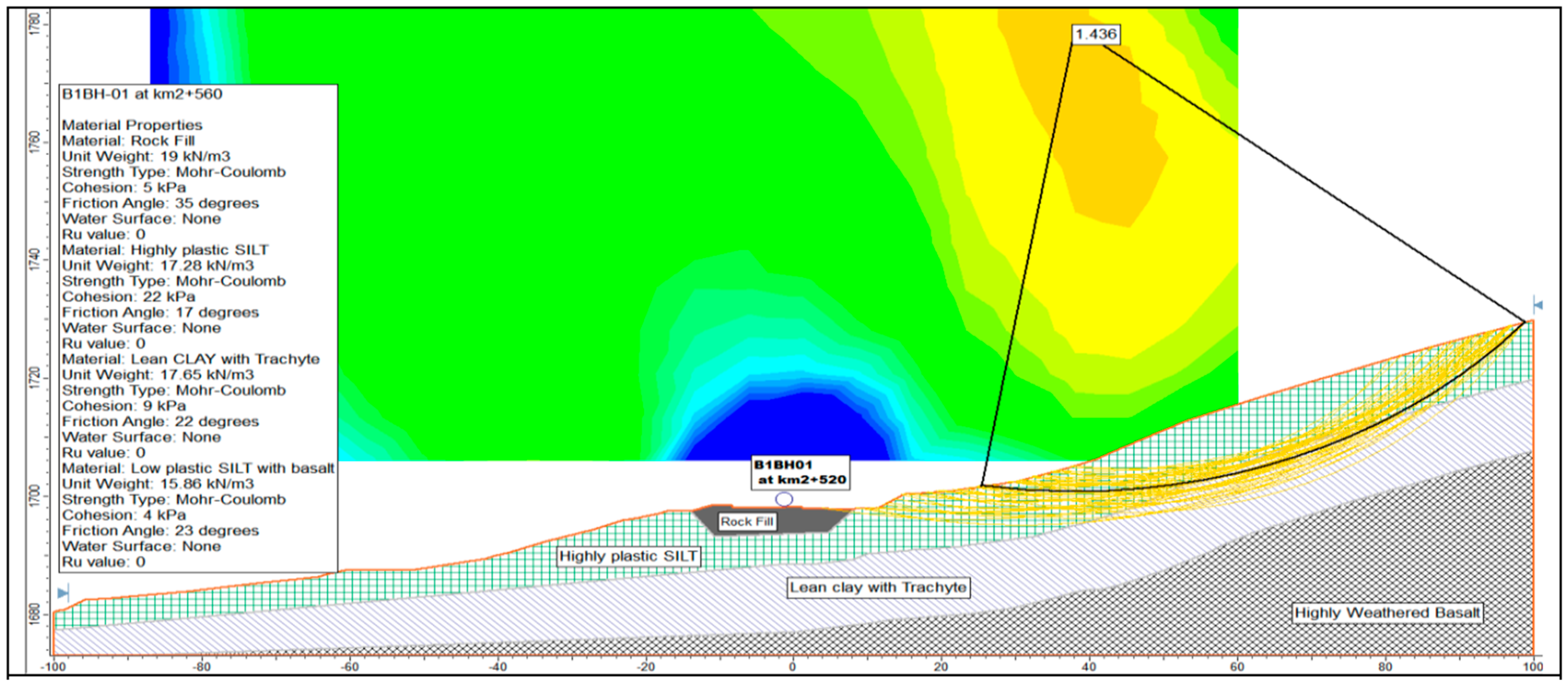
Figure 1. Sample factor of safety for Bonga 1.
Applsci 15 10613 g001
Figure 2. Correlation matrix of the dataset: (a) original and (b) synthetic data.
Applsci 15 10613 g002
Figure 3. Box plot distribution for the data set.
Applsci 15 10613 g003
Figure 4. Density plot distribution of the dataset.
Applsci 15 10613 g004
Figure 5. Distribution of safety factors in dry conditions: (a) histogram, (b) violin plot. Where Q1 is the first quartile, M is the median, and Q3 is the third quartile in the violin plot.
Applsci 15 10613 g005
Figure 6. Architecture of shallow neural networks used in this study.
Applsci 15 10613 g006
Figure 7. The flow of the proposed method.
Applsci 15 10613 g007
Figure 8. Comparison of different machine learning algorithms in the train–test split.
Applsci 15 10613 g008
Figure 9. The SVR result: (a) train–test split, (b) 5-fold cross-validation.
Applsci 15 10613 g009
Figure 10. Feature importance graph using the random forest algorithm.
Applsci 15 10613 g010
Table 1. List of landslide sections with stations and locations, along with labeling the site attribute.
Labelling of Site AttributeName of the SiteStation, kmCoordinates (UTM)
Easting Northing
1Bonga-12+500-2+650195,599.5804,260.3
2Bonga-24+300-4+420194,786.0803,588.0
3Mizan-10+960-1+220798,347.0781,820.0
4Mizan-22+420-2+620797,520.0780,693.0
5Mizan-32+800-2+860797,391.9780,450.8
6Mizan-43+040-3+140797,251.2780,265.3
7Mizan-53+400-3+550796,950.0780,590.0
8Mizan-64+230-4+320796,355.0780,752.0
9Mizan-74+720-4+780795,923.0780,821.0
10Mizan-88+740-8+810793,155.0781,716.0
11Mizan-913+400-13+520790,144.0781,233.0
Table 2. Descriptive statistics of soil parameters considered in this study.
SiteUnit WeightCohesionFriction AngleFS Dry
Count22.00000022.00000022.00000022.00000022.000000
Mean6.00000017.66454510.72727325.7727271.974273
Std3.2366940.4487205.7169917.2829340.584442
Min1.00000016.9500005.00000017.0000000.931000
25%3.25000017.5200005.00000020.2500001.545500
50%6.00000017.5650009.00000022.0000001.880500
75%8.75000018.00000015.00000035.0000002.241250
Max11.00000019.00000022.00000035.0000003.288000
Table 3. Hyperparameters of the algorithm used in this study.
Model TypeAlgorithmRoleKey HyperparametersNotes
Tree-basedXGBoostTeachern_estimators = 400, max_depth = 5, learning_rate = 0.05, subsample = 0.9, colsample_bytree = 0.9, reg_lambda = 1.0Used to pseudo-label simulated data
Tree-basedRandom ForestStudentn_estimators = 300, max_depth = None, min_samples_split = 2, min_samples_leaf = 1, random_state = 42Domain-driven simulated + original
Tree-basedDecision TreeStudentmax_depth = None, min_samples_split = 2, min_samples_leaf = 1, random_state = 42Domain-driven simulated + original
Neural NetworkShallow ANNStudent1 hidden layer, activation = ReLU, dropout = 0.2, optimizer = Adam, epochs = 200, batch_size = 8Domain-driven simulated + original
Linear ModelLinear RegressionStudentfit_intercept = True, normalize = FalseDomain-driven simulated + original
Kernel-basedSVRStudentKernel = RBF, C = 1.0, epsilon = 0.1Domain-driven simulated + original
Instance-basedKNNStudentn_neighbors = 5, weights = ‘uniform’Domain-driven simulated + original
Table 4. Results of this study using a train–test split.
MethodsR2Adjusted R2MAEMSERMSEMAPEMax Err
RF0.96630.96000.02330.00280.05310.01160.3210
DT0.93670.92480.02040.00530.07280.00930.5664
SNN 0.87660.85340.07140.01030.10160.03830.4773
LR0.67520.61400.12710.02720.16480.06870.6248
SVR0.75840.71290.09160.02020.14210.05010.6513
KNN0.74590.69800.08020.02130.14580.04240.7301
Table 5. Results of this study using 5-fold cross-validation.
MethodR2Adjusted R2MAEMSERMSEMAPEMax Err
RF0.92810.92690.02980.00770.08800.01571.2752
DT0.89160.88980.03090.01170.10810.01591.3280
SNN0.78690.78350.09720.02300.15150.05201.3354
LR0.68200.67690.13200.03430.18510.07211.4087
SVR0.75620.75230.10090.02630.16210.05551.4013
KNN0.74620.74210.09630.02730.16540.05211.4073
Table 6. A comparison with a previous study using the ML to predict slope stability.
RefLocationDataset SizeAlgorithms UsedMetrics Reported
R2MAEMSERMSEMAPE
[62]China-SVM0.86400.4208---
DT0.28860.6374---
RF0.7934----
[63]Iran327 casesGPR0.8139--0.16097.21
DT0.68300.1430-0.210512.2
[8]Multi-country (Vietnam, Malaysia, Iran, Turkey)630 casesLR0.92651.5387-2.2618 -
[64]-200 casesANN,0.6980.0650-0.0980
[65]-4586LSTM0.810----
OurEthiopia822RF0.96630.02330.00280.05310.0116
Disclaimer/Publisher’s Note: The statements, opinions and data contained in all publications are solely those of the individual author(s) and contributor(s) and not of MDPI and/or the editor(s). MDPI and/or the editor(s) disclaim responsibility for any injury to people or property resulting from any ideas, methods, instructions or products referred to in the content.