Article

A Multidisciplinary Robust Collaborative Optimization Method Under Parameter Uncertainty Based on the Double-Layer EI–Kriging Model

1
School of Mechanical Engineering, Shenyang University of Technology, Shenyang 110870, China
2
The Key Laboratory of Intelligent Manufacturing and Industrial Robots in Liaoning Province, Shenyang 110870, China
*
Author to whom correspondence should be addressed.
Appl. Sci. 2025, 15(19), 10549; https://doi.org/10.3390/app151910549
Submission received: 2 September 2025 / Revised: 23 September 2025 / Accepted: 26 September 2025 / Published: 29 September 2025
(This article belongs to the Section Applied Industrial Technologies)

Abstract

In multidisciplinary design optimization (MDO) of high-end equipment, parameter uncertainty significantly undermines performance robustness. Existing methods are limited in convergence efficiency and in controlling uncertainty propagation. To address this gap, we propose a multidisciplinary robust collaborative optimization method under parameter uncertainty (MRCO-PU). The approach augments traditional Collaborative Optimization (CO) with a collaborative optimization method based on weight distribution difference information (CO-WDDI) to accelerate cross-disciplinary convergence. It also integrates a double-layer EI–Kriging robust optimization model to enhance robustness under complex coupling and small-sample conditions. The MRCO-PU method targets single-objective, strongly coupled, multi-constraint MDO problems with high per-evaluation cost. The method was validated on a mathematical case and on a cantilever roadheader cutting-head case. In the mathematical case, the robust feasibility of the constraints increased from 0.49 to 1.00. In the engineering case, the specific energy consumption decreased by 6.3% under the premise of fully satisfying the robust feasibility of the constraints, leading to operational cost minimization under uncertainty. This work provides an effective approach to multidisciplinary robust optimization for high-end equipment.

1. Introduction

The design optimization of high-end equipment, such as ships, aircraft, and vehicles, often involves strong couplings among multiple disciplines and necessitates a systematic analysis of their interactions [1]. Multidisciplinary design optimization (MDO) is capable of addressing complex interdisciplinary couplings [2]. It seeks the global optimum while balancing conflicts among disciplines, thereby significantly shortening the design cycle [3].
Among the various MDO methods, collaborative optimization (CO) has been widely employed in engineering optimization owing to its high degree of disciplinary autonomy and favorable parallelism [4,5]. Chen et al. employed the CO method to integrate structural engineering, fluid dynamics, and energy systems, thereby improving the cruising range of the underwater helicopter and reducing the optimization cycle [6]. Zhang et al. applied the CO method in optimizing a high-speed pantograph, thereby achieving overall enhancements in motion performance, lightweight, contact force stability, and active control capability [7]. Bao et al. proposed a global–local CO method based on parameter sensitivity analysis and applied it in optimizing compressor blades, thereby enhancing both efficiency and pressure ratio [8]. Mcharek et al. integrated the CO method with knowledge management techniques and applied it in optimizing an electronic throttle body (ETB) controller, thereby improving design efficiency [9]. Shuvam et al. employed the CO method to solve the optimization of economic load dispatch (ELD) and reactive power in power grid scheduling, thereby improving voltage stability and reducing operating costs [10]. In summary, CO has been successfully applied to underwater helicopter design, high-speed pantograph optimization, compressor blade design, electronic throttle control, and power-grid dispatch. It yields measurable gains in cross-disciplinary coordination and computational efficiency for problems that are strongly coupled, constraint-dense, and computationally expensive. However, system-level consistency constraints can lead to slow convergence and significant coordination overhead in high-dimensional, multi-constraint settings. In addition, pervasive parameter uncertainty over the life cycle of high-end equipment makes robustness requirements more stringent [11].
To improve engineering design under uncertainty, uncertainty-based multidisciplinary design optimization (UMDO) has been advanced [12]. UMDO mainly comprises multidisciplinary robust design optimization (MRDO) [13] and reliability-based multidisciplinary design optimization (RBMDO) [14]. MRDO is aimed at meeting nominal performance requirements while reducing sensitivity to uncertainty and performance variability. RBMDO ensures design safety and applicability by imposing explicit reliability constraints. This study is focused on MRDO for high-end equipment. In the 1970s, Taguchi introduced robust design, which laid the foundation for robust optimization [15]. Zhao et al. proposed a unified analysis–optimization framework that simultaneously characterizes aleatory and epistemic uncertainties. They coupled the framework with transfer-matrix–based rapid dynamic analysis to enable multiobjective robust design [16]. Najlaoui et al. developed a multi-fidelity surrogate-based sequential sampling scheme. They employed a combined criterion extended upper confidence bound and probability of feasibility to jointly select sampling locations and fidelity levels, thereby improving the efficiency of robust optimization [17]. Lin et al. established a multi-objective robust optimization framework for plate heat exchangers. The framework balances performance and cost and markedly reduces sensitivity to key parameters [18]. Ma et al. proposed a multi-objective robust optimization approach that couples incremental sequential sampling with a radial basis function neural network surrogate. The approach maintains robustness while reducing computational cost [19]. Collectively, these advances demonstrate that MRDO offers practical pathways for engineering applications.
Regarding robust CO methods, Liu et al. addressed random uncertainties in design variables by employing the CO method to construct an MDO framework under uncertainty for an autonomous underwater vehicle (AUV), thereby improving the robustness of the overall scheme [20]. Zhou et al. addressed multidisciplinary couplings and parameter uncertainties in an X-by-wire chassis by integrating uncertainty analysis into bi-level integrated system collaborative optimization (BLISCO), and proposed an uncertain bi-level collaborative optimization (UBLCO) method, which effectively enhanced the reliability and robustness of the chassis under uncertainty [21]. Jin et al. developed a robust collaborative optimization framework based on Six Sigma theory and established a motor approximate efficiency model by combining it with the Kriging model, thereby effectively reducing the long-term operating cost of a plug-in hybrid electric bus under uncertainty [22]. Han et al. proposed a multifunctional collaborative optimization framework for a low-carbon data center integrated energy system (DCIES) to address the uncertainty of renewable energy, and formulated a two-stage robust optimization model based on data-driven uncertainty sets [23]. Cheng et al. proposed an efficient collaborative robust topology optimization (CRTO) method for structural optimization of functionally graded materials under hybrid probabilistic and non-probabilistic uncertainty, thereby significantly reducing the computational burden [24]. Robust CO has been validated in applications including AUVs, X-by-wire chassis, plug-in hybrid electric buses, data-center integrated energy systems, and functionally graded materials. It has been shown to reduce variability under uncertainty and enhance robustness. However, in strongly coupled MDO settings for high-end equipment, bidirectional uncertainty propagation across disciplines and levels can significantly increase the problem size and computational costs of global robust optimization. More efficient cross-level coordination and robust optimization strategies are therefore needed.
To address the challenges of cross-level uncertainty transmission and high computational cost, surrogate models have become an essential tool for multidisciplinary robust optimization. In particular, the Kriging model offers high computational efficiency and approximation accuracy, and is especially suitable for small-sample, highly nonlinear engineering optimization problems [25,26].
To address the effects of parameter uncertainty on the design optimization of high-end equipment, a multidisciplinary robust design optimization method that integrates high-fidelity modeling with efficient computation is proposed. The method targets multidisciplinary robust optimization problems for high-end equipment, which are typically characterized by multiple constraints and strong coupling. The main contributions of this work are as follows:
(1) A collaborative optimization method based on weight distribution difference information (CO-WDDI) is proposed. By exploiting the differences among disciplines and the deviations between disciplinary design points and system-level expectations, the relaxation factors are reconstructed, thereby significantly improving the convergence speed and computational efficiency of the CO method.
(2) A double-layer EI–Kriging robust optimization model (DL-EI–Kriging) is introduced. The inner layer suppresses discipline-level local uncertainty fluctuations, while the outer layer prevents the bidirectional propagation of uncertainty between the system and discipline levels, thereby achieving coordinated control of uncertainties across both levels.
(3) A multidisciplinary robust collaborative optimization method under parameter uncertainty (MRCO-PU) is proposed, integrating CO-WDDI and DL-EI–Kriging into a unified robust collaborative optimization framework. The method is validated on a mathematical case and on an engineering case of a cantilever roadheader cutting head. Performance is assessed using metrics including objective value, iteration count, computation time, and robust feasibility. Results indicate that MRCO-PU offers significant advantages in global robustness and engineering applicability.
The remainder of this paper is organized as follows: Section 2 introduces CO-WDDI and its solution process. Section 3 describes the principles of the Kriging model and the EI criterion, and then presents the DL-EI–Kriging robust optimization model. Section 4 details the MRCO-PU method, including robustness analysis and solution steps. Section 5 demonstrates the effectiveness and engineering applicability of the proposed method through a mathematical case and an engineering example. Finally, Section 6 presents the summary and conclusions.

2. Collaborative Optimization Method Based on Weight Distribution Difference Information

2.1. Traditional Collaborative Optimization (CO)

The CO method is characterized by a high degree of disciplinary autonomy, which effectively reduces the complexity of the solution process and improves computational efficiency. It is well-suited for multi-parameter and highly nonlinear MDO problems [6,27]. The basic idea is to decompose the MDO problem into system-level and discipline-level [28]. First, the system level transfers the system expectations to each discipline level. Each discipline independently solves its subproblem within its own design variables and local constraints, obtaining the disciplinary optimum that approaches the system expectations. Subsequently, each discipline returns its optimal solution to the system level. The system level accordingly constructs consistency equality constraints, coordinates the disciplines, and minimizes the global objective function. Through multiple iterations, the global optimal solution is eventually achieved. The structure of CO is illustrated in Figure 1.
The system-level optimization model in the CO method is formulated as
min F z s . t . J i * z = j = 1 m X i j * Z j 2 = 0 , i = 1 , 2 , n h z = 0 , g z 0
where F z denotes the system-level objective function; X i j * is the j t h system-level design variable obtained from the optimization of the i t h discipline; m represents the number of design variables shared by the system and discipline levels; Z j is the j t h system-level design variable; J i * z specifies the consistency constraints linking the system and discipline levels; h z denotes the system-level equality constraints; and g z denotes the system-level inequality constraints.
The discipline-level optimization model is formulated as follows:
min J i X i J i X i = i = 1 m X i j * Z j 2 , i = 1 , 2 , , n s . t . g X i j X i l 0 , j = 1 , 2 , , m
where J i X i is the objective function of the J i * discipline; X i j * is the j t h design variable of the i t h discipline; X i l denotes the local design variable of the i t h discipline; Z j represents the expected value of the j t h system-level design variable transferred to the i t h discipline; and g X i j X i l specifies the constraint function at the discipline level.

2.2. Collaborative Optimization Method Based on Weight Distribution Difference Information (CO-WDDI)

The traditional CO method faces challenges in enforcing system-level consistency equality constraints in engineering applications and is often limited by slow convergence and low computational efficiency. To address these issues, this section introduces the Collaborative Optimization Method Based on Weight Distribution Difference Information (CO-WDDI) [29]. The method employs a stepwise relaxation strategy, reconstructing the relaxation factors by assigning weights based on both inter-disciplinary differences and the deviations of discipline design points from the system expectation. The relaxation factors are dynamically updated and progressively reduced during the iterations, thereby enhancing global convergence and improving computational efficiency.

2.2.1. Disciplinary Differences

Following k iterations of CO-WDDI, the optimal design solution for the i t h discipline is denoted as X i , and the norm is defined as
J i j k = X i X j
J k = max J i j k , i , j = 1 , 2 , , n , i j
Here, J i j k denotes the discrepancy between the discipline optimization results after the k - th iteration. For an MDO problem involving n disciplines, a total of n n 1 / 2 such norms exist. J k represents the maximum discrepancy among the optimal design points of the disciplines.

2.2.2. Discrepancy Between the System-Level Design Point and the Mean of Discipline-Level Design Points

Following k iterations of CO-WDDI, the system-level optimal design point is denoted as Z , with the norm defined as:
U k = Z X ¯
X ¯ = i = 1 n X i 1 * n , i = 1 n X i 2 * n , , i = 1 n X i j * n
In this equation, U k denotes the difference between the mean optimization result of all discipline levels at the k - th iteration and the system-level optimization result obtained at the same k - th iteration. Here, n is the number of discipline levels, and X ¯ denotes the mean of the optimal solutions across n discipline levels after the k - th iteration.

2.2.3. Weighting Coefficients

At the k - th iteration of CO-WDDI, J k and U k are obtained from Equations (3) and (5), and the weighting coefficients λ 1 and λ 2 are defined as
λ 1 = U k U k + J k λ 2 = J k U k + J k
where λ 1 and λ 2 are the coefficients of U k and J k . When the system-level problem is difficult to solve, λ 1 reduces the weight of inter-disciplinary discrepancies, thereby relaxing the overlapping region of the disciplinary optimal solutions, enlarging the feasible domain at the system level, and alleviating the difficulty of solving. Conversely, when the system-level problem is relatively easy to solve, λ 2 increases the weight of inter-disciplinary discrepancies, driving the disciplinary design points to cluster together and synchronously converge toward the system-level optimal solution.

2.2.4. Reformulation of the Relaxation Factor

At the k - th iteration of CO-WDDI, the relaxation factor ε in the system-level consistency constraints is defined as:
ε = λ 1 U k + λ 2 J k
The reconstructed relaxation factor allows the system-level optimization to be divided into two cases: (1) When U k > J k , it indicates that the discrepancies between the disciplines and the system are relatively large. In this case, λ 1 guides the system-level optimization to primarily reduce the difference between the discipline design points and the system-level expected value, and U k decreases progressively during the iterations. (2) When U k < J k , it indicates that the discrepancies among disciplines are relatively large. In this case, λ 2 drives the system-level optimization to primarily reduce the differences among disciplines, while J k decreases progressively during the iterations. With the adjustment of the relaxation factor, the discipline-level and system-level design points approach each other and eventually converge. The reconstructed relaxation factor reduces both the discrepancies among discipline-level design points and those between discipline and system levels, thus enhancing convergence rate and computational efficiency.

2.2.5. Procedure of the CO-WDDI Method

Step 1: The system-level provides the initial design point Z ;
Step 2: Each discipline independently optimizes and provides its design point X ;
Step 3: Compute the inter-disciplinary difference J k using Equation (4), and then compute the mean of the disciplinary design points X ¯ using Equation (6).
Step 4: Using X ¯ and Z , compute the deviation U k between discipline-level solutions and the system according to Equation (5).
Step 5: According to Equation (8), reconstruct the relaxation factor ε at the system level. After obtaining the new system-level design point, return to Step 2 until the convergence condition ε 1 × e 4 is met.
The improvements of CO-WDDI in terms of convergence speed and computational efficiency will be validated through the mathematical case presented in Section 5.

3. Double-Layer Nested EI–Kriging Robust Optimization Model

3.1. EI–Kriging Model

3.1.1. Kriging Model

The Kriging model comprises a regression term and a stochastic process term; its mathematical formulation is given as follows:
f x = i = 1 p q i x β i + Z x
where f x represents the approximate objective function, x denotes the vector of design variables, q i x is the regression basis function, and β i is its coefficient; Z x is a Gaussian stochastic process with zero mean and variance σ z 2 , and its covariance matrix is expressed as follows:
C o v Z x i , Z x j = σ z 2 R θ , x i , x j
where R θ , x i , x j represents the correlation function of two sample points x i and x j , and the Gaussian correlation function is defined as
R x i , x j = exp k = 1 d θ k x k i x k j 2
where θ k is the correlation parameter to be determined, used to characterize the correlation between sampling points. The predicted mean f ^ x of the Kriging model at an unknown point x is expressed as
f ^ x = q x T β ^ + r T x R 1 F Q β ^
where β ^ denotes the estimated regression coefficients, F represents the responses at the sample points, Q is the m × p matrix formed by the regression model of the m sample points, and r T x denotes the correlation function between the sample points and the prediction point x.
The prediction variance of the response is given by
s 2 x = σ ^ 2 1 r T x R 1 r x + u x T Q T R 1 Q 1 u x u x = q x Q T R 1 r x
The estimates of parameters β ^ and σ ^ 2 are obtained, respectively, through the following formulas:
β ^ = Q T R 1 Q 1 Q T R 1 F
σ ^ 2 = 1 m F Q β ^ T R 1 F Q β ^
The correlation parameter θ is estimated by minimizing the negative log-likelihood, that is
min θ > 0 m ln σ ^ 2 + ln R θ
The correlation parameter θ is estimated by minimizing the negative log-likelihood, as given in Equation (16), and the resulting Kriging model corresponds to the minimum-error model.

3.1.2. Expected Improvement Criterion (EI)

To enhance the accuracy of both the inner- and outer-layer Kriging models, the EI criterion is employed in both layers to incorporate additional sampling points. The EI criterion determines the next sampling point based on the predicted mean and the associated uncertainty information provided by the surrogate model. Denote the minimum response value of the currently observed samples as f min . The objective function at an unknown point x is regarded as a random variable Y x . Accordingly, the improvement at the unknown point x is defined as follows:
I x = max f min Y x , 0
The expected improvement is defined as
E I x = E I x = f min f ^ x Φ f min f ^ x s x + s ^ x ϕ f min f ^ x s x
where Φ and ϕ denote the cumulative distribution function and the probability density function of the standard normal distribution, respectively. f ^ x denotes the predicted mean, as s x denotes the predicted standard deviation s x = s 2 x . When s x = 0 , E I x is set to zero.

3.1.3. Model Construction Procedure

Step 1: Latin Hypercube Sampling (LHS) is employed within the design space to generate an initial sample set.
Step 2: A Kriging model of the objective function is constructed based on the initial sample set. Particle Swarm Optimization (PSO) is then applied to determine the current minimum of the model, and the Expected Improvement (EI) criterion is evaluated in its neighborhood to obtain the point with the maximum EI value.
Step 3: The maximum EI point is added to the sample set as a new sample.
Step 4: The Kriging model is reconstructed using the updated sample set to enhance the accuracy of the model.
The accuracy validation of the EI–Kriging model is presented in Section 5.1.

3.2. Double-Layered Nested EI–Kriging Robust Optimization Model (DL-EI–Kriging)

To mitigate the bidirectional propagation of uncertainty within the discipline level and between the system and discipline levels, this study proposes the DL-EI–Kriging Robust Optimization Model. In this framework, the inner layer constructs EI–Kriging models for the discipline-level constraint functions to mitigate local variations, while the outer layer constructs EI–Kriging models for the system-level objective and constraint functions to suppress inter-level propagation. Then, CO-WDDI is employed for system-level coordination to ensure the consistency of the global robust solution and to enhance its convergence efficiency.
The CO-WDDI method is employed to decouple the multidisciplinary problems, and the resulting model takes the form of a multilevel optimization framework. The corresponding system-level optimization model is formulated as
min F ^ Z = F ^ Z , Z U s . t . J i * Z , Z U ε , i = 1 , 2 , , n
Here, F ^ denotes the surrogate model of the objective function, represents the deterministic design variables, and Z U represents the uncertain design variables. The regression function of the surrogate model is expressed as Equation (20):
F ^ Z , Z U = q Z , Z U T β ^ + r T Z , Z U R 1 F Q β ^ J ^ i ( Z , Z U ) = q Z , Z U T δ ^ + r T Z , Z U R 1 J B δ ^
In the equation, β ^ and δ ^ denote the regression coefficient matrices obtained by the best linear unbiased estimator. F denotes the response of the system-level objective function, and J denotes that of the constraint functions. Q and B are polynomial matrices. After constructing the system-level Kriging model, new samples are selected based on the EI criterion to improve the surrogate accuracy. Thus, the construction of the system-level optimization model is completed.
The discipline-level optimization model can be formulated as:
min J i X i = J i X , X U s . t . h ^ i X , X U = 0 g ^ i X , X U 0
Here, X denotes the deterministic design variables of discipline i , X U denotes the uncertain design variables of discipline i , and h ^ i along with g ^ i denote the Kriging-based approximations of the equality and inequality constraint functions of discipline i , respectively. The detailed fitting procedure is given in Equation (22).
h ^ i X , X U = q X , X U T λ ^ + r T X , X U R 1 H D λ ^ g ^ i X , X U = q X , X U T ω ^ + r T X , X U R 1 G P ω ^
In the equation, λ ^ and ω ^ denote the regression parameter matrices obtained by the Best Linear Unbiased Estimator, H and G denote the response functions. D and P denote the polynomial matrices. The discipline-level optimization model is constructed in the same manner as the system-level model.

4. Multidisciplinary Robust Collaborative Optimization Method Under Parameter Uncertainty

4.1. Robustness Analysis

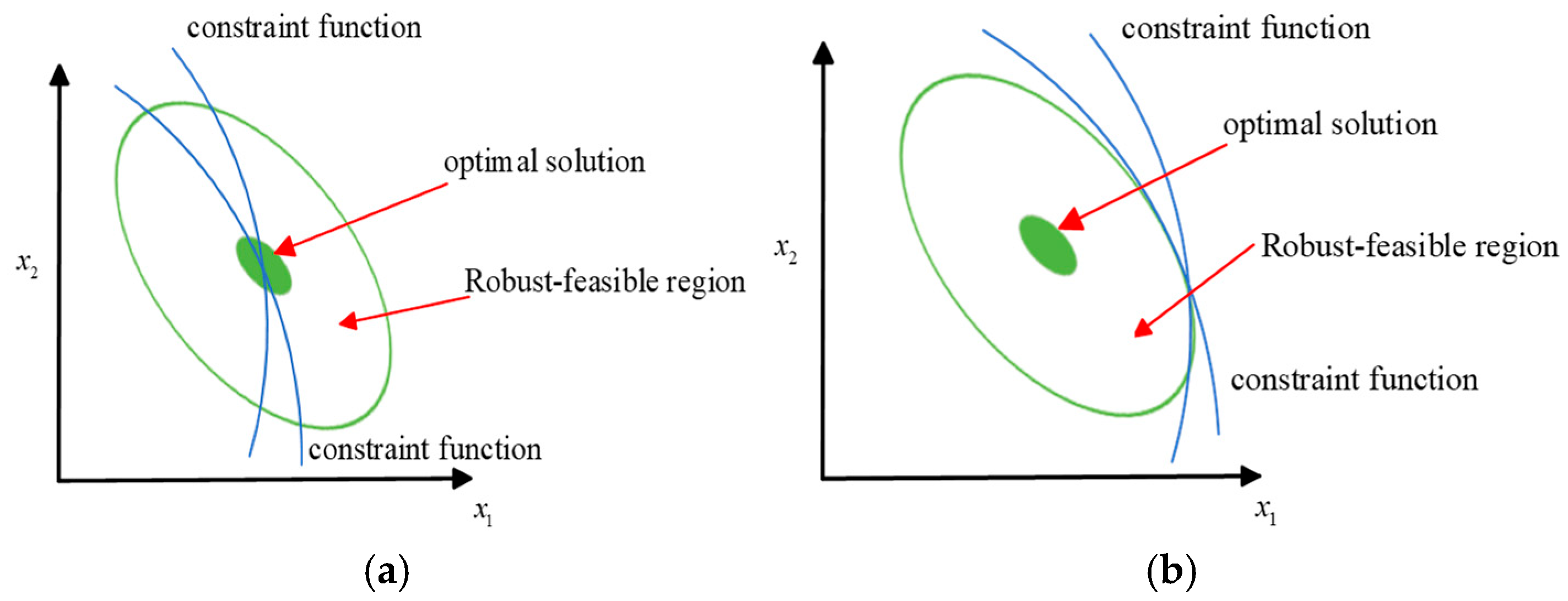
The optimal solution of deterministic optimization is usually located near the constraint boundary. When the design variables are perturbed by uncertainty, the solution may cross the boundary and become infeasible, as illustrated in Figure 2. Hence, robust optimization is employed to mitigate the risk of constraint infeasibility. In MDO, uncertainty analysis is typically based on probability distributions [30]. However, it is often difficult to obtain complete probabilistic information in engineering practice [31]. To address this issue, the interval method is employed in this study to quantify uncertainty. Unlike conventional probability-based modeling, the interval method defines the uncertainty set using only the upper and lower bounds of parameters, which offers simplicity and better aligns with engineering practice [32,33].
Robustness analysis concerns the robustness of the objective function and the robust feasibility of the constraint functions. The robustness of the objective function means that, when subjected to uncertainty perturbations, it varies only within an acceptable range. The robust feasibility of the constraints means that, under uncertainty, the constraint functions continuously satisfy feasibility requirements without failure [34]. The robust feasibility of constraints more effectively reflects the capacity of equipment to resist uncertainties and is therefore more critical in engineering practice. To simplify the computation, this study first ensures the robust feasibility of constraints and then minimizes the objective function within the feasible domain.

4.2. Procedure of the MRCO-PU Method

Before the procedure is described, the systematic rationale for method selection and the integrative mechanism are outlined. MRDO problems are characterized by strong nonlinearity, expensive evaluations, and interval uncertainty. Accordingly, candidates were screened across optimizers, surrogate models, active sampling, and multidisciplinary coordination strategies. Screening criteria included data efficiency, global search capability, uncertainty representation, interpretability, convergence stability, and engineering practicality. CO-WDDI was ultimately adopted. It preserves disciplinary autonomy in a collaborative optimization setting and stabilizes the convergence of the consistency constraints through adaptive reconstruction of the relaxation factor. Kriging served as the surrogate model, providing reliable approximations and practical implementation in small-sample, coupled multidisciplinary settings, thereby furnishing a reliable basis for robust constraint determination. EI served as the active sampling criterion. Under small-sample, expensive-evaluation conditions, EI balanced exploration and exploitation, and sequential infill was performed to improve the accuracy and stability of the Kriging model. PSO was employed as the solver owing to its mature implementations, clear parameterization, and easy integration with the present workflow. Initial samples were generated using LHS to ensure adequate sampling across each dimensional interval and to enhance coverage of the design space.
LHS, CO-WDDI, EI–Kriging, and PSO were integrated because of their complementarity in computational resource use and multidisciplinary coordination. LHS provides a balanced initial sample set. EI–Kriging incrementally refines the model through sequential infill. In CO-WDDI, adaptive relaxation driven by difference weights is employed to accelerate and stabilize the coordination of the consistency constraints and to reduce coordination overhead. Finally, the optimization was performed using PSO. Consequently, under a limited evaluation budget, robustness, computational efficiency, and convergence stability were maintained.
The methods in this study can be classified as follows: CO-WDDI is a multidisciplinary optimization method, EI–Kriging is a surrogate model–based robust optimization method, and MRCO-PU is an integrated framework for multidisciplinary robust optimization, constructed by integrating the two.
Building on the above method-selection rationale and integrative mechanism, the MRCO-PU framework was constructed with CO-WDDI and DL-EI–Kriging. The procedure is as follows:
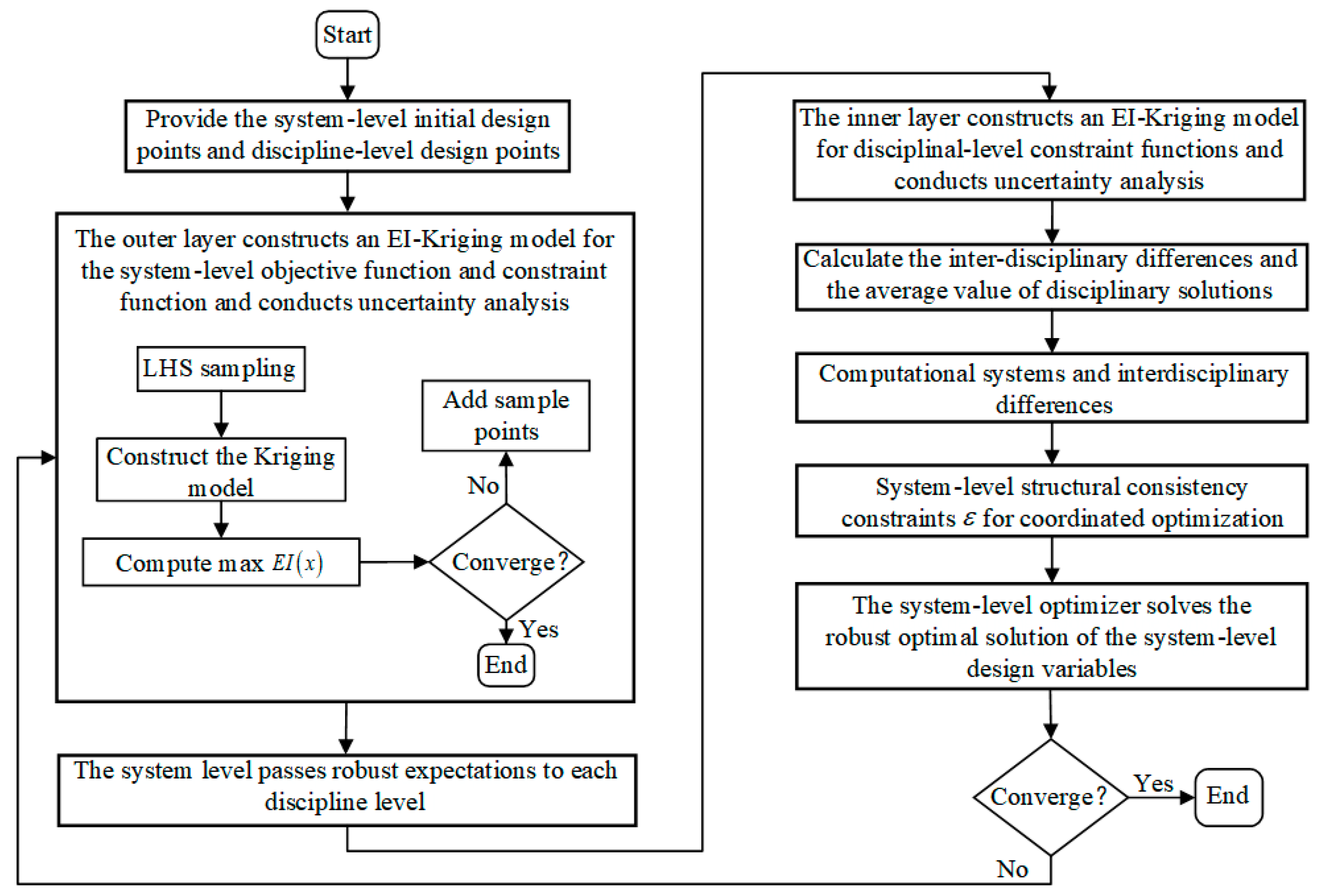
The MRCO-PU method is developed using the CO-WDDI approach and the DL-EI–Kriging model. The procedure is outlined as follows:
Step 1: The system-level optimizer gives the initial system design point, while each discipline-level optimizer gives its respective initial design point.
Step 2: In the outer layer, EI–Kriging models are constructed for the system-level objective and constraint functions, and uncertainty analysis is performed to derive the robust expected value at the system level.
Step 3: The system-level transmits this robust expected value to each discipline level.
Step 4: In the inner layer, EI–Kriging models are constructed for the discipline-level constraint functions, followed by uncertainty analysis to obtain the robust optimal solutions for each discipline.
Step 5: Based on the robust optimal solutions of each discipline, calculate the inter-disciplinary discrepancy information J k and the mean of the disciplinary solutions X ¯ .
Step 6: Use X ¯ and the system-level robust expected value to calculate the system–discipline discrepancy information U k .
Step 7: At the system level, formulate the consistency constraint ε and perform coordination optimization to obtain a new system-level robust solution. If ε 1 × e 4 , the iteration terminates; otherwise, return to Step 2 to continue the iteration.
The process of the MRCO-PU method is illustrated in Figure 3.

5. Experimental Validation

5.1. EI–Kriging Model Verification

In this section, a two-dimensional test function is employed to validate the EI–Kriging model. The test problem is defined as
min f x 1 , x 2 = 0.01 x 1 x 2 2 2 + 1 x 2 + 2 4 x 1 2 + 7 sin 0.5 x 2 sin 0.5 x 1 x 2 s . t .2 x 1 7 , 0 x 2 5
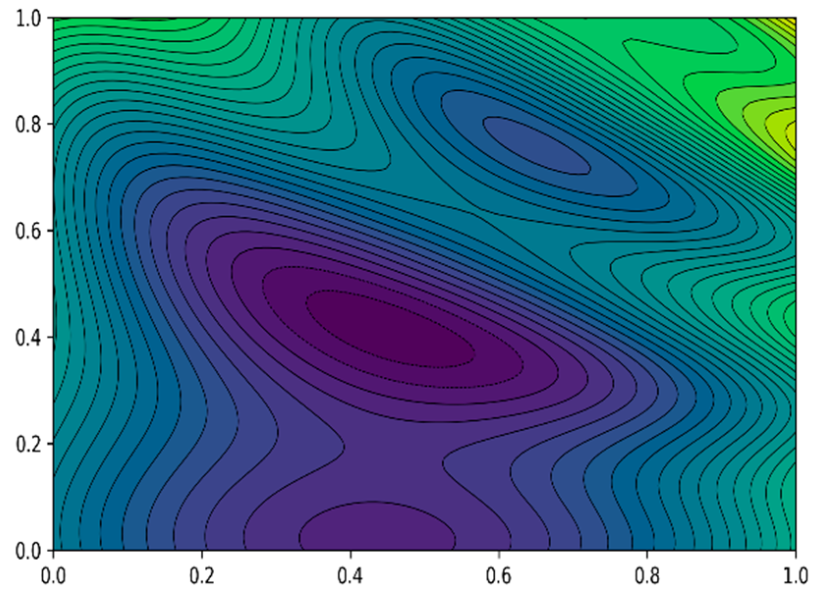
In the equation, f represents the true objective function, with x 1 and x 2 as the design variables, normalized accordingly. Figure 4 presents the true contour map. The function exhibits highly nonlinear characteristics, making it suitable for evaluating the sampling efficiency and prediction accuracy of the EI–Kriging model.
LHS is adopted to generate 20, 30, and 40 sample points, respectively. A Kriging model is then trained using these samples to approximate the test function, and the corresponding contour plots are shown in Figure 5. As the number of sample points increases, the Kriging model becomes more consistent with the true model. However, a significant deviation still remains. This demonstrates that relying solely on the initial samples is insufficient to achieve the required accuracy.
Subsequently, the EI criterion is adopted to add new sample points to the Kriging model, and the positions of the points added by the EI criterion are marked. The number of EI-added points is set to 10. As shown in Figure 6, the EI–Kriging model approaches the true model more closely, and the newly added samples are primarily distributed near the predicted optimum.
The comparison results indicate that the EI–Kriging model achieves a higher goodness of fit for this test problem and is closer to the true response. Moreover, the sample points selected by the EI criterion are primarily concentrated near the predicted optimum, with their distribution largely consistent with the optimal region.

5.2. Mathematical Case Validation

The validation in Section 5.1 indicates that the EI–Kriging model has already acquired the fitting accuracy required for robust optimization. To further evaluate the proposed MRCO-PU method, a classical mathematical case is employed in this section for validation. This case involves three design variables, two coupled state variables, and two inequality constraints. Since equality constraints are difficult to satisfy strictly in engineering practice, the original equality constraints are relaxed to inequality constraints with a tolerance. According to the decomposition strategy of MRCO-PU, the case is decomposed into one system-level problem and two discipline-level subproblems. Its mathematical model is formulated as follows:
min f X , Y = x 2 2 + x 3 + y 1 + e y 2 s . t . g 1 = 1 y 1 / 8 0 g 2 = y 2 / 10 1 0 y 1 = x 1 2 + x 2 + x 3 0.2 y 2 y 2 = y 1 + x 1 + x 3 10 x 1 10 ; 0 x 2 10 ; 0 x 3 10
The system-level mathematical model is formulated as follows:
min f X , Y s . t . J 1 = z 1 x 1 1 2 + z 2 x 2 1 2 + z 3 x 3 1 2 + y 1 y 1 1 2 + y 2 y 2 1 2 ε 2 s . t . J 2 = z 1 x 1 2 2 + z 3 x 3 2 2 + y 1 y 1 2 2 + y 2 y 2 2 2 ε 2
The mathematical model of Discipline 1 is formulated as follows:
min J 1 * = z 1 x 1 1 2 + z 2 x 2 1 2 + z 3 x 3 1 2 + y 1 y 1 1 2 + y 2 y 2 1 2 s . t . 10 x 1 10 ; 0 x 2 10 ; 0 x 3 10
The mathematical model of Discipline 2 is formulated as follows:
min J 2 * = z 1 x 1 2 2 + z 3 x 3 2 2 + y 1 y 1 1 2 + y 2 y 2 1 2 s . t . 10 x 1 10 ; 0 x 3 10
To assess the convergence efficiency of CO-WDDI, a comparative evaluation against Analytical target cascading (ATC) [35] and traditional CO was performed across three distinct initial points. As shown in Table 1, CO-WDDI converged in only 16, 20, and 34 iterations, with computation times of 4, 3, and 5 s, respectively, and achieved an objective value of 8.00 in all three cases. By contrast, traditional CO required 24, 89, and 40 iterations, with computation times of 4, 11, and 8 s, achieving objective values of 7.52, 7.46, and 8.96, respectively. ATC required 35, 102, and 57 iterations, with computation times of 12, 25, and 14 s, achieving objective values of 7.36, 8.68, and 6.32, respectively. Overall, under identical initial settings and evaluation budgets, convergence was achieved by CO-WDDI with fewer iterations and shorter computation times, consistently attaining an objective value of 8.00. By contrast, traditional CO and ATC incurred greater convergence overhead and yielded objective values deviating from 8.00, indicating that CO-WDDI exhibits superior convergence efficiency and solution stability.
After establishing the convergence-efficiency advantage of CO-WDDI, it was used as the deterministic optimization method. For comparison, the UBLCO robust optimization method [21] and the proposed MRCO-PU were considered. The objective was to evaluate differences in objective value and robust feasibility of constraints under parameter uncertainty. In the case study, x 1 , x 2 , x 3 a were modeled with interval uncertainty within Δ x = ± 0.1 . Using the first set of initial points as an example, we compared three strategies: deterministic optimization, UBLCO, and MRCO-PU.
To examine the robust feasibility of the constraint functions g 1 and g 2 under uncertainty, the LHS method was first used to sample 400 points for each function to construct the Kriging model. Subsequently, 100 additional sample points were incorporated into the model in accordance with the EI criterion. This step was performed to improve the model accuracy. The measure of robust feasibility is defined as the ratio of the number of samples satisfying g 0 to the total number of samples. Table 2 presents the results of robust feasibility verification for three strategies. Deterministic optimization yields approximately 0.49, indicating inadequate robustness. UBLCO achieved robust-feasibility rates of 0.9211 for g 1 and 0.9038 for g 2 . These values exceeded those of the deterministic method. MRCO-PU achieved 1.0 for both constraints, fully satisfying the robust-feasibility criterion.
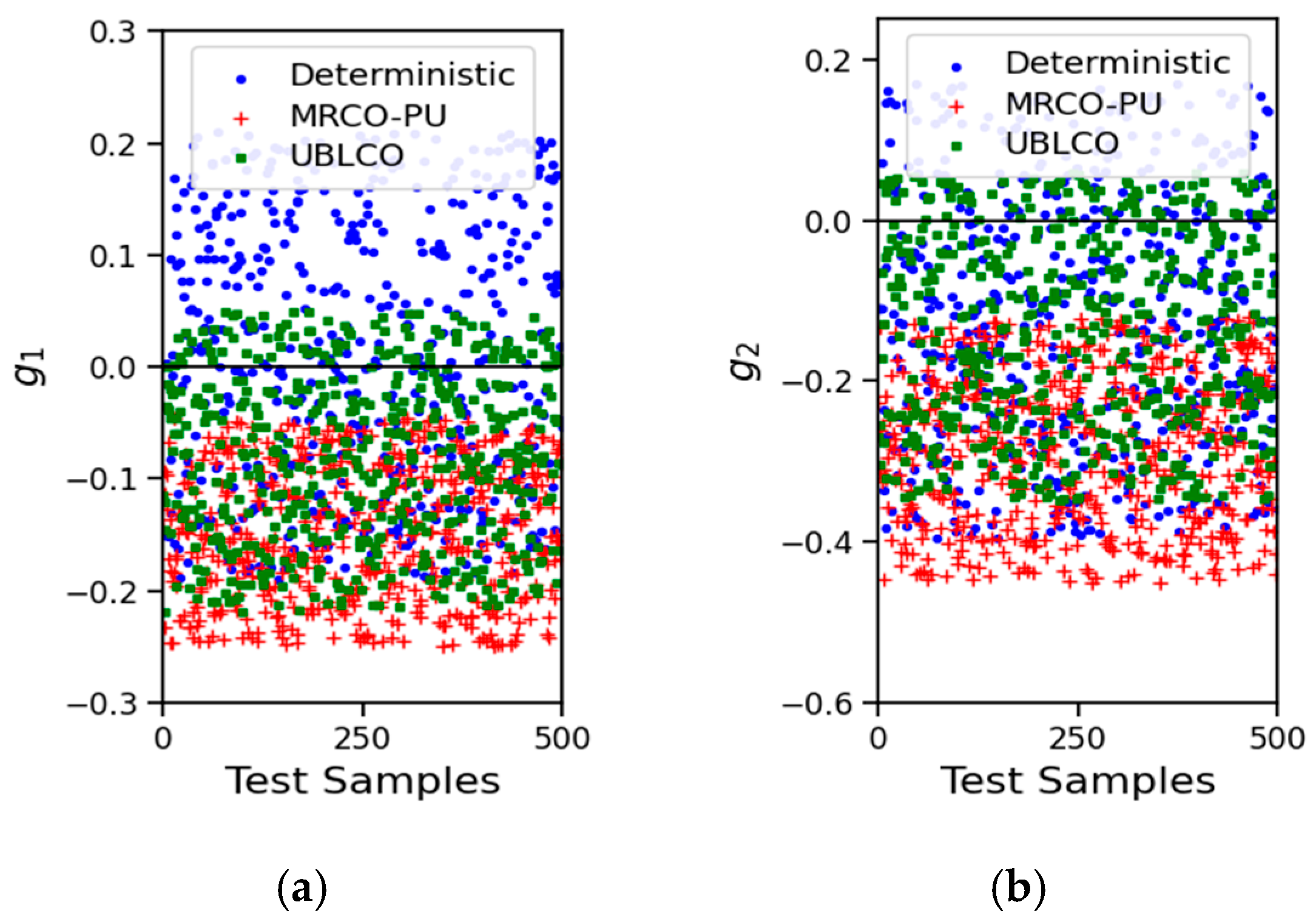
Figure 7 shows that, under uncertainty perturbations, the constraint functions of deterministic optimization exceed the feasibility range of g 0 multiple times. Compared with deterministic optimization, UBLCO shows a clear improvement; however, a few constraint-failure instances still occur. For MRCO-PU, no constraint failures were observed within the test samples. These results demonstrate that MRCO-PU suppresses uncertainty propagation and consistently maintains the robust feasibility of the constraints, providing a sound basis for subsequent comparisons of the objective functions.
Accordingly, Table 3 presents the optimal solutions of the first group of initial points under the three strategies. The objective function value of deterministic optimization is 8.00. Under uncertainty, the objective values for UBLCO and MRCO-PU were 8.17 and 8.08, respectively. This indicates that the MRCO-PU method increases the objective function value by only 1%, and the increase remains within the acceptable range.

5.3. Engineering Case Validation

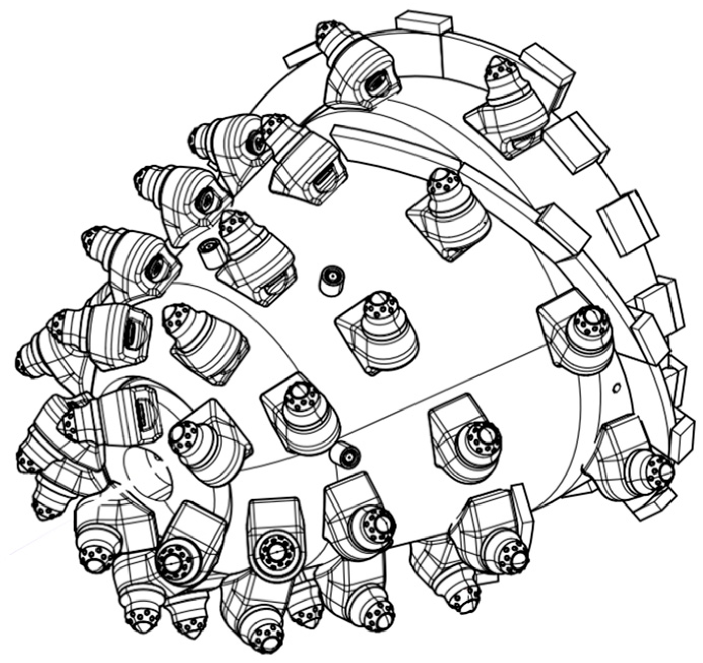
The cutting head is the core working component of a cantilever roadheader, typically consisting of cutting picks, pick holders, a base body, and connecting mechanisms. By means of the cutting picks, it impacts, cuts, and compresses the coal and rock to achieve their fragmentation and removal. The performance of the cutting head plays a decisive role in determining the operational efficiency and overall performance of the roadheader. Based on this, the cutting head optimization problem is introduced in the engineering case. This not only demonstrates the engineering applicability of the proposed method but is also of significant practical importance. However, in complex and dynamic engineering environments, the cutting head is inevitably affected by parameter uncertainty arising from manufacturing process variation, material-property fluctuations, and operating-condition changes. The above uncertainties not only increase performance fluctuation risks but also reduce the robustness of the design solution. Hence, robust optimization is required to enhance the robustness and adaptability of the cutting head under parameter uncertainty. Figure 8 shows the assembly of the cutting head.
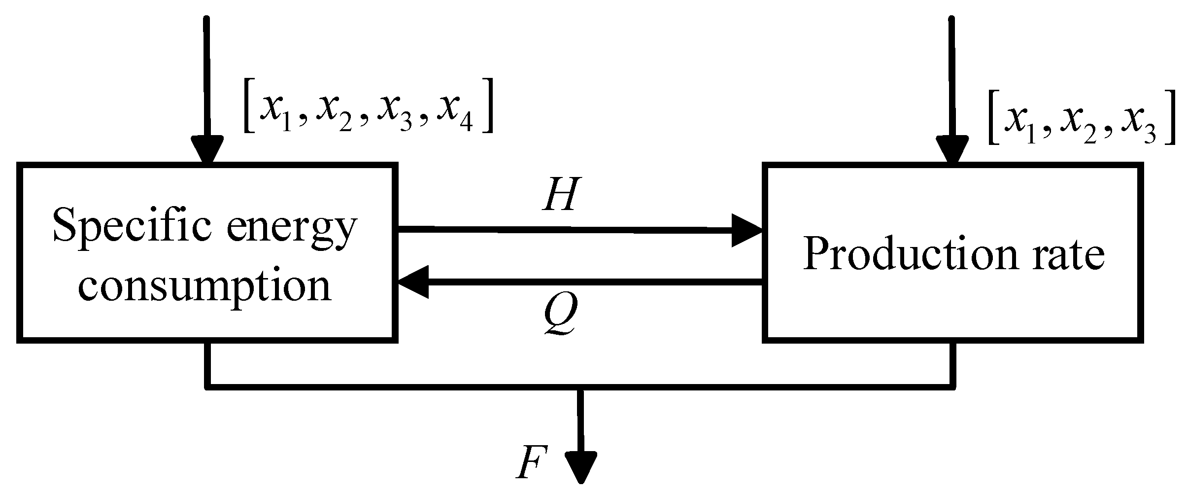
After validating the effectiveness and robustness of the MRCO-PU method with a mathematical case, the cutting head of the EBZ180 cantilever roadheader is chosen as the engineering example in this section. This equipment is primarily used for coal and rock excavation with hardness f ≤ 8. Based on the core indicators of cutting head performance evaluation, specific energy consumption and production rate are chosen as the basis for disciplinary decomposition. A multidisciplinary robust collaborative optimization model is then constructed to assess the applicability and feasibility of the MRCO-PU method under parameter uncertainty, and to minimize the operating cost. The disciplinary decomposition is illustrated in Figure 9.
The cutting head optimization problem involves four design variables and seven inequality constraints. Among them, x 1 and x 3 are subject to uncertainty. Their uncertainty interval is defined as Δ x = ± 10 , which corresponds to approximately 1% of the nominal dimension. The specified parameter interval covers manufacturing process variation and minor variations arising from material properties and environmental changes. This specification represents uncertainty in engineering practice while avoiding risk underestimation and undue expansion of the design space. As a result, the feasibility and robustness of the optimization outcomes are maintained. The remaining variables are deterministic design variables. The design variables and their ranges are provided in Table 4.
The mathematical model for the cutting-head optimization problem is formulated as follows:
min F x = H w x + Q s 1 x s . t . g 1 = 1000 x 2 x 4 0.9 L p 0 g 2 = t 2.5 1000 x 2 x 4 0 g 3 = 1.5 1000 x 2 x 4 t 0 g 4 = 30 arccos 1 2 h x 3 0 g 5 = arccos 1 2 h x 3 60 0 g 6 = 1.5 M ¯ c x 4 9550 P n 0 g 7 = Q 0 60 λ 0 x 1 x 2 x 3 0 800 x 1 1000 , 0.8 x 2 1.5 600 x 3 1000 , 20 x 4 50
In the equation, H w x = 2 π n M ¯ c v L D denotes the specific cutting energy consumption MJ / m 3 . Q S X = 60 λ 0 L D v denotes the production rate m 3 / h , L p is the protrusion length of the cutting pick mm , taken as 82. t is the spacing between cutting picks mm , taken as 45.68. h is the cutting thickness of the pick at any position m m , taken as 26.09. M ¯ c denotes the average load torque N m , taken as 134,045. λ 0 is the loosening coefficient of coal and rock, taken as 1.5. Q 0 is the production rate before optimization m 3 / h , taken as 62.22.
The system-level model is given as
min F x s . t . J 1 = z 1 x 1 1 2 + z 2 x 2 1 2 + z 3 x 3 1 2 + z 4 x 4 1 2 ε 2 J 2 = z 1 x 1 2 2 + z 2 x 2 2 2 + z 3 x 3 2 2 ε 2
The mathematical model of the specific energy consumption is given as
min J 1 = z 1 x 1 1 2 + z 2 x 2 1 2 + z 3 x 3 1 2 + z 4 x 4 1 2 s . t . g i 0 , i = 1 , 2 , 3 , 4 , 5 , 6 , 7
The mathematical model of the production rate is given as
J 2 = z 1 x 1 2 2 + z 2 x 2 2 2 + z 3 x 3 2 2 s . t . g i 0 , i = 1 , 2 , 3 , 4 , 5 , 6
To assess the convergence efficiency of CO-WDDI, Table 5 presents a comparison of ATC, traditional CO, and CO-WDDI on the Cutting Head case under the same initial design. Convergence with ATC required 46 iterations and 15 s, yielding an objective value of 90.55. Among the three methods, ATC exhibited the largest iteration count and runtime and yielded the highest objective value. Traditional CO achieved convergence in 34 iterations and 14 s with an objective of 88.05, showing improvements over ATC. CO-WDDI achieved convergence in only 16 iterations and 4 s, with an objective of 87.02. Consequently, relative to ATC and traditional CO, CO-WDDI reduced the iteration count by 30 and 18 steps and shortened runtime by 11 and 10 s, respectively, while attaining a lower objective value (the objective is minimized in this case), indicating superior convergence efficiency and solution stability.
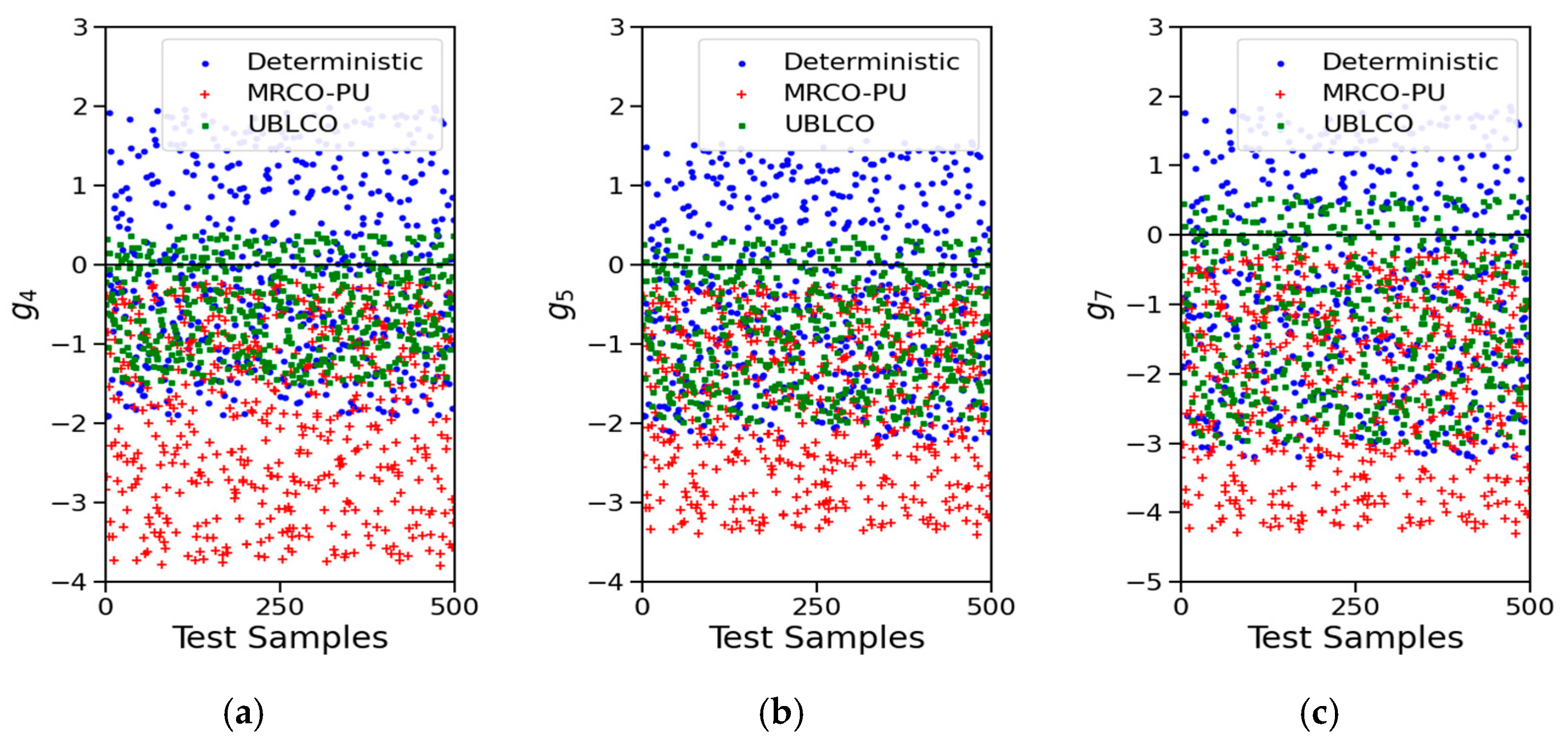
Based on the above mathematical model, robust feasibility verification was conducted for the constraint functions g 4 , g 5 , and g 7 involving uncertain design variables. First, 400 initial sample points were obtained using the LHS method to construct the Kriging model. Then, 100 additional sample points were added according to the EI criterion to improve the model accuracy. Table 6 presents the comparative results of the constraint function robust feasibility under three optimization strategies. The results showed that the deterministic strategy had low robust-feasibility levels of 0.5891, 0.6456, and 0.5739. UBLCO increased the values to 0.8893, 0.9489, and 0.9148, but did not fully satisfy the robust-feasibility requirement. MRCO-PU reached 1.00 for all constraints and fully satisfied the requirement, demonstrating a clear advantage in handling parameter uncertainty.
Figure 10 compares the robust feasibility of three methods across three constraint functions under parameter uncertainty. For deterministic optimization, exceedances of the feasibility threshold are observed for all three constraint functions. With UBLCO, both the frequency and the magnitude of these violations are reduced; occasional exceedances remain. With MRCO-PU, all three constraint functions remain below the feasibility threshold, thereby satisfying robust-feasibility criteria. These findings confirm the effectiveness and robustness of the proposed method for addressing parameter uncertainty.
After verifying robust feasibility, the optimization results of the cutting head were analyzed. Table 7 indicates that, after robust optimization, the average diameter and length of the cutting head show only small variations, ensuring reasonable structural dimensions. The rotational speed increased from 36 r / min in deterministic optimization to 38 r / min . An appropriate increase in speed can improve cutting efficiency, reduce specific energy consumption, shorten the cutting force duration per cut, alleviate wear, and extend pick service life. The swing speed decreased from 1.07 m / min to 1.02 m / min , which helps to stabilize the cutting process and improve rock-breaking efficiency. After applying the proposed MRCO-PU method for robust optimization, the specific energy consumption decreased from 15.02 M J / m 3 to 14.07 M J / m 3 , representing a reduction of 6.3%. The production rate decreased from 72.00 m 3 / h to 71.54 m 3 / h , corresponding to a decrease of 1.3%. Although the production rate was slightly reduced, the MRCO-PU method effectively enhanced the overall robustness of the equipment under parameter uncertainty, demonstrating significant engineering applicability.

6. Conclusions

MRCO-PU is proposed. It integrates CO-WDDI and DL-EI–Kriging to enable multidisciplinary robust optimization for high-end equipment. The main conclusions are as follows:
(1) CO-WDDI performs significantly better than traditional CO in convergence efficiency, computation time, and solution accuracy. Under three different initial points, the numbers of iterations required for convergence were 16, 20, and 34, which are evidently fewer than those of traditional CO, 24, 89, and 40, respectively. The computation times were 4 s, 3 s, and 5 s, each shorter than those of traditional CO, 4 s, 11 s, and 8 s. The optimal objective function values of the three optimization results all reached 8.00, showing high consistency with the given target value. These results demonstrate that the method maintains high stability under different initial conditions.
(2) The DL-EI–Kriging robust optimization model mitigates local uncertainty fluctuations at the discipline level in the inner layer. It also prevents the bidirectional propagation of uncertainty between the system and discipline levels in the outer layer. In this way, the model achieves multi-level uncertainty control. The results of the test function indicate that the EI–Kriging model maintains high fitting accuracy even with a limited number of samples. Moreover, the additional sampling points determined by the EI criterion are concentrated around the predicted optimum, thus ensuring the predictive accuracy of the DL-EI–Kriging model for global optimization.
(3) MRCO-PU is proposed. It integrates CO-WDDI and DL-EI–Kriging into a unified multidisciplinary robust optimization framework. The approach is validated on a mathematical case and an engineering case of a cantilever roadheader cutting head. Evaluation metrics include the objective value, number of iterations, wall-clock time, and robust feasibility. In the mathematical case, deterministic optimization attains a robust feasibility of 0.49, whereas MRCO-PU achieves 1.0, fully meeting the robust-feasibility requirement. In the engineering case, with all constraints robustly feasible, the specific energy consumption decreases by 6.3%, accompanied by a 1.3% reduction in production rate. Despite the slight decline in production rate, MRCO-PU markedly enhances overall robustness and effectively suppresses performance fluctuations under parameter uncertainty, demonstrating strong feasibility and engineering applicability.
Future research will focus on quantifying the inherent uncertainty of surrogate models. It will also explore multidisciplinary robust optimization methods that can concurrently address both parameter and model uncertainty. These efforts aim to enhance the applicability and robustness of the proposed method.

Author Contributions

Conceptualization, Z.W. and Z.Q.; methodology, Z.Q.; validation, Z.Q.; formal analysis, M.C.; investigation, K.Z.; resources, L.L.; data curation, X.L.; writing—original draft preparation, Z.Q.; writing—review and editing, Z.Q.; supervision, Z.W.; project administration, W.C. All authors have read and agreed to the published version of the manuscript.

Funding

This work was supported by the National Natural Science Foundation of China (No. 51975386), Liaoning Province ‘Unveiling and Commanding’ science and technology projects (2022020630-JH1/108), Science and technology research and development program of the China Railway (N2022J014).

Institutional Review Board Statement

Not applicable.

Informed Consent Statement

Not applicable.

Data Availability Statement

The data presented in this study are available on request from the corresponding author. (The datasets generated during and/or analysed during the current study are not publicly available due to Information related to enterprise product processing).

Conflicts of Interest

The authors declare that they have no known competing financial interests or personal relationships that could have appeared to influence the work reported in this paper. The three funding projects mentioned in the paper were all awarded to Professor Zhe Wei, and the funders had no role in the design of the study, in the collection, analysis, or interpretation of data, in the writing of the manuscript, or in the decision to publish the results.

References

  1. Luo, C.; Chen, J.; Liu, Y.; Xiang, H. Enhancing aerodynamic and aeroelastic performance of axial compressor through multi-degree-of-freedom parameterization and data-driven multidisciplinary optimization. Struct. Multidiscip. Optim. 2025, 68, 56. [Google Scholar] [CrossRef]
  2. Yildirim, A.; Jacobson, K.E.; Anibal, J.L.; Stanford, B.K.; Gray, J.S.; Mader, C.A.; Martins, J.R.R.A.; Kennedy, G.J. MPhys: A modular multiphysics library for coupled simulation and adjoint derivative computation. Struct. Multidiscip. Optim. 2025, 68, 15. [Google Scholar] [CrossRef]
  3. Song, Z.; Zheng, X.; Wang, B.; Zhou, K.; Adjei, R.A. Aerodynamic and structural multidisciplinary optimization design method of fan rotors based on blade curvature constraints. Aerosp. Sci. Technol. 2023, 136, 108187. [Google Scholar] [CrossRef]
  4. Sobieszczanski-Sobieski, J. Optimization by Decomposition: A Step from Hierarchic to Non-Hierarchic Systems; Air Force Symposium on Recent Advances in Multidisciplinary Analysis and Optimization; AIAA Paper-94-4325-CP; NASA Technical Reports Server: Washington, DC, USA, 1988. [Google Scholar]
  5. Meng, D.; Zhang, X.; Yang, Y.-J.; Xu, H.; Huang, H.-Z. Interaction balance optimization in multidisciplinary design optimization problems. Concurr. Eng. 2015, 24, 48–57. [Google Scholar] [CrossRef]
  6. Chen, Y.-J.; Huang, H. A novel conceptual design approach for autonomous underwater helicopter based on multidisciplinary collaborative optimization. Eng. Appl. Comput. Fluid Mech. 2024, 18, 2325494. [Google Scholar] [CrossRef]
  7. Zhang, J.; Tian, Y.; Liu, S.; Zhang, W. A novel multidisciplinary hierarchical collaborative optimization of the high-speed pantograph considering the uncertainty of joint clearances. Eng. Optim. 2024, 1–30. [Google Scholar] [CrossRef]
  8. Bao, Y.; Li, H.; Zhao, Y.; Li, L.; Zhang, Z.; Tang, Z. Global–local collaborative optimization method based on parametric sensitivity analysis and application to optimization of compressor blade. Struct. Multidiscip. Optim. 2025, 68, 19. [Google Scholar] [CrossRef]
  9. Mcharek, M.; Azib, T.; Hammadi, M.; Larouci, C.; Choley, J.Y. Multidisciplinary design optimization using knowledge management applied to an electronic throttle. COMPEL-Int. J. Comput. Math. Electr. Electron. Eng. 2020, 39, 353–362. [Google Scholar] [CrossRef]
  10. Sahay, S.; Upputuri, R.; Kumar, N. Optimal power flow-based approach for grid dispatch problems through Rao algorithms. J. Eng. Res. 2023, 11, 100032. [Google Scholar] [CrossRef]
  11. Li, W.; Niu, Y.; He, Y.; Garg, A.; Huang, H.; Gao, L. Multidisciplinary robust design optimization under combined parameter and surrogate model uncertainties: A new computational framework for sparse samples and extreme scenarios. Eng. Comput. 2025, 146, 1–21. [Google Scholar] [CrossRef]
  12. Wu, H.; Du, X. Time- and Space-Dependent Reliability-Based Design With Envelope Method. J. Mech. Des. 2023, 145, 031708. [Google Scholar] [CrossRef]
  13. Thompson, T.; McMullen, R.; Nemani, V.; Hu, Z.; Hu, C. A comparative study of acquisition functions for active learning kriging in reliability-based design optimization. Struct. Multidiscip. Optim. 2025, 68, 51. [Google Scholar] [CrossRef]
  14. Xu, H.W.; Li, W.; Li, M.F.; Hu, C.; Zhang, S.C.; Wang, X. Multidisciplinary robust design optimization based on time-varying sensitivity analysis. J. Mech. Sci. Technol. 2018, 32, 1195–1207. [Google Scholar] [CrossRef]
  15. Taguchi, G. Performance analysis design. Int. J. Prod. Res. 1978, 16, 521–530. [Google Scholar] [CrossRef]
  16. Zhao, Y.; Zhang, X.; Li, D.; Lin, S.; Zhao, X. Robust-Oriented Optimization Design of Dual Three-Phase Slotted Permanent Magnet Hybrid Excitation Generator Considering Manufacturing Tolerances. IEEE Trans. Transp. Electrification 2024, 11, 4561–4573. [Google Scholar] [CrossRef]
  17. Najlaoui, B.; Alghafis, A.; Nejlaoui, M. Robust design of a low cost flat plate collector under uncertain design parameters. Energy Rep. 2023, 10, 2950–2961. [Google Scholar] [CrossRef]
  18. Lin, Q.; Zhou, Q.; Hu, J.; Cheng, Y.; Hu, Z. A Sequential Sampling Approach for Multi-Fidelity Surrogate Modeling-Based Robust Design Optimization. J. Mech. Des. 2022, 144, 111703. [Google Scholar] [CrossRef]
  19. Ma, Y.Z.; Li, C.X.; Wang, Y.Y.; Zhang, Z.Y.; Li, H.S.; Ding, A.N.; Rui, X.T. Robust design optimization of a multi-body system with aleatory and epistemic uncertainty. Reliab. Eng. Syst. Saf. 2024, 245, 110029. [Google Scholar] [CrossRef]
  20. Liu, F.; Yang, S.; Wang, H.; Zhang, W. Multidisciplinary design optimization of an autonomous underwater vehicles based on random uncertainty. Ocean Eng. 2024, 312, 119298. [Google Scholar] [CrossRef]
  21. Zhou, X.; Zhao, W.; Wang, C.; Wang, Y.; Chu, Y. Multidisciplinary Optimization Design of Electric Vehicle X-by-Wire Chassis Integrating Parameter Coupling and Uncertainties. IEEE Trans. Transp. Electrif. 2024, 11, 4765–4777. [Google Scholar] [CrossRef]
  22. Jin, Z.; Sun, X.; Cai, Y.; Tian, X. Robust Collaborative Optimization Design of Plug-In Hybrid Electric Bus Based on 6 Sigma Theory. IEEE Trans. Transp. Electrif. 2024, 10, 10253–10261. [Google Scholar] [CrossRef]
  23. Han, J.; Han, K.; Han, T.; Wang, Y.; Han, Y.; Lin, J. Data-driven distributionally robust optimization of low-carbon data center energy systems considering multi-task response and renewable energy uncertainty. J. Build. Eng. 2025, 102, 111937. [Google Scholar] [CrossRef]
  24. Cheng, J.; Peng, D.; Hu, W.; Liu, Z.; Tan, J. Collaborative robust topology optimization of FGMs considering hybrid bounded uncertainties based on the distance to ideal solution. Compos. Struct. 2024, 341, 118205. [Google Scholar] [CrossRef]
  25. Xiao, S.; Oladyshkin, S.; Nowak, W. Reliability analysis with stratified importance sampling based on adaptive Kriging. Reliab. Eng. Syst. Saf. 2020, 197, 106852. [Google Scholar] [CrossRef]
  26. Zhao, Y.; Li, L.; Li, H.; Liu, X.; Chen, R. An adaptive dual-Kriging method based on parameter sensitivity analysis and application to vibration reduction optimization of helicopter rotor test-bed. Struct. Multidiscip. Optim. 2023, 66, 232. [Google Scholar] [CrossRef]
  27. Xiao, M.; Gao, L.; Shao, X.; Qiu, H.; Jiang, P. A generalized collaborative optimization method and its combination with kriging metamodels for engineering design. J. Eng. Des. 2012, 23, 379–399. [Google Scholar] [CrossRef]
  28. Kroo, I.; Altus, S.; Braun, R.; Gage, P.; Sobieski, I. Multidisciplinary Optimization Methods for Aircraft Preliminary Design; AIAA Paper-94-4325-CP; NASA Technical Reports Server: Washington, DC, USA, 1994. [Google Scholar]
  29. Cao, Z.M.; Zhao, J.; Wang, A. A multidisciplinary Collaborative Optimization Algorithm for Assigning Differential Information According to Weight. Comput. Simul. 2025, 42, 376–426. [Google Scholar]
  30. Yang, C.; Xia, Y. Interval uncertainty-oriented optimal control method for spacecraft attitude control. IEEE Trans. Aerosp. Electron. Syst. 2023, 59, 5460–5471. [Google Scholar] [CrossRef]
  31. Song, R.; Zhou, C.; Rui, J.; Li, H.; Li, J. A volume-ratio index for sensitivity analysis of time-dependent models with interval uncertainty inputs. Aerosp. Sci. Technol. 2025, 160, 110077. [Google Scholar] [CrossRef]
  32. Wang, X.; Wang, R.; Chen, X.; Wang, L.; Geng, X.; Fan, W. Interval prediction of responses for uncertain multidisciplinary system. Struct. Multidiscip. Optim. 2016, 55, 1945–1964. [Google Scholar] [CrossRef]
  33. Wang, L.; Chen, Z.; Yang, G.; Sun, Q.; Ge, J. An interval uncertain optimization method using back-propagation neural network differentiation. Comput. Methods Appl. Mech. Eng. 2020, 366, 113065. [Google Scholar] [CrossRef]
  34. Li, W.; Xiao, M.; Yi, Y.; Gao, L. Maximum variation analysis based analytical target cascading for multidisciplinary robust design optimization under interval uncertainty. Adv. Eng. Inform. 2019, 40, 81–92. [Google Scholar] [CrossRef]
  35. Kim, H.; Michelena, N.; Papalambros, P.; Jiang, T. Target cascading in optimal system design. J. Mech. Des. 2003, 125, 474–480. [Google Scholar] [CrossRef]
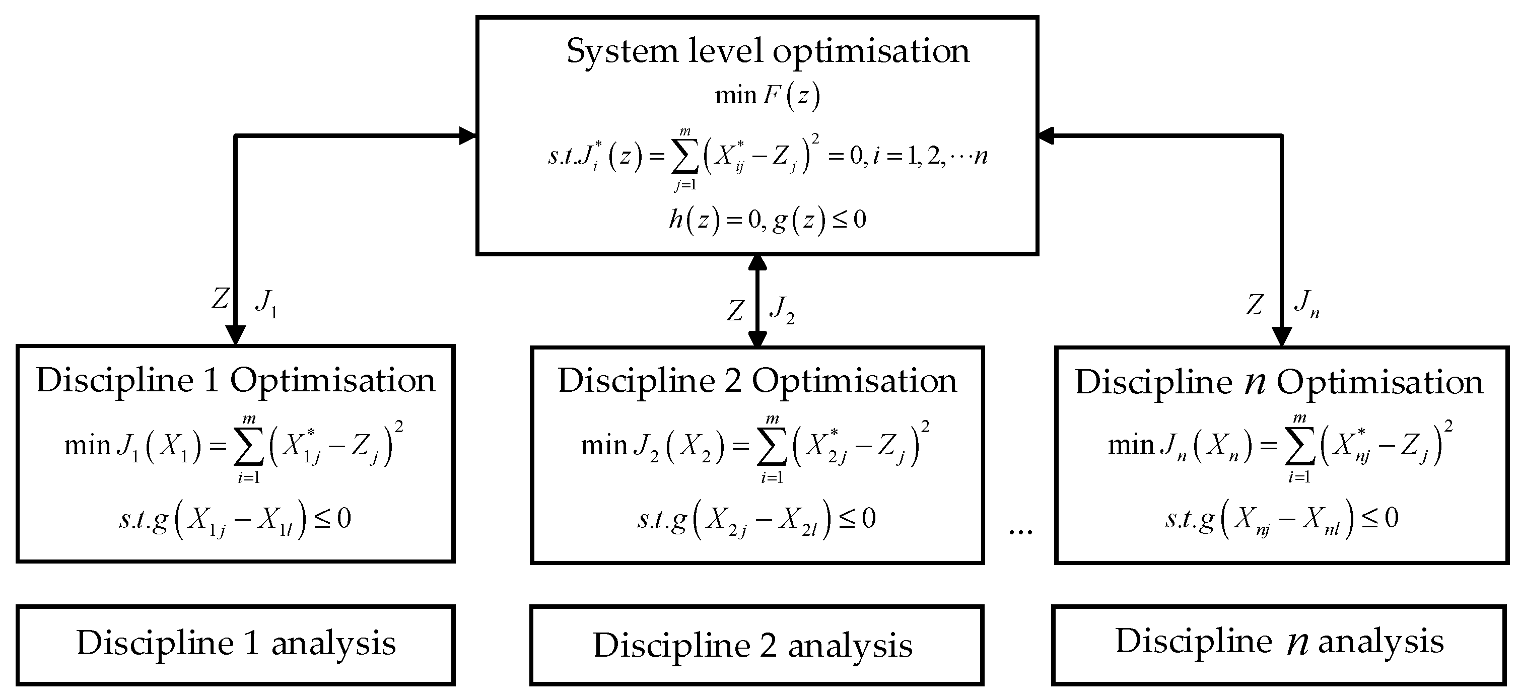
Figure 1. Framework of Collaborative Optimization.
Applsci 15 10549 g001
Figure 2. Optimization approaches: (a) Deterministic design optimization; (b) Robust design optimization.
Applsci 15 10549 g002
Figure 3. Flowchart for the MRCO-PU method.
Applsci 15 10549 g003
Figure 4. True contour map (Dark blue denotes the region of the minimum objective value).
Applsci 15 10549 g004
Figure 5. Kriging model with different sample sizes: (a) 20 sample points; (b) 30 sample points; (c) 40 sample points (Green denotes a medium-to-high range of objective values, while red indicates the highest objective-value range.).
Applsci 15 10549 g005
Figure 6. EI–Kriging with different sample sizes: (a) 20 sample points; (b) 30 sample points; (c) 40 sample points.
Applsci 15 10549 g006
Figure 7. Robust feasibility comparison for the constraint functions: (a) g 1 ; (b) g 2 .
Applsci 15 10549 g007
Figure 8. Assembly of the Cutting Head.
Applsci 15 10549 g008
Figure 9. Schematic of Disciplinary Decomposition for the Cutting Head Optimization Problem.
Applsci 15 10549 g009
Figure 10. Robust feasibility comparison for the constraint functions: (a) g 4 ; (b) g 5 ; (c) g 7 .
Applsci 15 10549 g010
Table 1. Optimization results of ATC, Traditional CO, and CO-WDDI.
Initial PointsOptimization ResultsObjective Function ValueNumber of IterationsComputation Time
ATC(1, 0, 5, 4.38, 8.09)(3.06, 0, 0.06, 7.02, 9.52)7.363512s
(1, 1, 0, 5, 3)(3.29, 0.11, −0.12, 6.65, 8.64)8.6810225s
(−5, 0, 2.5, 26.96, 2.69)(−3.99, 0, 0.17, 9.57, 3.78)6.325714s
Traditional CO(1, 0, 5, 4.38, 8.09)(3.14, 0, −0.28, 7.81, 10)7.52244s
(1, 1, 0, 5, 3)(3.17, 0, −0.25, 7.70, 9.14)7.468911s
(−5, 0, 2.5, 26.96, 2.69)(−3.75, 0, 0, 8.96, 5.86)8.96408s
CO-WDDI(1, 0, 5, 4.38, 8.09)(3.23, 0, 0, 8, 6.72)8.00164s
(1, 1, 0, 5, 3)(3.73, 0, 0, 8, 7.27)8.00203s
(−5, 0, 2.5, 26.96, 2.69)(−3.92, 0, 0, 8, 6.68)8.00345s
Table 2. Robust Feasibility Results of Constraint Functions.
g 1 g 2
Deterministic Optimization0.48560.4989
Robust Optimization (UBLCO)0.92110.9038
Robust Optimization (MRCO-PU)1.01.0
Table 3. Results of Deterministic Optimization and Robust Optimization.
SymbolsDeterministic OptimizationRobust Optimization
(UBLCO)
Robust Optimization
(MRCO-PU)
Design Variables x 1 3.233.143.09
x 2 00.480.66
x 3 00.360.30
y 1 87.877.34
y 2 6.726.847.03
Objective Function Value f 8.008.178.08
Table 4. Design Variables of the Cutting Mechanism.
Design VariablesVariable NamesUnitInitial ValueRange
x 1 Cutting head length Lmm900 800 x 1 1000
x 2 Cutting arm swing speed vm/min0.92 0.8 x 2 1.5
x 3 Average diameter of cutting head Dmm835 600 x 3 1000
x 4 Rotational speed of cutting head nr/min46 20 x 4 50
Table 5. Optimization results for ATC, traditional CO, and CO-WDDI on the Cutting Head case.
Initial PointsOptimization ResultsObjective Function ValueNumber of IterationsComputation Time
ATC(900, 0.92, 835, 46)(901, 0.98, 833, 47)90.554615s
Traditional CO(900, 0.92, 835, 46)(902, 0.96, 832, 45)88.053414s
CO-WDDI(900, 0.92, 835, 46)(899.96, 1.07, 830.8, 6.72)87.02164s
Table 6. Robust Feasibility Results of Constraint Functions.
g 4 g 5 g 7
Deterministic Optimization0.58910.64560.5739
Robust Optimization (UBLCO)0.88930.94890.9148
Robust Optimization (MRCO-PU)1.01.01.0
Table 7. Optimization results of the cutting head.
SymbolsDeterministic OptimizationRobust Optimization
(UBLCO)
Robust Optimization
(MRCO-PU)
Design Variables x 1 899.96901.13898.64
x 2 1.071.011.02
x 3 830.8829.8830.5
x 4 363638
Specific energy consumption H w x 15.0214.2114.07
Productivity Q s x 72.0071.5671.04
Disclaimer/Publisher’s Note: The statements, opinions and data contained in all publications are solely those of the individual author(s) and contributor(s) and not of MDPI and/or the editor(s). MDPI and/or the editor(s) disclaim responsibility for any injury to people or property resulting from any ideas, methods, instructions or products referred to in the content.