Article

Interval Type-II Fuzzy Broad Model Predictive Control Based on the Static and Dynamic Hybrid Event-Triggering Mechanism and Adaptive Compensation for Furnace Temperature in the MSWI Process

1
School of Information Science and Technology, Beijing University of Technology, Beijing 100124, China
2
Beijing Laboratory of Smart Environmental Protection, Beijing 100124, China
3
College of Information Engineering, Dalian Ocean University, Dalian 116023, China
*
Author to whom correspondence should be addressed.
Appl. Sci. 2025, 15(19), 10329; https://doi.org/10.3390/app151910329
Submission received: 27 July 2025 / Revised: 14 September 2025 / Accepted: 19 September 2025 / Published: 23 September 2025

Abstract

Municipal solid waste incineration (MSWI) plays a key role in advancing environmental sustainability. However, the current main furnace temperature control methods are difficult to solve the problems of strong coupling, equipment wear, and frequent disturbances. To solve the above problems, in this article, we propose a static and dynamic hybrid event-triggering mechanism-based interval type-II fuzzy broad adaptive compensation model predictive control (SDHETM-IT2FB-ACMPC). Firstly, a furnace temperature prediction model based on the interval type-2 fuzzy broad learning system (IT2FBLS) is constructed, and the IT2FB-MPC method is obtained, which solve the problem of variable coupling. Secondly, DETM based on historical error information is designed using sliding window method and combined with SETM to form SDHETM to drive the update of control variable to reduce the problem of equipment wear. Finally, the adaptive compensation control law of the adaptive compensation optimization control (ACOC) algorithm can compensate for the influence of the disturbance and the event-triggered mechanism on the control effect, and overcome the problem of frequent disturbances. Experimental results show that the proposed method reduces ISE to 0.2821, IAE to 0.1930, and DEVmax to 6.6269—reductions of 79%, 59%, and 8% compared to traditional NMPC—while cutting control actions by 71%. The results prove that IT2FB-MPC has excellent control performance for furnace temperature, and that SDHETM and ACOC can effectively reduce the triggering times and effectively compensate for the influence caused by disturbances and the lack of control variable updates. The proposed method successfully solves the control difficulties of furnace temperature in the MSWI process.

1. Introduction

In recent years, the production of municipal solid waste (MSW) has surged, leading to the risk of “garbage siege” in many countries [1]. Currently, there are three main mainstream MSW treatment technologies: landfilling, composting, and incineration [2]. Among them, the first two not only pose environmental hazards, but also occupy land resources; moreover, they also have slower processing speeds and lower reduction rates [3]. Municipal solid waste incineration (MSWI) has a fast processing speed and a high reduction rate, but it also has potential environmental hazards in unstable operating conditions. Considering environmental factors and without sufficient advanced technological support, the industry generally prefers to adopt landfilling and composting treatment. However, with the development of advanced technologies such as artificial intelligence and control algorithms, the environmental hazards of MSWI have become controllable [4].
Therefore, MSWI has become a key technology for global environmental governance with its advantages of fast treatment speed and high reduction rate [5,6]. As one of the key controlled variables of the MSWI process, furnace temperature (FT) is directly related to system stability, incineration efficiency, and pollutant generation [7]. At present, an automatic combustion control system is often used to control FT in industrial sites [8], but usually, the instability of MSW calorific value, serious equipment wear, and frequent uncertain disturbance will reduce the actual control effect and even affect the overall stability.
In this regard, scholars have proposed intelligent control algorithms such as fuzzy control [9], neural network control [10], and data-driven model predictive control (DDMPC) [11] for the control process of FT. Among them, DDMPC has demonstrated better control performance in practical applications [12]. As a complex industrial process (CIP), the MSWI mechanism model is complex and uncertain. DDMPC uses a data-driven prediction model to achieve real-time prediction of the future state of the system and optimize the solution of the manipulated variable, which solves the problem of CIP, as it is difficult to establish the mechanism model.
For DDMPC, how to build a prediction model with better performance is one of the research focuses. Scholars have tried to use Gaussian process regression [13], random Forest [14], and artificial neural network (ANN) [15] to construct the prediction model of DDMPC. Among them, the ANN has excellent learning and mapping capabilities [16], which is an effective means of CIP modeling. Considering the model complexity, some shallow ANNs have been widely used in DDMPC in the field of CIP, such as the back propagation neural network [11] and radial basis function neural networks [17]. However, the above methods ignore the strong uncertainty of the actual operation data, which also makes the prediction model itself inaccurate. IT2FNN further combines the interpretation ability of fuzzy logic and fuzzifies the internal parameters [18], so it performs better in practical DDMPC applications [19]. For instance, Wang et al. [20] developed a generalized MPC control system based on IT2FNN, which demonstrated outstanding prediction performance in the ammonia flow control of chemical processes. On the other hand, to pursue higher prediction accuracy, some scholars try to apply deep learning to DDMPC and use deep neural networks (DNNs) such as long short-term memory networks [21] and deep belief networks [22] to build prediction models. Although these works have achieved excellent results, the huge amount of computation of DNNs will bring challenges to the real-time performance of DDMPC, which is unacceptable in the actual control process. Compared with DNNs, the broad learning system (BLS) was first proposed by Chen et al. and reduced most of the computational complexity while retaining the feature extraction ability [23]. On this basis, Han et al. further combined the idea of IT2FNN to construct a broad learning-type model with the ability to deal with uncertainty, named IT2FBLS [24]. Therefore, the IT2FBLS-based prediction model for DDMPC achieves satisfactory prediction accuracy without excessive computational complexity or a complicated network structure.
In addition, equipment wear is also one of the difficult problems in the FT control process. In the field of CIP, scholars generally use an event-triggered mechanism (ETM) to drive the update of control quantities to avoid the impact of equipment wear [25]. For ETM-based MPC systems (ET-MPC), the manipulated variable is usually updated only when the set parameters or the untriggered time reach a certain threshold [26], and this process is also known as static-ETM (SETM). In some previous studies of ET-MPC, SETM can reduce the amount of computation and improve the device lifetime, but the fixed trigger condition may not be able to adapt to the frequent changes of CIP conditions. Ref [27] attempts to introduce internal dynamic variables into SETM, and proposes dynamic ETM (DETM) for the first time. The trigger conditions of DETM change in real time with the system state, which is more flexible and adaptable, so it has excellent performance in some ET-MPC studies [28,29]. Furthermore, Gu et al. [30,31] incorporated sliding window (SW) technology to construct trigger conditions from historical system states, thereby enhancing the robustness of DETM and reducing erroneous triggering caused by sudden disturbances. In fact, the design of DETM usually needs to ensure that the internal state of the MPC system is known [32], but an ANN as a black box model makes it difficult to meet this point.
Facing the above requirements and challenges, this article proposes a static and dynamic hybrid event-triggering mechanism-based interval type-II fuzzy broad adaptive compensation model predictive control (SDHETM-IT2FB-ACMPC) and applies it to FT control of the MSWI process. The innovations of this article are as follows:
(1)
The FT prediction model based on IT2FBLS is proposed to obtain the IT2FB-MPC method, and an online learning algorithm is used to adapt it to the actual operating condition fluctuations.
(2)
SW technology was used to obtain historical error information (HEI) in real time, constructing the HEI-DETM method, which is combined with SETM to form the SDHETM method to prevent the system from false or non-triggering.
(3)
The adaptive compensation optimization control (ACOC) algorithm based on adaptive compensation control law (ACL) and rolling optimization control law (ROL) can compensate for the influence of ETM and disturbance on the control effect, and improve the control performance.
(4)
The convergence and stability of IT2FBLS and SDHETM-IT2FB-ACMPC were theoretically analyzed, and experimental verification based on actual operation data was also conducted.

2. Problem Formulation

2.1. Overview and Characteristic Analysis of the MSWI Process in Terms of FT Control

This article takes an MSWI power plant in Beijing as an example, which adopts the incineration technology of reverse push reciprocating grate furnace, and the specific process flow is shown in Figure 1.
As shown in Figure 1, the MSWI process consists of six stages: solid waste fermentation, solid waste combustion, waste heat exchange, steam power generation, flue gas treatment, and flue gas emission. Among them, solid waste combustion is the key stage of the overall MSWI process, and its stability and efficiency determine the subsequent power generation efficiency, pollutant emission concentration, and other important indicators.
During the solid waste combustion stage, FT is one of the key parameters, and it is directly related to the combustion efficiency and process stability [4]. However, there are numerous process variables that affect FT, and there are extremely tight coupling relationships [10]. Therefore, achieving effective control of the furnace temperature is crucial, and the key lies in selecting the appropriate variables. The steps for selecting the variables are as follows:
First, based on expert knowledge and on-site operation experience, five variables that have a significant impact on the FT are selected as key variables, namely: primary air volume (PV), secondary air volume (SV), feeder speed (FS), drying grate speed (DS), and ammonia injection (AI). Then, the Pearson correlation coefficient (PCC) values between each variable and the FT are calculated separately. Finally, combined with the calculation results and the actual incineration situation, the appropriate variables are selected from the above variables as the control variable. The corresponding PCC value for each variable is shown in the Table 1 below:
Based on the results in Table 1, SV was selected as the controlled variable for SDHETM-IT2FB-ACMPC, while the remaining variables are used as disturbance variables to simulate the actual control environment.

2.2. Model Predictive Control

As a type of discrete control method, MPC repeatedly solves the optimization problem at each control iteration to obtain the optimal control law within a finite time domain at each moment. Therefore, the objective function of the optimization algorithm in MPC is usually set as follows:
J ^ ( t ) = i p = 1 H p e t + i p T w i p y e t + i p + j u = 1 H u Δ u ( t + j u 1 ) T w j u u Δ u ( t + j u 1 )
where H p and H u represent the prediction horizon and control horizon of the system (i.e., the step size of the predicted values and control law set in each iteration, satisfying H p > H u [33]); e t is the deviation between the predicted value and the reference trajectory at time t; Δ u t is the change in the control law at time t; w i p y and w j u u are the weighting parameters of the objective function; and J ^ is the objective function for the system’s online optimization control.

3. Methods

3.1. Method Strategy

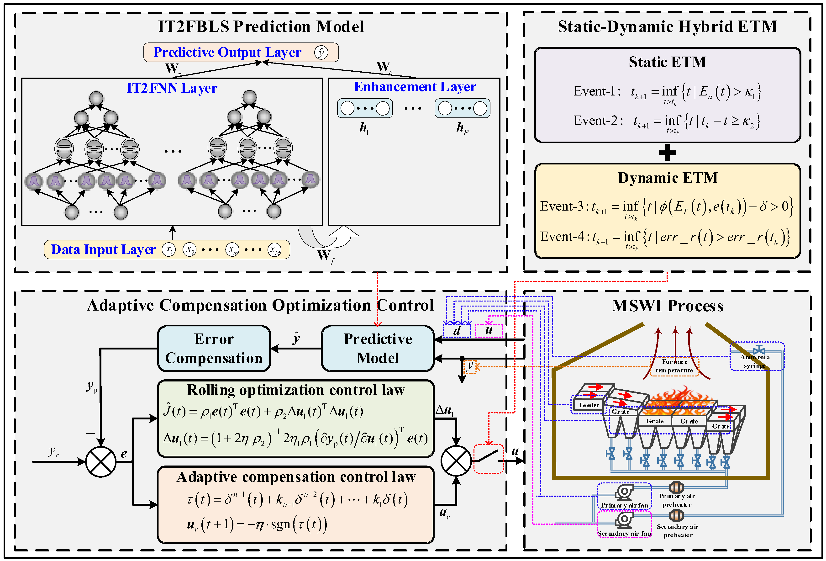
The proposed strategy is shown in Figure 2.
Figure 2 shows that the proposed SDHETM-IT2FB-ACMPC control strategy includes the IT2FBLS prediction model, the ACOC algorithm and the SDHETM algorithm. The functions of each module are as follows.
(1)
IT2FBLS prediction model. The input of this module is the manipulated variable (SV), disturbance variable (PV, FS, DS, AI) and controlled variable (FT) in a past period of time, and the output is the predicted value of the controlled variable in a future period of time (determined by the prediction horizon). This module consists of three parts. Firstly, the IT2FBLS model itself, which is also the core part of the module, is used to calculate the predicted output at future moments based on the obtained historical information. Secondly, the online learning algorithm, which calculates the difference between the predicted output and the expected output and uses the gradient descent method to update the model parameters in real time, thereby avoiding model mismatch. Finally, the prediction error correction, which is specifically proposed for model predictive control, is used to compensate for the prediction sequence with the error of the first item of the prediction sequence, thereby avoiding excessive errors from affecting the actual control effect.
(2)
ACOC algorithm. The input of this module is the error sequence between the compensated prediction sequence and the setpoint value, and the output is the optimal value of the manipulated variable for a future period of time (determined by the control horizon). This module consists of two parts, ROL and ACL. Specifically, the function of ROL is to minimize the objective function based on the existing prediction information, thereby iteratively optimizing the manipulated variable. The function of ACL is to adaptively adjust its size according to the actual control error, thereby compensating for ROL and avoiding the control system being affected by external disturbances.
(3)
SDHETM algorithm. This module uses the design of four triggering events to control the update of manipulated variables. If the system meets a certain triggering event at a certain moment, the optimal value of the manipulated variable is solved through the ACOC algorithm. This process can effectively avoid unnecessary updates of the manipulated variable and ensure that the controlled variable always remains close to the setpoint value.
The operation process of the SDHETM-IT2FB-ACMPC control process is as follows. Firstly, the ACOC algorithm calculates the optimal value of the manipulated variable based on the system error and adjusts the secondary air flow. Then, the IT2FBLS prediction sub-module uses the current and historical manipulated variables, disturbance variables, and controlled variables as inputs to calculate the predicted output of the model. At the same time, the parameter learning sub-module updates the parameters of IT2FBLS in real time to improve the prediction accuracy of the model. Finally, the feedback correction sub-module corrects the predicted output based on the prediction error to obtain the final predicted output. In the next moment, the SDHETM algorithm determines whether to perform the ACOC algorithm based on the current system state information. If so, it uses the aforementioned predicted output to calculate the manipulated variable, thereby forming a closed-loop control.
The computer system used in the paper is Microsoft Windows 11, the CPU is 13th Gen Intel(R) Core (TM) i5-13600KF, and the random-access memory is 32GB. The experiments are programmed with MATLAB 2023a.

3.2. Method Implementation

3.2.1. Interval Type-2 Fuzzy Broad Learning System (IT2FBLS) Predictive Model

IT2FBLS has a strong uncertainty handling capability, which allows it to show a better fitting ability in MSWI applications. Therefore, in this study, IT2FBLS is chosen as the prediction model for FT, and its constructed FT prediction model can be represented by a nonlinear autoregressive exogenous (NARX) system:
y ^ ( t ) = f [ y ( t 1 ) , y ( t 2 ) , , y ( t n y ) , u ( t 1 ) , u ( t 2 ) , , u ( t n u ) , d ( t 1 ) , d ( t 2 ) , , d ( t n u ) ]
This section discusses in detail the pre-training of the IT2FBLS prediction model, the online parameter learning process, and the MPC-oriented prediction error compensation algorithm.
Pre-Training Based on Historical Data
The structure of IT2FBLS is shown in the upper left part of Figure 2 and consists of four parts: the data input layer, the IT2FNN layer, the enhancement layer, and the prediction output layer. Unlike BLS, IT2FBLS replaces the original mapping feature layer with multiple IT2FNN subsystems. The details are as follows.
Data input layer: This layer receives all the sample data at once, which is combined into an input matrix and passed to the subsequent IT2FNN layer. The output of this layer is as follows:
X | N × M = x 1 , x 2 , , x n , , x N T
x n | 1 × M = x n , 1 , x n , 2 , , x n , m , , x n , M
where N is the total number of samples, M is the number of sample features, X is the input matrix, x n is the nth group of samples, and x n , m is the mth input feature of the nth group of samples.
IT2FNN Layer: It is assumed that this layer consists of J IT2FNN subsystems, each of which performs feature extraction on the full sample data and outputs it as a matrix to the augmentation and prediction output layers. The output of this layer is:
Z | N × J = z 1 , z 2 , , z n , , z N T
z n | 1 × J = z 1 n , z 2 n , , z j n , , z J n
The calculation process of the IT2FNN subsystem can be found in [34].
Enhancement layer: It is assumed that this layer consists of P groups of enhancement nodes, each of which receives the output matrix from the IT2FNN layer as input and performs a nonlinear transformation via the tanh function. The output of this layer is:
H | N × P = h 1 , h 2 , , h p , , h P
h p | N × 1 = tanh Z · w p + β p
Predictive output layer: The IT2FBLS constructed in this article is a single-output model, which only predicts the FT in the MSWI process, so the calculation process is as follows:
y ^ | N × 1 = Z · w z + H · w e
where w z and w e are the connection weight vectors of the IT2FNN layer to the output and enhancement layers, respectively.
From Equation (9), it can be seen that IT2FBLS only needs to calculate the connection weights between layers based on the input and output information at the same time to complete the training. For the convenience of subsequent calculations, Equation (9) is rewritten as:
y ^ | N × 1 = Z | H · W = Y · W
where Y and W are the joint matrices of the output and connection weights, respectively.
Since in most cases, the inverse matrix does not exist because of the unequal ranks and columns, the pseudo-inverse matrix is solved by using ridge regression approximation, and the computational procedure is as follows:
W = Y + · y ^
Y + = Y T Y + λ I 1 Y T
where Y + is the pseudo-inverse matrix of Y , λ is the regularization coefficient, and I is the dimensionally compatible identity matrix.
Substituting Equation (12) into Equation (11), the solution formula for W can be obtained as follows.
W = Y T Y + λ I 1 Y T · y ^
Remark 1. 
For IT2FBLS, the internal parameters of the IT2FNN subsystem (membership function center, width, weight) and the connection weights of the IT2FNN layer and the enhancement layer are random values of the appropriate dimension.
Online Learning Based on Real-Time Data
In this article, an online learning algorithm based on real-time data is designed to continuously update the internal parameters of the model according to the predicted effects in the actual FT control in order to gradually adapt to the fluctuation of the operating conditions of the actual process.
The parameters to be updated include the connection weights w p , w z , w e between each layer and the bias term vector β . The process is as follows.
First, we define the performance function based on the prediction error:
E ( t ) = 1 2 ε 2 ( t ) = 1 2 ( y ( t ) y ^ ( t ) ) 2
Furthermore, according to Equation (14), the gradient term of the performance function with respect to the above four parameters can be calculated by the chain derivative rule, as follows:
E t w z , j = E t ε t ε t y ^ t y ^ t w z , j = y ( t ) y ^ ( t ) z j
E t w e , p = E t ε t ε t y ^ t y ^ t w e , p = y ( t ) y ^ ( t ) h p
E t w p , j = E t ε t ε t y ^ t y ^ t h p h p w p , j = y ( t ) y ^ ( t ) w e , p z j 1 h p 2
E t β p = E t ε t ε t y ^ t y ^ t h p h p β p = y ( t ) y ^ ( t ) w e , p 1 h p 2
Finally, combined with the gradient descent algorithm, the online update rules of the above parameters can be obtained:
w z , j t + 1 = w z , j t η z E t w z , j = w z , j t + η z y ( t ) y ^ ( t ) z j
w e , p t + 1 = w e , p t η e E t w e , p = w e , p t + η e y ( t ) y ^ ( t ) h p
w p , j t + 1 = w p , j t η p E t w p , j = w p , j t + η p y ( t ) y ^ ( t ) w e , p z j 1 h p 2
β p t + 1 = β p t η p E t β p = β p t + η p y ( t ) y ^ ( t ) w e , p 1 h p 2
In this article, we do not present the detailed computation of the gradient term.
Remark 2. 
To simplify the design and analysis, the learning rates of parameters   w p , j and β p  are set to the same value. This simplification reduces the complexity of the parameter tuning process while not affecting the convergence and prediction accuracy of the model, which is in line with common practice in training IT2FBLS research [35].
Remark 3. 
In the control process, the number of samples input to IT2FBLS in each iteration is just 1 ( N = 1 ), and it is needed to pay attention to the dimensional changes of the output of each layer.
Predictive Error Compensation
In this article, a prediction error compensation module is added to reduce the prediction error of IT2FBLS in practical applications by calculating the prediction error ε at the current moment, and compensating it for the prediction output at each moment in the prediction horizon H p .
The process is as follows:
ε t = y ^ t y t
y p t + i = y ^ t + i ε t s . t . i = 1 , 2 , , H p

3.2.2. Adaptive Compensation Optimization Control (ACOC)

In this section, the calculation process of the ACOC algorithm is introduced, which includes the ROL and the ACL.
Rolling Optimization Control Law (ROL)
The purpose of the ROL is to solve the optimization problem of MPC: according to the existing prediction information, the objective function is minimized, to iteratively solve the optimal manipulated variable in the finite horizon.
First, we define the following vector:
r ( t ) = y r ( t + 1 ) , y r ( t + 2 ) , , y r ( t + H p ) T
y p ( t ) = y p ( t + 1 ) , y p ( t + 2 ) , , y p ( t + H p ) T
Δ u ROL ( t ) = Δ u ROL ( t ) , Δ u ROL ( t + 1 ) , , Δ u ROL ( t + H u 1 ) T
where H u is the control time domain, r is the set point vector, and Δ u 1 is the vector of the rolling optimization control change.
For the convenience of subsequent derivation, the objective function is defined as:
min J ^ ( t ) = ρ 1 r ( t ) y p ( t ) T r ( t ) y p ( t ) + ρ 2 Δ u ROL ( t ) T Δ u ROL ( t )
To meet the process requirements, the solution time of the manipulated variable should be reduced. The gradient descent method is adopted to achieve the solution of the optimal manipulated variable, which is expressed as:
u ROL ( t + 1 ) = u ROL ( t ) + Δ u ROL ( t ) = u ROL ( t ) η 1 J ^ ( t ) u ROL ( t )
where η 1 0 , 1 is the learning rate of rolling optimization, and the gradient term can be obtained by taking the partial differential of the objective function Equation (28):
J ^ ( t ) u ROL ( t ) = 2 ρ 1 y p ( t ) u ROL ( t ) T r ( t ) y p ( t ) + 2 ρ 2 Δ u ROL ( t )
Substituting Equation (30) into Equation (29), it can be obtained:
Δ u ROL ( t ) = 1 + 2 η 1 ρ 2 1 2 η 1 ρ 1 y p ( t ) u ROL ( t ) T r ( t ) y p ( t )
Remark 4. 
From Equation (31), the Jacobian matrix y p ( t ) / u 1 ( t )  is the key to calculating the control law of rolling optimization. To reduce the volume of computation, the control horizon is set as 1, and solved using the recursive computation of the Jacobian matrix [36].
Adaptive Compensation Control Law (ACL)
In this article, the control system is vulnerable to uncertain disturbance due to the reduction of the number of manipulated variable updates. Therefore, the ACL is designed to improve the actual control effect. The specific implementation process is as follows:
First, a bounded nonlinear mapping (BNM) [37] of the control error is introduced, which is defined as:
δ t = e t λ 1 + e t + e t λ 2 e t
where δ is the mapping error, λ 1 and λ 2 are manually set to positive real numbers.
From Equation (32), the mapping error is infinite when the control error approaches the boundary λ 1 and λ 2 indefinitely. Conversely, if the boundedness of the mapping error is satisfied, then the control error can be ensured to remain within a compact set:
e t = R | e λ 1 , λ 2
Further, filtering error (FE) is introduced to eliminate the effect of small perturbations, defined as:
τ t = δ n 1 t + k n 1 δ n 2 t + + k 1 δ t = k T δ t
where δ t = δ 1 t , , δ n 1 t T , k = k 1 , , k n 1 T is a vector of filter coefficients.
Combined with Equation (34), the computational rule for the ACL is defined as:
u ACL t + 1 = η · sgn τ t
In addition, adjustable weights θ r are introduced, and the optimal manipulated variable under the current moment is obtained by linear summation. It can be described as:
u t + 1 = u ROL t + 1 + θ ACL · u ACL t + 1
Remark 5. 
The ACL in this study is proposed to address the degradation of control performance due to sparse updating of the manipulated variable and frequent disturbances. Moreover, if the ETM is not used to drive the computation of the ACL, the manipulated variable is to be over-updated to some extent, which may lead to a slight degradation of the control performance. This issue will be discussed in the simulation experiments of this article.

3.2.3. Static and Dynamic Hybrid Event-Triggering Mechanism (SDHETM)

In this section, the design process for SDHETM is described in detail, including SETM and HEI-DETM. The two methods are integrated together to update the manipulated variable when either trigger event is met.
SETM (ETM-1)
For SETM, two trigger conditions are designed. First, the absolute control error is introduced, defined as:
e a t = e t = y r t y t
When the absolute control error is greater than a certain threshold, it means that the current control performance does not meet the actual requirements, and the manipulated variable is updated:
Event - 1 : t k + 1 = inf t > t k t | e a t > κ 1
where t k and t k + 1 are the previous and next trigger moments, respectively; and κ 1 indicates the threshold.
In addition, when the time between the controller and the previous trigger moment is bigger than the threshold, the manipulated variable is forced to update:
Event - 1 : t k + 1 = inf t > t k t | e a t > κ 1
where κ 2 indicates the threshold.
Remark 6. 
In fact, in most ETM studies, the trigger condition (Event-2) based on the maximum interval time is designed to ensure the stability of the system.
HEI-DETM (ETM-2)
In this article, the SW method is used to obtain the HEI of the system, and two dynamic trigger conditions are designed based on this. The HEI-DETM process is as follows:
First, the SW is used to obtain historical error information over the past time period:
e ˜ t = e t ρ , e t ρ + 1 , , e t
where e ˜ is used to represent the HEI in the window, and ρ is the preset window size.
Secondly, a variable is defined to quantitatively represent the information in the window, called weighted-HEI. It can be expressed as:
e ˜ 0 t = i = t ρ t w 0 i t e i
where w 0 is the weight of HEI and satisfies i = ρ 0 w 0 i = 1 .
Furthermore, weighted HEI is used to define dynamic trigger conditions as follows:
Event - 3 : t k + 1 = inf t > t k t | ϕ E T t , e t k δ > 0
ϕ E T t , e t k = E T t ς 2 ϖ t e t k ς 2
where E T t = e ˜ 0 t e t k is the difference between weighted-HEI and the control error at the previous trigger time; δ is a small positive real number; and ϖ is the internal dynamic threshold of the event, defined as:
ϖ t = ϖ _ + ϖ ¯ + ϖ _ e E ^ T t 2 s . t . t t k , t k + 1   0 < ϖ _ < ϖ ¯ < 1 > 0
where ϖ _ and ϖ ¯ are the lower and upper bounds of ϖ , respectively; and E ^ T is the relative error information of E T , defined as:
E ^ T t = E T t ς 2 e t k ς 2
where ς is a positive integer, usually set to 1.
A variable is defined again to show the fluctuation of the control effect, called the error fluctuation ratio (EFR). It can be expressed as:
e r r _ r t = W t R t + W t
where R t and W t represent the number of absolute values of control error when the absolute value of historical error is greater than and less than t in the window, respectively. They are denoted as:
R t = R t + 1 , E a t l > E a t R t ,       E a t l E a t W t = W t + 1 , E a t l E a t W t ,       E a t l > E a t s . t . l = 1 , 2 , , ρ
Further, if the EFR at a certain time is bigger than the previous trigger time, the manipulated variable is updated as:
Event - 4 : t k + 1 = inf t > t k t | e r r _ r t > e r r _ r t k
Remark 7. 
For HEI-DETM, HEI is used to reduce the impact of violent disturbance and high-frequency noise. Among them, the size of SW determines the sensitivity of SDHETM to changes in control performance.

3.2.4. Convergence and Stability Analysis

Convergence and stability are key properties of prediction models and control systems, respectively. In this section, the proof procedure of IT2FBLS convergence and the SDHETM-IT2FB-ACMPC stability of the control process are given, respectively.
IT2FBLS Convergence
To ensure the convergence of IT2FBLS, we assume that the higher-order term O ( t ) of the remainder of the Taylor series expansion is bounded, as follows:
1 ψ ε ( t ) A ( t ) < O ( t ) < 1 ψ ε ( t ) + A ( t )
where,
A t = 1 ψ 2 ε 2 ( t ) + ψ ε 2 ( t )
0 < ψ = ψ w z + ψ w e + ψ w p + ψ β < 1
ψ w z = η z θ 1 θ 1 T > 0 , θ 1 = y ^ ( t ) w z
ψ w e = η e θ 2 θ 2 T > 0 θ 2 = y ^ ( t ) w e
ψ w p = η p θ 3 θ 3 T > 0 θ 3 = y ^ ( t ) w p
ψ β = η p θ 4 θ 4 T > 0 θ 4 = y ^ ( t ) β
Then, based on the above assumptions, it can be concluded that for the IT2FBLS system, there is a Lyapunov function based on the prediction error. During the parameter update process of IT2FBLS, the prediction error tends to zero, and the model converges in the time domain. To verify this, we provide the following proof:
First, a Lyapunov function based on the prediction error is defined as follows:
V 1 ( t ) = 1 2 ( y ^ ( t ) y ( t ) ) 2 = 1 2 ε 2 ( t )
The change of the Lyapunov function V 1 can be expressed as:
Δ V 1 ( t ) = V 1 ( t + 1 ) V 1 ( t ) = 1 2 ε 2 ( t + 1 ) ε 2 ( t ) = 1 2 Δ ε ( t ) 2 ε ( t ) + Δ ε ( t )
where Δ ε is the prediction error dynamic, which can be expressed as:
Δ ε ( t ) = ε ( t ) t + O 1 ( t ) = ε ( t ) Φ Φ t T + O 1 ( t ) = ε ( t ) Φ Δ Φ T ε ( t ) Φ O 2 T ( t ) + O 1 ( t ) = ε ( t ) Φ Δ Φ T + O ( t )
where Φ is the vector consisting of each update parameter in IT2FBLS. O 1 ( t ) , O 2 ( t ) and O ( t ) are the higher order terms of the Taylor series expansion residue; and ε ( t ) / Φ and Δ Φ can be denoted as, respectively:
ε ( t ) Φ = ε ( t ) w z , ε ( t ) w e , ε ( t ) w p , ε ( t ) β = y ^ ( t ) w z , y ^ ( t ) w e , y ^ ( t ) w p , y ^ ( t ) β = θ 1 , θ 2 , θ 3 , θ 4
Φ = Δ w z , Δ w e , Δ w p , Δ β
Combined with Equations (19)–(22), each element of Δ Φ can be expressed as:
Δ w z = η z ε ( t ) y ^ ( t ) w z = η z ε ( t ) θ 1
Δ w e = η e ε ( t ) y ^ ( t ) w e = η e ε ( t ) θ 2
Δ w p = η p ε ( t ) y ^ ( t ) w p = η p ε ( t ) θ 3
Δ β = η p ε ( t ) y ^ ( t ) β = η p ε ( t ) θ 4
Combined with Equations (58)–(64), we can get:
Δ ε ( t ) = ε ( t ) η z θ 1 θ 1 T + η e θ 2 θ 2 T + η p θ 3 θ 3 T + η p θ 4 θ 4 T + O ( t ) = ψ ε ( t ) + O ( t )
where ψ is introduced to simplify the expression and satisfy ψ > 0 .
Equation (65) is substituted into Equation (57). Then, from Equations (49)–(55) [17], it can be obtained:
Δ V 1 ( t ) = ψ ε ( t ) + O ( t ) ε ( t ) 1 2 ψ ε ( t ) + 1 2 O ( t ) = ψ ε 2 ( t ) 1 1 2 ψ + 1 2 O 2 ( t ) + ε ( t ) 1 ψ O ( t ) < 1 2 ψ ε 2 ( t ) + 1 2 O 2 ( t ) + ε ( t ) O ( t ) 1 ψ = 1 2 ψ ε 2 ( t ) + 1 2 O ( t ) O ( t ) + 2 ε ( t ) 1 ψ < 1 2 ψ ε 2 ( t ) + 1 2 A ( t ) 1 ψ ε ( t ) A ( t ) + 1 ψ ε ( t ) = 1 2 A 2 ( t ) 1 2 ε 2 ( t ) 1 ψ 2 1 2 ψ ε 2 ( t ) = 1 2 ψ ε 2 ( t ) + ε 2 ( t ) 1 ψ 2 1 2 ε 2 ( t ) 1 ψ 2 1 2 ψ ε 2 ( t ) = 0
In summary, from Equations (49)–(55), Δ V 1 ( t ) < 0 holds and V 1 ( t ) > 0 in Equation (56), therefore, holds:
lim t V 1 ( t ) = lim t ε ( t ) = 0
That is, the prediction error grows gradually to 0 with time and IT2FBLS converges in the time domain.
SDHETM-IT2FB-ACMPC Stability
To ensure the stability of SDHETM-IT2FB-ACMPC, we make the following assumptions:
(1)
The control error of SDHETM-IT2FB-ACMPC is bounded at any time, and it satisfies Equation (33).
(2)
The range of values available for the prediction horizon is sufficiently large, and the weighting factors of the objective function Equation (28) are time-invariant parameters.
(3)
The set threshold of the second trigger condition, Equation (39), is a positive real number with reasonable values.
Then, based on the above assumptions, it can be concluded that for the MSWI process, if the SDHETM-IT2FB-ACMPC method is used, the control system is guaranteed to be nominally asymptotically stable. To verify this, we provide the following proof:
First, the objective function Equation (28) is redefined as follows:
J ^ 1 t = ρ 1 r ( t ) y p ( t ) T r ( t ) y p ( t ) + ρ 2 Δ u * ( t ) T Δ u * ( t )
Then, combined with the above assumption, the ACOC has a (optimal) solution at time t . The resulting sequence of control law increments is denoted as:
Δ u * t = Δ u * t | t , Δ u * t + 1 | t , , Δ u * t + H u 1 | t T
From Equation (69), the control law sequence and corresponding output sequence can be expressed as:
u * t = u * t | t , u * t + 1 | t , , u * t + H u 1 | t T
y * t + 1 = y * t + 1 | t , y * t + 2 | t , , y * t + H p | t T
Further, the sequence of feasible control law increments at time t + 1 is defined as:
Δ u ˜ t + 1 = Δ u ˜ t + 1 | t + 1 Δ u ˜ t + H u 1 | t + 1 Δ u ˜ t + H u | t + 1 Δ u * t + 1 | t Δ u * t + H u 1 | t 0
Then, the feasible control law sequence and the feasible output sequence at time t + 1 are shown as follows:
u ˜ t + 1 = u ˜ t + 1 | t + 1 u ˜ t + H u 1 | t + 1 u ˜ t + H u | t + 1 = u * t + 1 | t u * t + H u 1 | t u * t + H u 1 | t
y ˜ t + 2 = y ˜ t + 2 | t + 1 y ˜ t + H p | t + 1 y ˜ t + H p + 1 | t + 1 = y * t + 2 | t y * t + H p | t y * t + H p | t
Equations (72)–(74) show that the optimization of the objective function J ^ 1 at time t + 1 is feasible. Further, the corresponding (optimal) objective function for Δ u * t is expanded as follows:
J ^ 1 * t = ρ 1 e * t T e * t + ρ 2 Δ u * ( t ) T Δ u * ( t ) = ρ 1 i p = 1 H p e * t + i p | t 2 + ρ 2 j u = 1 H u Δ u * t + j u 1 | t 2
Since the stability of the system is a property under the background of time tending to infinity, the following formula is established in combination with assumption [38]:
e t + i p | t + 1 = e t + i p | t
Then, the (feasible) objective function at time t + 1 can be obtained and denoted as:
J ^ 1 ƛ t + 1 = ρ 1 e ˜ t + 1 T e ˜ t + 1 + ρ 2 Δ u ˜ ( t + 1 ) T Δ u ˜ ( t + 1 ) = ρ 1 i p = 1 H p e ˜ t + i p + 1 | t + 1 2 + ρ 2 j u = 1 H u Δ u ˜ t + j u | t + 1 2 = J ^ * t + ρ 1 e ˜ 2 t + H p + 1 | t ρ 1 e * t + 1 | t 2 ρ 2 Δ u * t | t 2
There are terminal constraints since the maximum prediction range of the system is only for the future H p moments:
e ˜ t + H p + 1 | t = 0
Combined with Equations (77) and (78), this gives:
J ^ 1 ƛ t + 1 J ^ 1 * t = ρ 1 e * t + 1 | t 2 ρ 2 Δ u * t | t 2 0
Further, assume that there exists an optimal solution Δ u * t + 1 to the optimization problem with objective function J 1 at time t + 1 , combined with the properties of MPC; the optimal solution will not be worse than the feasible solution. There exists the following relation:
J ^ 1 * t + 1 J ^ 1 ƛ t + 1
Combined with Equations (79) and (80), this gives:
J ^ 1 * t + 1 J ^ 1 ƛ t + 1 J ^ 1 * t
Combined with above assumption, it can be seen that J ^ 1 * t k + 1 J ^ 1 * t k holds. From Equation (68), the objective function of the optimal solution at any moment is not negative ( J ^ * 0 ).
Therefore, SDHETM-IT2FB-ACMPC is nominally asymptotically stable.

4. Results and Discussion

4.1. Evaluation Indicators

In this experiment, we choose the mean square error (MSE), root mean square error (RMSE), mean absolute error (MAE), and R-squared (R2) as the evaluation indicators to analyze the performance of the prediction model. They are defined as follows:
R M S E = 1 N s n = 1 N s ( y n y ^ n ) 2
M A E = 1 N s n = 1 N s y n y ^ n
R 2 = 1 n ( y n y ^ n ) 2 n ( y n y ¯ ) 2
where y n is the actual value of the sample, y ^ n is the predicted output of the sample, y ¯ is the mean of all sample data, and N s is the total number of samples.
The integral of squared error (ISE), integral of absolute error (IAE) [39] and maximal deviation from set point (Devmax) [40] were chosen as the evaluation indicators to analyze the control performance of the proposed SDHETM-IT2FB-ACMPC. They are defined as follows:
ISE = 1 t f t 0 t = t 0 t f e 2 t
IAE = 1 t f t 0 t = t 0 t f e t
Dev max = max e t 0 , , e t f
where t 0 and t f are the initial time and number of iterations of the controller.

4.2. Dataset Description

The experimental data used in this study are derived from the operation records of a specific day at a real MSWI power plant in Beijing (the operation period is from 8 a.m. to 12 p.m.), with a sampling interval of 1 s. After preprocessing, the final dataset consists of 857 samples, covering six feature variables. Specifically, it includes one controlled variable (FT), four disturbance variables (PV, FS, DS, and AI), and one manipulated variable (SV). The actual ranges of the above process variables are shown in Table 2:

4.3. Prediction Model Experimental Results

This experiment randomly divides the dataset into training set, validation set, and testing set according to the ratio of 2:1:1. Due to space limitation, this section only shows the prediction effect of the testing set. The maximum lag of input and output is set to 1, i.e., the nonlinear model established is denoted as y ^ ( t ) = f [ y ( t 1 ) , u ( t 1 ) , d ( t 1 ) ] . A BPNN [11], FNN [41], IT2FNN [20], and FBLS are used as comparative models for the evaluation of the prediction performance of IT2FBLS. The hyperparameters of the above model are set as follows:
(1)
BPNN: single output model, the number of inputs is 5, the number of hidden layers is 1, the number of hidden layer neurons is 8, the maximum number of convergences is 3000, the convergence error is 0.001, and the parameter learning rate is 0.005.
(2)
FNN: single output model, the number of inputs is 5, the number of fuzzy rules is 20, the parameter learning rate is 0.03, and the updated parameters include: membership function center, membership function width, and consequent connection weights;
(3)
IT2FNN: single output model, the number of inputs is 5, the number of fuzzy rules is 20, the upper and lower bound weighting factor is 0.3, the parameter learning rate is 0.01, and the updated parameters include: the upper and lower bounds of the membership function center, the width of the membership function, and the posterior connection weights.
(4)
FBLS: single output model, the number of inputs is 5, the number of FNN subsystems is 9, the number of subsystem fuzzy rules is 2, the number of enhancement nodes is 17, and the regularization coefficient is 2 × 10⁻³⁰.
(5)
IT2FBLS: single output model, the number of inputs is 5, the number of FNN subsystems is 20, the number of subsystem fuzzy rules is 2, the number of enhancement nodes is 18, and the regularization coefficient is 2 × 10⁻³⁰.
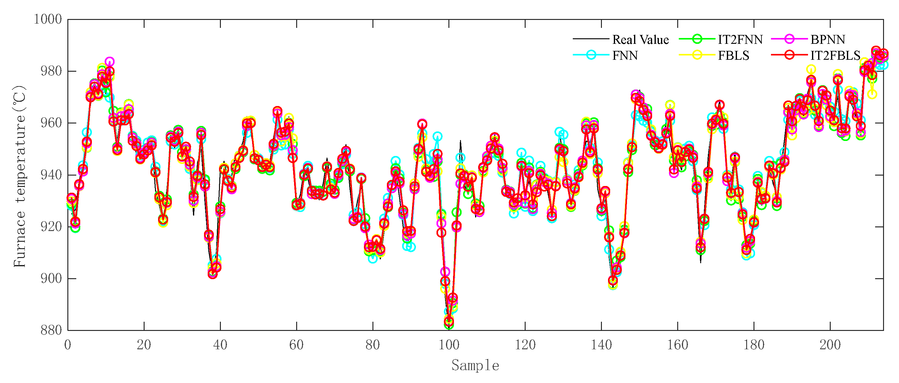
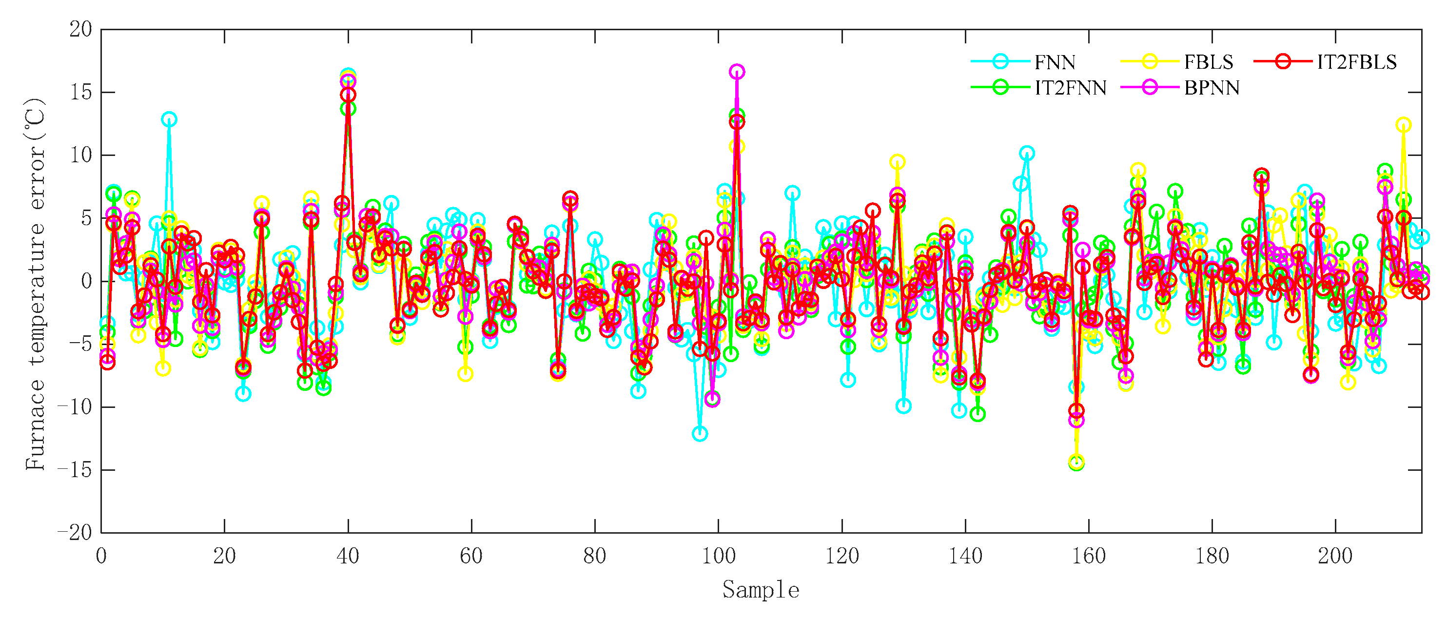
To visualize and compare the prediction performance, the prediction curves and prediction error curves of each model are given, which are shown in Figure 3 and Figure 4:
From Figure 3 and Figure 4, it can be seen that compared with other models, IT2FBLS has the highest prediction accuracy and the smallest prediction error in the vast majority of sample points, and can more accurately predict FT.
Moreover, the performance indicators of each model are shown in Table 3.
From Table 3, all the indicators of IT2FBLS are the minimum values compared to other models. It shows that the prediction error of this model is always kept in a very small range, and it is more suitable for FT predictive control of the MSWI process.

4.4. Tracking Control Experiment Results

To verify the effectiveness and practical performance of the proposed method, a tracking control experiment based on real data is planned to be designed.
In this experiment, the FT setpoint value is the variation between 925 and 935 ° C, the maximum number of iterations was 1200 (the setpoint value is varied between 400 and 800 times), and a Gaussian white noise of 60 dBW is applied to the interference amount. A sample in the data set is randomly selected as the initial value of each process variable.
In this experiment, IT2FBLS-ACN-PID [42], NMPC [11], FNN-MPC [41], IT2FNN-MPC [20], LSTM-MPC [43], FBLS-MPC and I2T2FB-MPC [44] are selected as comparison methods. Additionally, ablation experiments are carried out on SDHETM and ACOC algorithm modules, so as to comprehensively explore the inherent control performance of IT2FB-MPC and the effectiveness of the proposed algorithm. Some of the key hyperparameter settings for each of the above controllers are as follows:
(1)
SDHETM-IT2FB-ACMPC: The prediction horizon is 3, the control horizon is 1, the window size is 8, the static threshold of Event-1 is 0.25, the static threshold of Event-2 is 20, the upper and lower bounds of the dynamic threshold of Event-3 are [0.002, 0.5], the tight set of BNM is (−10, 10), the rolling optimization learning rate is 0.7, the dynamic threshold of event-3 is 0. The learning rates of the connection weights between the IT2FNN layer, the data input layer, and the prediction output layer are 1 × 10⁻⁴, 1 × 10⁻⁴ and 1 × 10⁻⁷, respectively, and the learning rate of the bias term of the enhancement layer is 1 × 10⁻⁷.
(2)
SDHETM-IT2FB-MPC: Same as SDHETM-IT2FB-ACMPC without ACOC-related parameters;
(3)
IT2FB-ACMPC: Same as SDHETM-IT2FB-ACMPC without SDHETM related parameters;
(4)
IT2FB-MPC: Same as SDHETM-IT2FB-ACMPC without ACOC and SDHETM related parameters;
(5)
I2T2FB-MPC: the prediction horizon is 3, the control horizon is 1, and the rolling optimization learning rate is 0.7.
(6)
LSTM-MPC: the prediction horizon is 6, the control horizon is 1, and the rolling optimization learning rate is 0.3.
(7)
FBLS-MPC: the prediction horizon is 6, the control horizon is 1, and the rolling optimization learning rate is 0.3.
(8)
IT2FNN-MPC: the prediction horizon is 6, the control horizon is 1, the rolling optimization learning rate is 0.1, the number of fuzzy rules is 20, the upper and lower bound ratio coefficient is 0.3, and the parameter update learning rate is 0.00001.
(9)
FNN-MPC: the prediction horizon is 2, the control horizon is 1, the learning rate of rolling optimization is 0.15, the number of fuzzy rules is 20, and the learning rate of parameter update is 0.1.
(10)
NMPC: the prediction horizon is 8, the control horizon is 1, and the rolling optimization learning rate is 0.00047.
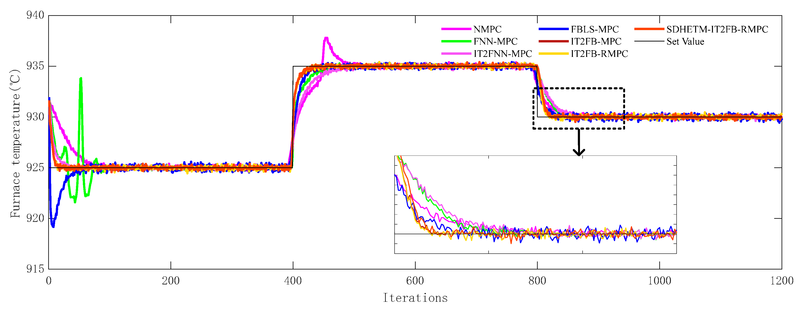
The experimental results are shown in Figure 5, Figure 6, Figure 7, Figure 8, Figure 9 and Figure 10 and Table 4.
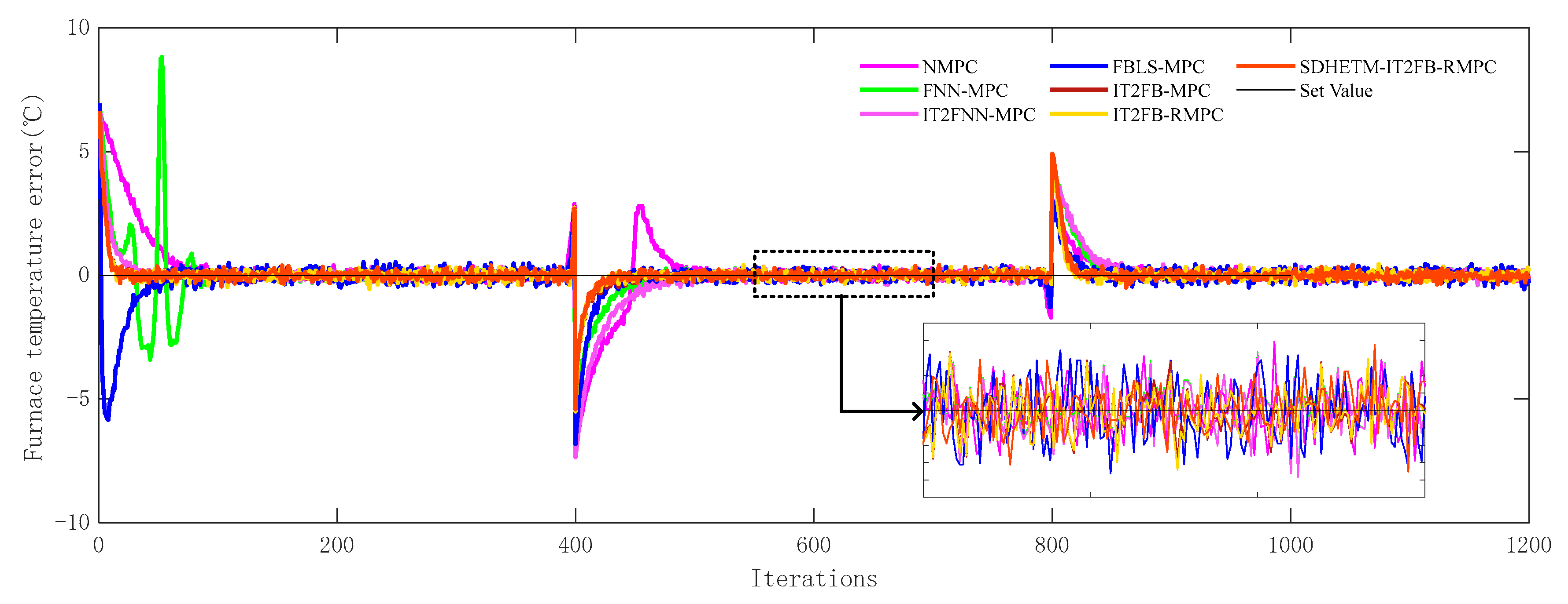
Figure 5 and Figure 6 show that SDHETM-IT2FB-ACMPC can achieve stable control of FT even when the operating conditions change frequently, that is, when the setpoint value changes. Compared with other methods, SDHETM-IT2FB-ACMPC can converge near the setpoint value faster and keep the control error within ±1 °C after the operating condition changes (400, 800th iteration), which meets the actual process requirements, indicating that it has better control performance.
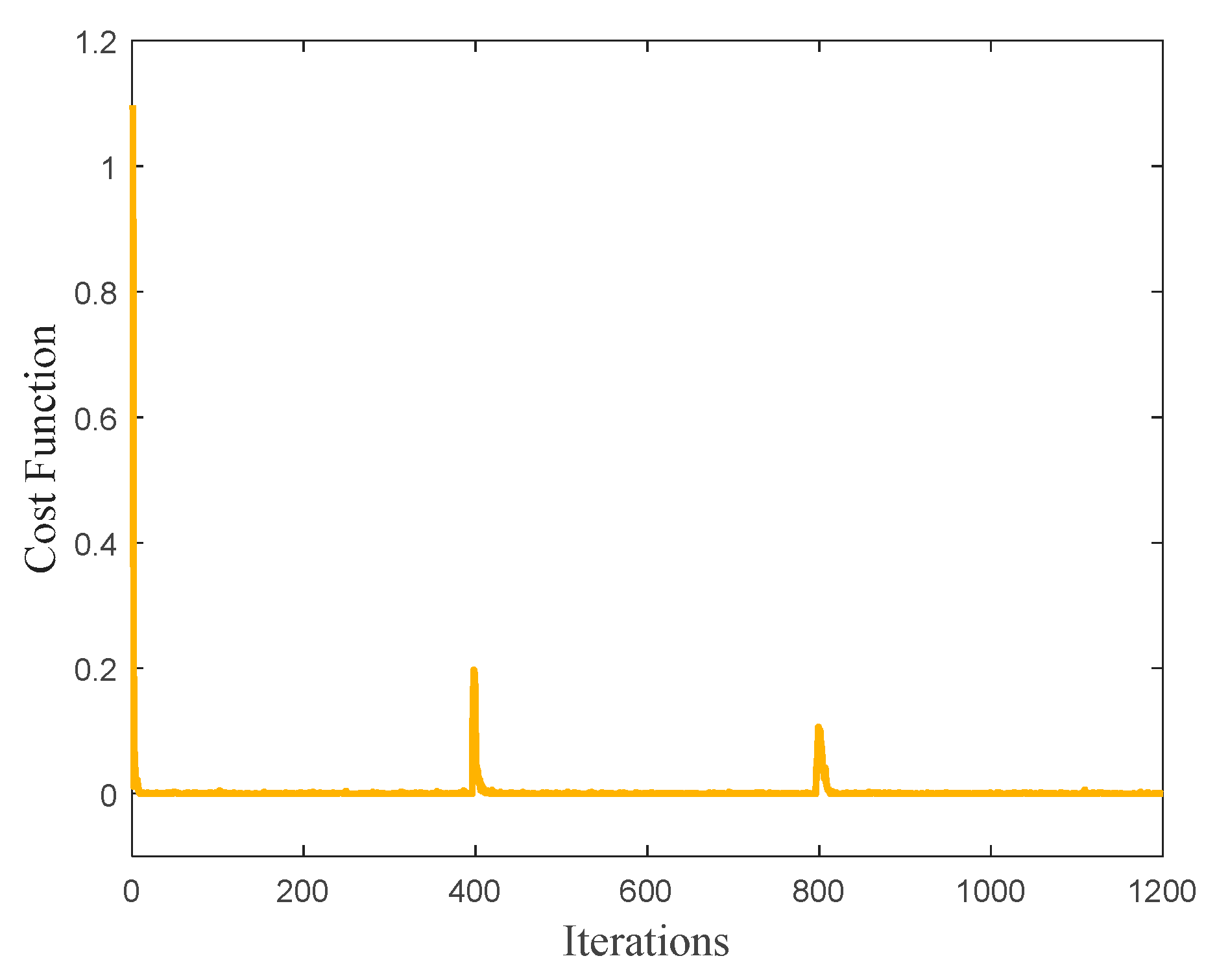
Figure 7 and Figure 8 show that the proposed method can adjust the manipulated variable accurately to realize the automatic control of FT and avoid manual operation. When the set point is unchanged, the ACOC algorithm can converge the value of the objective function to near 0, so as to ensure the stability of the control system. At the same time, Theorem 2 has proved to be a sufficient but not necessary condition.
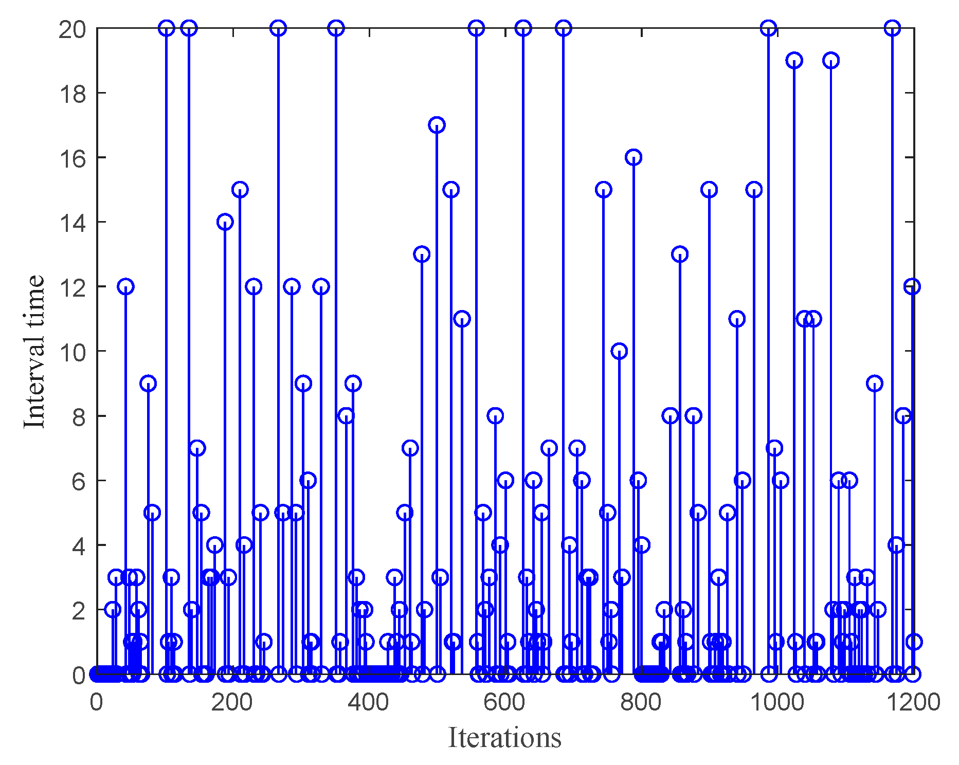
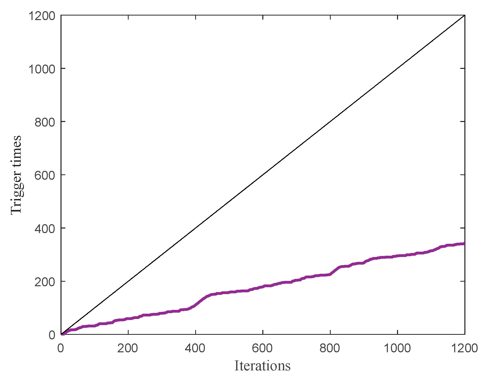
Figure 9 and Figure 10 show that the proposed SDHETM makes the control variable update more frequently only in a short time after the condition changes, while maintaining a long update interval during stable operation. Therefore, SDHETM can effectively reduce the update frequency of manipulated variables to improve the service life of the actuator and avoid additional economic losses.
Moreover, from Table 4, it can be seen that:
(1)
IT2FBLS-ACN-PID, as one of the advanced FT control methods, has good control performance. However, compared with the method proposed in this article, all the indicators are worse, and it has the highest Devmax, indicating that its ability to handle frequent disturbances (i.e., robustness) still needs to be improved.
(2)
Compared with other MPC methods combined with fuzzy logic, the traditional NMPC method has a poor control effect. Only the Devmax values of FNN-MPC and IT2FNN-MPC are slightly higher than those of NMPC. This shows the excellent ability of fuzzy logic to deal with the strong uncertainty of CIP.
(3)
LSTM-MPC, as a type of MPC method based on deep neural networks, demonstrates superior control performance and has lower performance indicators. However, compared with MPC methods based on BLS, its performance indicators are worse, and the control performance still needs to be improved.
(4)
Compared with other MPC methods, the ISE and IAE of the proposed IT2FB-MPC and its improved method are significantly decreased. It indicates that this kind of controller has stronger robustness and adaptive ability, and can ensure that the FT control is more accurate and effective.
(5)
For the IT2FB-MPC and its improved method proposed in this article, Devmax is the same value. The reason may be that when the initial value of each variable and the prediction model are the same, the initial value of the actual FT value is also the same, resulting in the same Devmax value.
(6)
I2T2FB-MPC, as one of the advanced methods in the field of IT2FB-MPC, possesses excellent control performance. However, ISE and IAE are still lower than those of IT2FB-ACMPC, indicating that the ACOC algorithm effectively compensates for the impact of frequent disturbances on the controller, successfully enhancing its robustness and control accuracy.
(7)
IT2FB-ACMPC has the smallest ISE and IAE values, and Devmax remains unchanged, which indicates that the proposed ACOC algorithm can still eliminate some large error points and improve the overall control effect when ETM is not used to drive the control variable update.
(8)
Compared with IT2FB-MPC, the ISE and IAE of SDHETM-IT2FB-MPC are only increased by about 10.2% and 5%, respectively, Devmax remains unchanged, and the number of triggers is reduced by about 69.2%. This indicates that the proposed SDHETM can not only sacrifice a small part of control performance, but also reduce the trigger times. The proposed method greatly reduces the number of control variable updates and improves the service life of the equipment.
(9)
For SDHETM-IT2FB-ACMPC, compared with SDHETM-IT2FB-MPC, the number of triggers is reduced by 27 times, about 7.3%; ISE and IAE are reduced by about 2.8% and 3.7%, respectively, while Devmax remains unchanged. It shows that when ETM is used to drive the control update, the ACL can effectively improve the control effect of IT2FB-MPC, while ensuring that the number of control updates is at a low level.

4.5. Ablation Experiment for SDHETM

To further explore SDHETM and the separate roles of its modules, this article designed an ablation experiment for SDHETM. IT2FB-MPC is selected as the controller, and the experimental settings are consistent with Section 4.3. The comparison methods include IT2FB-ACMPC with only SETM [43], DETM [30], and HEI-DETM. The comparison indicators include ISE, IAE, Devmax and triggering times.
Table 5 shows that:
(1)
For SETM, although performance indicators can be guaranteed not to rise greatly, there is still room for further decline in trigger times. It indicates that the method appropriately increases the update times of control quantities in order to maintain the original control performance. However, this cannot guarantee the maximum extension of the equipment life in the actual control process.
(2)
For DETM, although the trigger times are significantly reduced, the corresponding performance indicators are significantly increased. It indicates that these methods sacrifice more control performance to reduce the number of control variable updates. This may affect the stability of the actual control process and cause economic losses.
(3)
Compared with other DETMs, the corresponding performance indicators of the HEI-DETM proposed in this article are significantly decreased. Thus, although the number of triggers is slightly increased, the improvement of control performance is more obvious.
(4)
Compared with Baseline and other methods, the ISE and IAE values of SDHETM proposed in this article only increase by 9.3% and 2%, respectively, while Devmax remains unchanged. Although the trigger times are the highest value, it is still reduced by 71.4% compared with Baseline, with only 343 trigger times.
Table 5. Comparison of performance indicators of IT2FB-ACMPC corresponding to each ETM.
ControllerISEIAEDevmaxTriggering Times
IT2FB-ACMPC (Baseline)0.28210.19306.62691200
SETM-IT2FB-ACMPC [43]0.3178 (↑12.7%)0.1980 (↑2.6%)6.6269 (---)373 (↓68.9%)
DETM-IT2FB-ACMPC [30]0.3318 (↑17.6%)0.2286 (↑18.5%)6.6269 (---)330 (↓72.5%)
HEI-DETM-IT2FB-ACMPC0.3093 (↑9.6%)0.2049 (↑6.2%)6.6269 (---)363 (↓69.8%)
SDHETM-IT2FB-ACMPC0.3084 (↑9.3%)0.1969 (↑2%)6.6269 (---)343 (↓71.4%)
Note: The best result and the controller with the best overall performance are highlighted in bold. Smaller values represent the best performance in each indicator. “↑”, “↓”, and “---" respectively indicate that the corresponding indicators of the controller have increased, decreased, or remained unchanged compared to the baseline.
In summary, the experimental results show that SDHETM fully combines the advantages of HEI-DETM and SETM. It can reduce the number of control variable updates while not affecting the original control effect as much as possible. Thus, it is more suitable for application in the actual MSWI process (including other CIP) and improves the service life of incineration equipment.

5. Conclusions

In this article, an FT control method for SDHETM-IT2FB-MPC is designed. This method can reduce the reliance on manual operation, improve the level of automation and intelligence, and enhance the FT control effect as well as the service life of the equipment. The experimental results show: (1) For IT2FBLS, compared with the traditional BPNN, its MSE, RMSE, and MAE are reduced by 37.2%, 15.9%, and 19.7%, respectively, and R2 is increased by 1.4%; (2) For IT2FB-ACMPC, compared with the traditional NMPC, its ISE, IAE, and DEVmax are reduced by 79%, 59%, and 8%, respectively; (3) For SDHETM, its control variable update times of the system are reduced by 71%. From these results, it can be seen that IT2FBLS can accurately predict future changes of FT, and the proposed controller has excellent control performance, which can significantly reduce the number of control updates and maximize the control performance of FT.
Although the proposed method has excellent effects, SDHETM still has limitations in application: (1) The SDHETM algorithm includes a large number of hyperparameters, and when applied to different scenarios, they need to be adjusted one by one according to the actual situation; (2) The historical information of system control errors needs to be saved, and the amount of information is proportional to the sliding window size, which has high requirements for storage devices in industrial sites.
For furnace temperature control, future research directions include: (1) Designing a prediction model for multiple operating conditions to fully overcome the process fluctuations of MSWI and thereby improve the prediction accuracy of FT; (2) Designing adaptive algorithms for a large number of hyperparameters in the control system to avoid errors caused by excessive manual operations; (3) Applying the proposed algorithm to the digital twin platform of the MSWI process to facilitate the implementation of the algorithm in actual industrial application.

Author Contributions

Conceptualization, J.T.; Methodology, J.T.; Software, B.W. and J.R.; Validation, J.R.; Formal analysis, J.T.; Investigation, B.W.; Resources, B.W. and J.R.; Data curation, B.W.; Writing-original draft, B.W.; Writing-review and editing, J.T. and W.W.; Visualization, B.W.; Supervision, J.T. and W.W.; Project administration, J.T. All authors have read and agreed to the published version of the manuscript.

Funding

This work was supported in part by the General Scientific Research Projects of Liaoning Province Science and Technology Joint Plan Project under Grant 2024JH2/102600083, and in part by Liao-ning Provincial Department of Education under Grant JYTMS20230489.

Institutional Review Board Statement

Not applicable.

Informed Consent Statement

Not applicable.

Data Availability Statement

The data presented in this study are available on request from the corresponding author.

Conflicts of Interest

The authors declare no conflict of interest.

Abbreviations

NumberAbbreviationsMeanings
1MSWMunicipal Solid Waste
2MSWIMunicipal Solid Waste Incineration
3FTFurnace Temperature
4DDMPCData-driven Model Predictive Control
5CIPComplex Industrial Process
6ANNArtificial Neural Network
7IT2FNNInterval Type-II Fuzzy Neural Network
8DNNDeep Neural Network
9BLSBroad Learning System
10IT2FBLSInterval Type-II Fuzzy Broad Learning System
11ETMEvent-triggering Mechanism
12SETMStatic Event-triggering Mechanism
13DETMDynamic Event-triggering Mechanism
14SWSliding Window
15SDHETMStatic and Dynamic Hybrid Event-triggering Mechanism
16HEIHistorical Error Information
17ACLAdaptive Compensation Control Law
18ROLRolling Optimization Control Law
19ACOCAdaptive Compensation Optimization Control
20PCCPearson Correlation Coefficient
21PVPrimary Air Volume
22SVSecondary Air Volume
23FSFeeder Even Speed
24DSDrying Grate Even Speed
25AIAmmonia Injection
26NARXNonlinear Autoregressive Exogenous
27BNMBounded Nonlinear Mapping
28FEFiltering Error
29EFRError Fluctuation Ratio
30MSEMean Square Error
31RMSERoot Mean Square Error
32MAEMean Absolute Error
33R2R-squared
34ISEIntegral of Squared Error
35IAEIntegral of Absolute Error
36DevmaxMaximal Deviation from Setpoint

References

  1. Gómez-Sanabria, A.; Kiesewetter, G.; Klimont, Z.; Schoepp, W.; Haberl, H. Potential for future reductions of global GHG and air pollutants from circular waste management systems. Nat. Commun. 2022, 13, 106. [Google Scholar] [CrossRef] [PubMed]
  2. Ding, Y.; Zhao, J.; Liu, J.-W.; Zhou, J.; Cheng, L.; Zhao, J.; Shao, Z.; Iris, Ç.; Pan, B.; Li, X.; et al. A review of China’s municipal solid waste (MSW) and comparison with international regions: Management and technologies in treatment and resource utilization. J. Clean. Prod. 2021, 293, 126144. [Google Scholar] [CrossRef]
  3. Qiao, J.F.; Guo, Z.H.; Tang, J. Dioxin emission concentration measurement approaches for municipal solid wastes incineration process: A survey. Acta Anat. Sin. 2020, 46, 1063–1089. [Google Scholar] [CrossRef]
  4. Tang, J.; Xia, H.; Yu, W.; Qiao, J.F. Research status and prospects of intelligent optimization control for municipal solid waste incineration process. Acta Anat. Sin. 2023, 49, 2019–2059. [Google Scholar] [CrossRef]
  5. Yang, D.K.; Kow, K.; Wang, W.L.; Meredith, W.; Zhang, G.L.; Mao, Y.P.; Xu, M.X. Co-treatment of municipal solid waste incineration fly ash and alumina-/silica-containing waste: A critical review. J. Hazard. Mater. 2024, 479, 135677. [Google Scholar] [CrossRef]
  6. Chuai, X.; Yang, Q.H.; Zhang, T.T.; Zhao, Y.C.; Wang, J.; Zhao, G.D.; Cui, X.Z.; Zhang, Y.L.; Zhang, T.L.; Xiong, Z.; et al. Speciation and leaching characteristics of heavy metals from municipal solid waste incineration fly ash. Fuel 2022, 328, 125338. [Google Scholar] [CrossRef]
  7. Ding, H.X.; Qiao, J.F.; Huang, W.M.; Yu, T. Event-triggered online learning fuzzy-neural robust control for furnace temperature in municipal solid waste incineration process. IEEE Trans. Autom. Sci. Eng. 2024, 21, 1201–1213. [Google Scholar] [CrossRef]
  8. Wang, T.Z.; Tang, J.; Xia, H.; Yang, C.L.; Yu, W.; Qiao, J.F. Data-driven multi-objective intelligent optimal control of municipal solid waste incineration process. Eng. Appl. Artif. Intell. 2024, 137A, 109157. [Google Scholar] [CrossRef]
  9. Shen, K.; Lu, J.D.; Li, Z.H.; Liu, G. An adaptive fuzzy approach for the incineration temperature control process. Fuel 2005, 84, 1144–1150. [Google Scholar] [CrossRef]
  10. Tian, H.; Tang, J.; Xia, H.; Yu, W.; Qiao, J.F. Bayesian optimization-based interval type-2 fuzzy neural network for furnace temperature control. IEEE Trans. Ind. Inf. 2025, 21, 505–514. [Google Scholar] [CrossRef]
  11. Wang, B.K.; Tang, J.; Xia, H.; Tian, H.; Wang, T.Z.; Wu, Z.W. Furnace Temperature Control for MSWI Process Based on Neural Network Predictive Controller. In Proceedings of the 2024 36th Chinese Control and Decision Conference (CCDC), Xi’an, China, 25–27 May 2024; pp. 1731–1736. [Google Scholar] [CrossRef]
  12. Hu, K.C.; Yan, A.J.; Wang, D.H. Nonlinear model predictive control of furnace temperature for a municipal solid waste incineration process. Control Theory Appl. 2024, 41, 2023–2032. [Google Scholar] [CrossRef]
  13. Liu, M.; Sun, Z.Q.; Hu, R.; Xia, Y.Q. Safety enhancement for nonlinear systems via learning-based model predictive control with Gaussian process regression. Neurocomputing 2024, 591, 127706. [Google Scholar] [CrossRef]
  14. Smarra, F.; Jain, A.; Rubeis, T.; Ambrosini, D.; D’Innocenzo, A.; Mangharam, R. Data-driven model predictive control using random forests for building energy optimization and climate control. Appl. Energy 2018, 226, 1252–1272. [Google Scholar] [CrossRef]
  15. Han, H.G.; Qiao, J.F.; Chen, Q.L. Model predictive control of dissolved oxygen concentration based on a self-organizing RBF neural network. Control Eng. Pract. 2012, 20, 465–476. [Google Scholar] [CrossRef]
  16. Fei, J.T.; Liu, L.H.J. Real-time nonlinear model predictive control of active power filter using self-feedback recurrent fuzzy neural network estimator. IEEE Trans. Ind. Electron. 2022, 69, 8366–8376. [Google Scholar] [CrossRef]
  17. Xie, S.W.; Xie, Y.F.; Huang, T.W.; Gui, W.H.; Yang, C.H. Generalized predictive control for industrial processes based on neuron adaptive splitting and merging RBF neural network. IEEE Trans. Ind. Electron. 2019, 66, 1192–1202. [Google Scholar] [CrossRef]
  18. Liu, X.; Zhao, T.Y.; Cao, J.T.; Li, P. Design of an interval type-2 fuzzy neural network sliding mode robust controller for higher stability of magnetic spacecraft attitude control. ISA Trans. 2023, 137, 144–159. [Google Scholar] [CrossRef]
  19. Tafti, B.; Teshnehlab, M.; Ahmadieh, M.K. Recurrent interval type-2 fuzzy wavelet neural network with stable learning algorithm: Application to model-based predictive control. Int. J. Fuzzy Syst. 2020, 22, 351–367. [Google Scholar] [CrossRef]
  20. Wang, M.X.; Wang, Y.F.; Chen, G. Interval type-2 fuzzy neural network based constrained GPC for NH3 flow in SCR de-NOx process. Neural. Comput. Appl. 2021, 33, 16057–16078. [Google Scholar] [CrossRef]
  21. Huang, K.K.; Wei, K.; Li, F.B.; Yang, C.H.; Gui, W.H. LSTM-MPC: A Deep Learning Based Predictive Control Method for Multimode Process Control. IEEE Trans. Ind. Electron. 2023, 70, 11544–11554. [Google Scholar] [CrossRef]
  22. Wang, G.M.; Jia, Q.S.; Qiao, J.F.; Bi, J.; Zhou, M.C. Deep Learning-Based Model Predictive Control for Continuous Stirred-Tank Reactor System. IEEE Trans. Neural Netw. Learn. Syst. 2021, 32, 3643–3652. [Google Scholar] [CrossRef]
  23. Chen, C.L.P.; Liu, Z.L. Broad Learning System: An Effective and Efficient Incremental Learning System Without the Need for Deep Architecture. IEEE Trans. Neural Netw. Learn. Syst. 2018, 29, 10–24. [Google Scholar] [CrossRef] [PubMed]
  24. Han, H.G.; Liu, Z.; Liu, H.X.; Qiao, J.F.; Chen, C.L.P. Type-2 Fuzzy Broad Learning System. IEEE Trans. Cybern. 2022, 52, 10352–10363. [Google Scholar] [CrossRef]
  25. Ding, H.X.; Qiao, J.F.; Huang, W.M.; Yu, T. Cooperative event-triggered fuzzy-neural multivariable control with multitask learning for municipal solid waste incineration process. IEEE Trans. Ind. Inf. 2024, 20, 765–774. [Google Scholar] [CrossRef]
  26. Boruah, N.; Roy, B.K. Event triggered nonlinear model predictive control for a wastewater treatment plant. J. Water Process Eng. 2019, 32, 100887. [Google Scholar] [CrossRef]
  27. Girard, A. Dynamic triggering mechanisms for event-triggered control. IEEE Trans. Autom. Control 2015, 60, 1992–1997. [Google Scholar] [CrossRef]
  28. Shi, T.; Shi, P.; Wu, Z.G. Dynamic Event-Triggered Asynchronous MPC of Markovian Jump Systems with Disturbances. IEEE Trans. Cybern. 2022, 52, 11639–11648. [Google Scholar] [CrossRef]
  29. Wang, C.C.; Geng, Q.; Liu, F.C.; Fu, L.N. Observer-based MPC for fuzzy cyber–physical system with hybrid attacks via a dynamic event-triggered mechanism. J. Frankl. Inst. 2024, 361, 106772. [Google Scholar] [CrossRef]
  30. Gu, Z.; Yue, D.; Park, J.H.; Xie, X.P. Memory-event-triggered fault detection of networked IT2 T-S fuzzy systems. IEEE Trans. Cybern. 2023, 53, 743–752. [Google Scholar] [CrossRef]
  31. Gu, Z.; Yue, D.; Ahn, C.K.; Yan, S.; Xie, X.P. Segment-weighted information-based event-triggered mechanism for networked control systems. IEEE Trans. Cybern. 2023, 53, 5336–5345. [Google Scholar] [CrossRef] [PubMed]
  32. Rong, N.N.; Wang, B.H.; Zhang, X.W.; Ji, Y. Dynamic event-based model predictive control of IT2 T-S fuzzy system. IEEE Trans. Circuits Syst. II-Exp. Briefs 2024, 71, 692–696. [Google Scholar] [CrossRef]
  33. Wang, Y.J.; Huang, J.Q.; Zhou, W.X.; Lu, F.; Xu, W.H. Neural network-based model predictive control with fuzzy-SQP optimization for direct thrust control of turbofan engine. Chin. J. Aeronaut. 2022, 35, 59–71. [Google Scholar] [CrossRef]
  34. Han, H.G.; Wang, C.Y.; Sun, H.Y.; Qiao, J.F. Data-based robust model predictive control for wastewater treatment process. J. Process Control 2022, 118, 115–125. [Google Scholar] [CrossRef]
  35. Tian, H.; Tang, J.; Aljerf, L.; Wang, T.Z.; Qiao, J.F. Furnace temperature control based on interval type-2 fuzzy broad learning system for municipal solid waste incineration process. Expert Syst. Appl. 2025, 280, 127530. [Google Scholar] [CrossRef]
  36. Noriega, J.R.; Wang, H. A direct adaptive neural-network control for unknown nonlinear systems and its application. IEEE Trans. Neural Netw. 1998, 9, 27–34. [Google Scholar] [CrossRef]
  37. Han, H.G.; Yang, F.F.; Sun, H.Y.; Qiao, J.F. Robust type-2 fuzzy neural control for wastewater treatment process with external disturbances. IEEE Trans. Autom. Sci. Eng. 2024, 21, 7230–7241. [Google Scholar] [CrossRef]
  38. Xiao, H.Z.; Chen, C.L.P. Incremental updating multirobot formation using nonlinear model predictive control method with general projection neural network. IEEE Trans. Ind. Electron. 2019, 66, 4502–4512. [Google Scholar] [CrossRef]
  39. Han, H.G.; Liu, Z.; Liu, H.X.; Qiao, J.F. Knowledge-Data-Driven Model Predictive Control for a Class of Nonlinear Systems. IEEE Trans. Syst. Man Cybern. Syst. 2021, 51, 4492–4504. [Google Scholar] [CrossRef]
  40. Zhao, J.K.; Dai, H.L.; Wang, Z.Y.; Chen, C.; Cai, X.W.; Song, M.Y.; Guo, Z.C.; Zhang, S.; Wang, X.G.; Geng, H.Y. Self-organizing modeling and control of activated sludge process based on fuzzy neural network. J. Water Process Eng. 2023, 53, 103641. [Google Scholar] [CrossRef]
  41. Han, H.G.; Liu, Z.; Qiao, J.F. Fuzzy Neural Network-Based Model Predictive Control for Dissolved Oxygen Concentration of WWTPs. Int. J. Fuzzy Syst. 2019, 21, 1497–1510. [Google Scholar] [CrossRef]
  42. Tian, H.; Tang, J.; Xia, H.; Wang, T.Z.; Yu, W.; Qiao, J.F. Furnace Temperature Control Using IT2FBLS-based Reinforcement Learning PID for MSWI Process. Acta Automat. Sin. 2025, 51, 1626–1641. [Google Scholar] [CrossRef]
  43. Qiao, J.F.; Sun, J.; Meng, X. Event-triggered adaptive model predictive control of oxygen content for municipal solid waste incineration process. IEEE Trans. Autom. Sci. Eng. 2024, 21, 463–474. [Google Scholar] [CrossRef]
  44. Wang, B.K.; Tang, J.; Tian, H.; Yu, W.; Qiao, J.F. Improved Interval Type-II Fuzzy Broad MPC Method for Furnace Temperature of Municipal Solid Waste Incineration Process. IEEE Trans. Fuzzy Syst. 2025; to be published. [Google Scholar] [CrossRef]
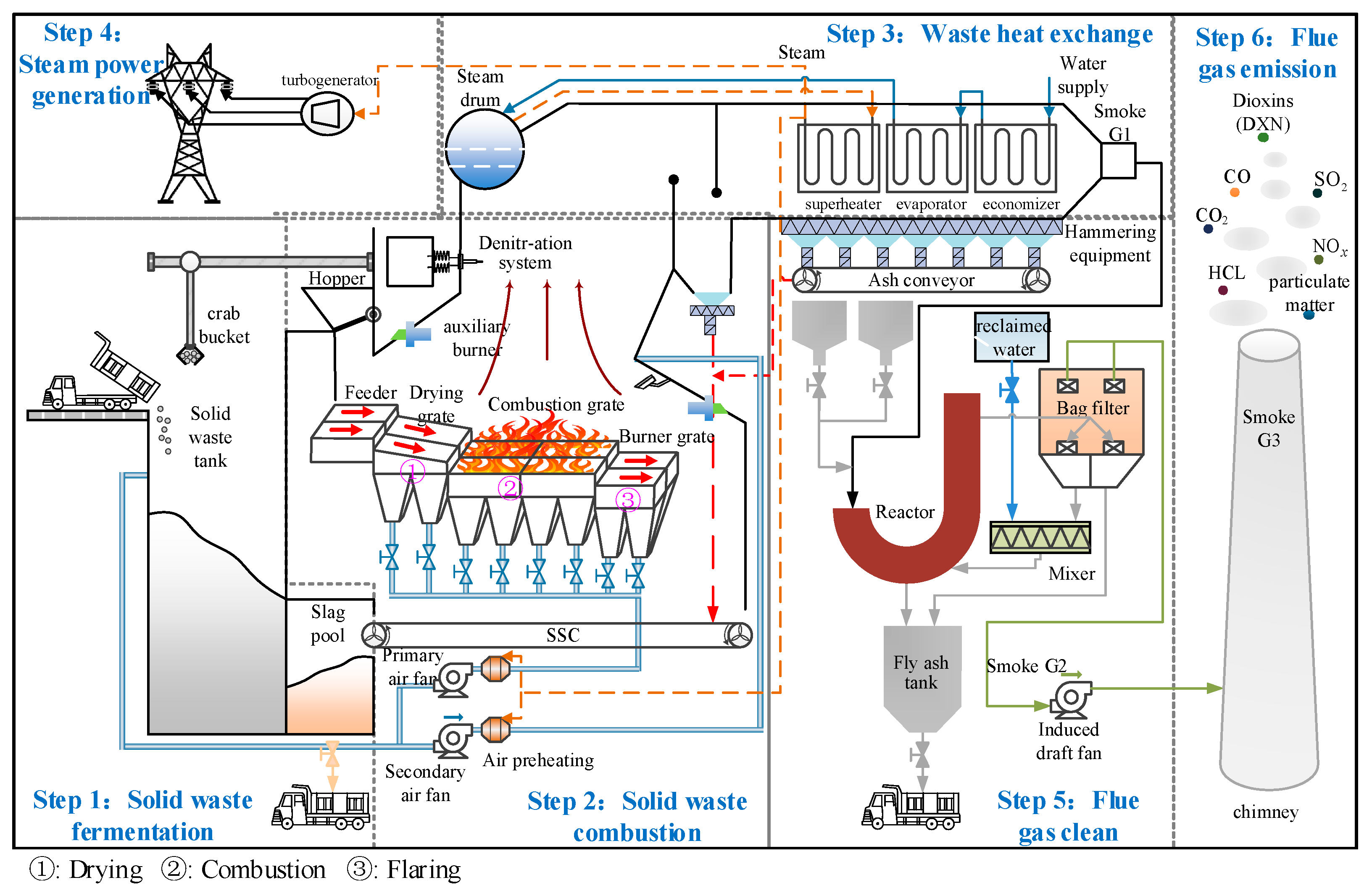
Figure 1. Process flow diagram of an actual MSWI power plant.
Applsci 15 10329 g001
Figure 2. Diagram of the SDHETM-IT2FB-ACMPC control strategy.
Applsci 15 10329 g002
Figure 3. Prediction curve. The proposed IT2FBLS model can fit the true values and is closer to the true values than other models.
Applsci 15 10329 g003
Figure 4. Prediction error curve. Compared with other models, the proposed IT2FBLS model has the smallest prediction error for most of the samples.
Applsci 15 10329 g004
Figure 5. FT control curves of each controller. The proposed method did not show significant fluctuations, and the enlarged graph indicates that it has the fastest convergence speed.
Applsci 15 10329 g005
Figure 6. FT control error curves of each controller. The magnification diagram shows that the proposed method is capable of keeping the absolute value of the control error at the minimum level for the vast majority of the time. It indicates that the proposed method has greater robustness.
Applsci 15 10329 g006
Figure 7. SV curve of SDHETM-IT2FB-ACMPC. The ACOC method effectively determines the optimal solution for the control variables at each triggering moment, and the proposed method can effectively control the FT.
Applsci 15 10329 g007
Figure 8. Objective function curve of SDHETM-IT2FB-ACMPC. Except when the set point changes, the proposed method always maintains the objective function value near 0. The stability of the controller has been verified.
Applsci 15 10329 g008
Figure 9. Trigger interval time of SDHETM-IT2FB-ACMPC. The proposed method only triggers denser intervals when the setpoint changes.
Applsci 15 10329 g009
Figure 10. Trigger times curve of SDHETM-IT2FB-ACMPC. The curve shows that the proposed method makes the triggering times about a quarter of the original.
Applsci 15 10329 g010
Table 1. Key process variable PCC value.
NumberVariablePCC Value
1PV0.0553
2SV0.2045
3FS0.0621
4DS0.0589
5AI−0.2947
Table 2. The actual ranges of process variables.
VariableUnitVariation Range
PVm3/h[53.78, 76.71]
SVm3/h[0, 20.88]
FS%[20, 53.75]
DS%[20, 60]
AIL/h[16.75, 84.42]
FT°C[922, 1066]
Table 3. Performance indicators of prediction models.
ModelMSERMSEMAER2
IT2FBLS1.1940 × 1013.4554 × 1002.5692 × 1009.6730 × 10−1
FBLS1.3331 × 1013.6512 × 1002.7148 × 1009.6349 × 10−1
IT2FNN [20]1.4990 × 1013.8717 × 1002.8950 × 1009.5895 × 10−1
FNN [41]1.5532 × 1013.9411 × 1003.0292 × 1009.5747 × 10−1
BPNN [11]1.9008 × 1014.1079 × 1003.2008 × 1009.5379 × 10−1
Note: The best model and results are highlighted in bold. For MSE, RMSE, and MAE, smaller values indicate the best performance. For R2, a larger value indicates the best performance.
Table 4. Comparison of performance indicators.
ControllerPerformance IndicatorTriggering Times
ISEIAEDEVmax
IT2FBLS-ACN-PID [42]0.46260.36169.87081200
NMPC [11]1.34560.47597.26671200
FNN-MPC [41]1.05810.39538.81601200
IT2FNN-MPC [20]0.79090.33387.34631200
LSTM-MPC [43]0.68850.34856.94861200
FBLS-MPC0.66950.34316.72021200
IT2FB-MPC0.28800.19476.62691200
I2T2FB-MPC [44]0.28720.19486.62691200
IT2FB-ACMPC0.28210.19306.62691200
SDHETM-IT2FB-MPC0.31740.20456.6269370
SDHETM-IT2FB-ACMPC0.30840.19696.6269343
Note: The best result and the controller with the best overall performance are highlighted in bold. Smaller values represent the best performance in each indicator.
Disclaimer/Publisher’s Note: The statements, opinions and data contained in all publications are solely those of the individual author(s) and contributor(s) and not of MDPI and/or the editor(s). MDPI and/or the editor(s) disclaim responsibility for any injury to people or property resulting from any ideas, methods, instructions or products referred to in the content.