Abstract
As oil and gas exploration extends to deep, ultra-deep, and unconventional reservoirs, high drilling costs persist. Drill bit performance, as the critical rock-breaking component, directly governs efficiency and economics. While optimal bit selection boosts rate of penetration (ROP) and cuts costs, traditional expert-dependent methods struggle to address complex formation bit parameter interactions, suffering from low accuracy and poor adaptability. With artificial intelligence gaining traction in petroleum engineering, machine learning-based bit selection has emerged as a key solution. This study focuses on polycrystalline diamond compact (PDC) bits and proposes an intelligent bit selection method based on graph neural networks (GNNs), utilizing drilling records from over 100 wells encompassing 40 multidimensional features. Through comparative analysis of four intelligent models—random forest, gradient boosting (XGBoost), gated recurrent unit (GRU), and the GNN, the results demonstrate that the GNN achieves superior performance with an R2 (coefficient of determination) of 0.932 and MAPE (mean absolute percentage error) of 6.88%. The GNN significantly outperforms conventional models in rock-breaking performance prediction. By establishing this GNN model for ROP and footage per run prediction, this study achieves intelligent bit selection that substantially enhances drilling efficiency, reduces operational costs, and provides scientifically reliable technical support for drilling operations in complex formation conditions.
1. Introduction
In oil and gas exploration and development, drilling is one of the most critical operational processes [1]. With the current trend of drilling operations shifting toward “two deeps and one unconventional” (deep, ultra-deep, and unconventional reservoirs) [2], drilling costs remain persistently high. The drill bit, as the core tool in drilling operations, directly impacts rate of penetration (ROP), wellbore quality, and operational costs. Therefore, selecting the optimal drill bit is crucial for improving drilling efficiency and reducing costs.
Currently, traditional drill bit selection methods mainly fall into three categories: performance evaluation methods, rock mechanics parameter methods, and comprehensive methods [3]. Performance evaluation methods rely heavily on historical experience and expert judgment, introducing significant subjectivity, including the gray clustering method [4] and the composite cost-per-meter formula. They struggle to quantify the dynamic matching relationship between bit performance and formation conditions. The rock mechanics parameter method, such as the acoustic travel time method [5], internal friction angle selection method [6], and confined rock compressive strength method [7,8], is based on theoretical models but exhibits poor adaptability in complex formations and often neglects factors such as bit wear and hydraulic parameters. Both approaches face challenges such as insufficient data utilization and poor formation compatibility, making it difficult to make rapid and accurate bit selection decisions under varying operating conditions, lithological changes, and formation complexities. In contrast, comprehensive methods integrate field data analysis with rock mechanics modeling, reducing subjective bias to some extent and establishing a more holistic evaluation system, thereby significantly improving decision reliability. However, in practice, these methods still encounter challenges such as high modeling complexity and large-scale data processing demands, necessitating the adoption of intelligent technologies to further enhance decision-making efficiency.
In recent years, multidimensional scoring systems have emerged as a critical methodology for drill bit selection, significantly enhancing drilling efficiency while optimizing operational costs, thereby overcoming the limitations of conventional single parameter decision-making approaches. Neamat Jameel et al. demonstrated this advancement through the simultaneous analysis of ROP versus cost per meter correlations, bit wear patterns, and formation compatibility, coupled with real time adjustments of weight on bit (WOB) and rotation speed parameters [9]. Their field applications in northern Iraq oilfields achieved remarkable efficiency improvements compared to traditional methods. Similarly, Bambang Yudho Suranta’s research team developed a comprehensive quantitative scoring system incorporating four key parameters: ROP, wear grading evaluation, cost per foot, and mechanical specific energy (MSE). Their systematic approach conclusively validated the superior performance of PDC bits in 12¼ inch quartzite formations for XYZ Company’s geothermal wells in Indonesia [10]. These case studies collectively demonstrate that multiparameter collaborative optimization has become the prevailing technical paradigm for modern drill bit selection.
Meanwhile, with the deep integration of digital technologies in the oil and gas industry [1], the intelligent trend in drill bit selection is becoming increasingly prominent. The intelligent bit selection method is based on artificial intelligence algorithms, such as the roller cone bit selection using feedforward neural networks by H. I. Bilgesu [11] and A. F. Al Rashidi [12]. Building upon this work, Zhao et al. developed an enhanced PCA-BP neural network approach that integrates backpropagation algorithms with principal component analysis to optimize bit selection processes [13]. Further progress was achieved by Yan et al., who implemented a trilayer BP neural network model through numerical simulation to quantitatively correlate PDC bit configuration parameters with formation drill ability indices, enabling customized bit series design for specific oilfield applications [14]. The methodology reached greater sophistication through Zhang et al.’s comprehensive formation drill ability evaluation system, which incorporated well logging interpretation data, laboratory core analysis results, and systematically encoded petromechanical parameters into neural network training datasets [15]. This integrated approach successfully established predictive relationships between formation characteristics and optimal bit types using BP neural networks, representing a significant advancement in data-driven drilling optimization. These consecutive innovations demonstrate the petroleum industry’s progressive adoption of machine learning techniques, evolving from initial algorithm development to practical field implementation and ultimately to comprehensive predictive systems that enhance drilling efficiency and performance.
Compared to traditional AI methods, graph neural networks (GNNs) offer superior capabilities in modeling the relationships between formation parameters and key bit characteristics. They demonstrate significant advantages in handling multi-dimensional, highly interconnected data involving formation properties, lithology, and bit features, thereby further improving the accuracy and generalization ability of intelligent bit selection.
2. Methodology
2.1. Model Construction
2.1.1. Random Forest
Random Forest, proposed by Breiman [16] and Cutler [17], is an ensemble learning algorithm that constructs multiple decision trees through bootstrap resampling and determines the final result via voting. This model exhibits advantages such as high accuracy, strong resistance to overfitting, and excellent capability in handling high-dimensional data, demonstrating outstanding performance in classification and regression tasks. Compared to a single decision tree, Random Forest can better capture nonlinear relationships between bit parameters and formation characteristics while reducing overfitting risks through random feature selection, making it particularly advantageous for bit optimization.
As shown in Figure 1, based on dataset characteristics, this study employs feature engineering and ensemble learning methods to construct a Random Forest model. During the feature processing stage, Recursive Feature Elimination (RFE) [18] was used to screen five key features from the initial 17 features, with a threshold of 0.4 applied to identify critical parameters. Dynamic weighting based on feature importance scores was implemented to effectively reduce model complexity and enhance feature discriminability. In the model construction phase, bootstrap sampling was adopted to build multiple decision trees, with each tree randomly selecting a subset of features. The optimal splitting points were determined by minimizing MSE, continuing until the preset depth was reached. The final prediction results were obtained by aggregating all decision trees, significantly improving model robustness. Additionally, the Mean Absolute Percentage Error (MAPE) was selected as the loss function to optimize the training process and enhance prediction accuracy.
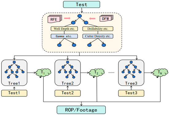
Figure 1.
Random forest model.
2.1.2. XGBoost
XGBoost (eXtreme Gradient Boosting) is a machine learning system based on boosted trees proposed by Chen [19] et al., building upon extensive prior research on gradient boosting algorithms. It comprises an ensemble of iteratively generated residual trees, where each tree learns the residuals from the previous N-1 trees. The final prediction for a sample is obtained by summing the output values of all individual trees [20]. In this model, each tree attempts to correct the prediction errors of its predecessors, and the final prediction result is derived from a weighted summation of all trees’ outputs [21]. Compared to traditional methods, XGBoost introduces improvements such as regularization, parallel computing, and second-order gradient optimization, supporting feature importance analysis. It exhibits high prediction accuracy, fast computational efficiency, and strong resistance to overfitting. Its unique gradient boosting mechanism makes it particularly suitable for processing structured data in bit optimization, demonstrating outstanding performance in both model accuracy and computational efficiency.
As shown in Figure 2, given the similarities between XGBoost and Random Forest models, this study similarly employs feature engineering and ensemble learning methods to construct an XGBoost prediction model. First, feature importance was dynamically evaluated based on feature gain, with a threshold of 0.4 applied to screen key features. A weighting mechanism was introduced to amplify the influence of important features. During model construction, XGBoost decision trees were iteratively generated, and the histogram algorithm was used to accelerate the feature splitting process. The optimal splitting points were determined by maximizing the objective function gain. The model adopted MSE as the loss function, combined with L1/L2 regularization terms to form the objective function. Through gradient boosting techniques, the model was progressively optimized, ensuring prediction accuracy while effectively controlling model complexity.
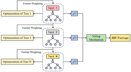
Figure 2.
XGBoost model.
2.1.3. Gated Recurrent Unit
The Gated Recurrent Unit (GRU) is another gated RNN unit introduced by Cho [22] et al. in the context of machine translation, effectively addressing the vanishing gradient problem of traditional RNNs in long-sequence modeling. Compared to LSTM, the GRU model is renowned for its capability in processing time-series data [23]. While maintaining comparable performance, it features a more streamlined network architecture, higher training efficiency, and greater suitability for real-time application scenarios. In drilling engineering applications, GRU demonstrates superior capability in processing time-series features such as Measurement While Drilling (MWD) data and drilling parameters, effectively capturing their dynamic variation patterns and long-term dependencies. Moreover, its gating mechanism enables adaptive selection of critical information for propagation while filtering out noise interference, thereby providing more accurate time-series feature analysis for optimized bit selection.
Given that the dataset contains both static parameters (e.g., bit structural features) and dynamic parameters generated during drilling operations, as shown in Figure 3, this study developed a hybrid model based on the GRU temporal architecture to better integrate structural and temporal characteristics. The proposed architecture consists of four key modules: structural feature unit, temporal feature unit, feature fusion with GRU processing module, and prediction layer. The structural feature network employs a dual fully connected layer configuration with batch normalization, the rectified linear unit (ReLU) activation, and Dropout (rate = 0.3) to process static bit parameters. The temporal feature network utilizes 1D convolution combined with batch normalization, ReLU activation, and max pooling to extract dynamic parameter features. The feature fusion module concatenates these two feature types before feeding them into dual GRU layers for temporal modeling. Finally, the prediction layer is used to achieve the prediction of two key rock-breaking performance indicators: ROP and footage per run. The model adopts MSE as the optimization objective to effectively combine the advantages of feature extraction and time-series modeling.
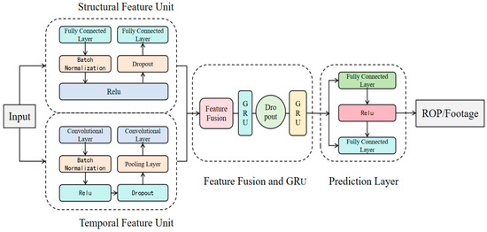
Figure 3.
GRU model.
2.1.4. Graph Neural Network
Graph Neural Networks (GNNs) are a deep learning methodology. Research on graph neural network seeks to generalize the convolutional neural network to a graph representation [24]. With their powerful representational capabilities, GNNs have emerged as a widely adopted approach for graph analysis. Unlike traditional neural networks that can only process structured (Euclidean) data, a GNN iteratively updates its vertex features by aggregating features along the edges [25]. Graph Neural Networks, with their flexible representation learning framework, offer a promising solution to the fundamental limitation of traditional deep learning methods in effectively modeling and reasoning about relational data [26].
In GNNs, a graph is typically represented as , consisting of nodes and edges. Here, denotes the node set where each node possesses a feature vector representing a data entity, while represents the edge set indicating connections between nodes, with each edge describing the relationship between nodes and [27]. By capturing relationships between nodes and their neighbors, GNNs can learn representations of nodes, edges, and entire graphs, demonstrating unique advantages in processing non-Euclidean data. This approach has been widely applied in fields such as social networks, molecular structures, knowledge graphs, and recommendation systems.
Based on feature selection results, this study utilizes geomechanical parameters, engineering data, and bit parameters as node features, while establishing inter-node connections through multiple methods including cosine similarity. By integrating convolutional neural network technology, we constructed a Graph Convolutional Network (GCN) prediction model. The model architecture comprises three components (as shown in Figure 4): the graph convolutional network module, global average pooling layer module, and predictor module. The specific construction methods for each module are as follows:
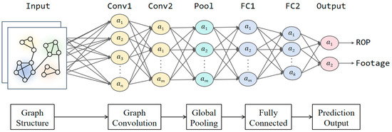
Figure 4.
GNN model.
- Graph Convolutional Network Module
The graph convolutional network module consists of two GCN layers designed to progressively extract and aggregate feature information from the graph structure. The input dimension of the first GCN layer is determined by the data features, with an output dimension of 64 (i.e., the hidden layer dimension). Through graph convolution operations, this layer transforms the input features into hidden layer representations, effectively capturing local structural information between nodes and their neighbors. The output undergoes batch normalization to accelerate model convergence and stabilize the training process, while the ReLU activation function introduces nonlinearity to enhance the model’s representational capacity. Additionally, to prevent overfitting, a dropout layer with a rate of 0.3 is applied for regularization, randomly deactivating a portion of neurons during training. The second GCN layer maintains input and output dimensions of 64, performing further graph convolution operations on the first layer’s output to extract higher-level graph structural information. Similarly to the first layer, its output is processed with batch normalization to maintain feature distribution stability and ReLU activation to strengthen nonlinear expressiveness.
- 2.
- Global Average Pooling Module
Following the second GCN layer, the model employs global average pooling to aggregate node features into a global feature vector. Both the input and output dimensions of this layer are 64. The pooling operation generates a fixed-length global representation that effectively reflects the overall graph characteristics, providing a unified input for subsequent prediction tasks.
- 3.
- Predictor Module
The predictor module comprises two fully connected (FC) layers, ReLU activation, and dropout regularization, mapping the globally pooled feature vector to the final prediction output. The first FC layer reduces the feature dimension from 64 to 32 through linear transformation, extracting higher-level feature representation.
2.2. Evaluation Metrics
2.2.1. Mean Absolute Percentage Error
MAPE was selected as the evaluation metric for each model, used to measure the relative error percentage between the predicted values and the true values [28], where represents the number of sample points, represents the rate of penetration, and represents the predicted rate of penetration.
2.2.2. R-Squared
R2 serves as another evaluation metric, used to measure the model’s ability to explain the variance of the target variable [29], where represents the actual observed value of the sample, represents the predicted value of the corresponding sample, is the arithmetic mean of all actual values, and is the total sample size.
2.3. Model Optimization
2.3.1. Hyperparameter Search with Cross-Validation
Hyperparameter search with cross-validation is a systematic machine learning model optimization method that determines the optimal parameter configuration by combining parameter search strategies with cross-validation techniques [30]. In this study, we applied hyperparameter search with cross-validation to optimize both Random Forest and XGBoost models. First, we constructed a multidimensional search space for key parameters in the machine learning models, including the number of trees, maximum depth, and learning rate. We then performed an exhaustive evaluation of all possible parameter combinations through parameter search. During the evaluation process, we adopted a 5-fold cross-validation strategy, where the original dataset was randomly but uniformly divided into five complementary subsets, followed by five rounds of training-validation cyclic testing to ensure each data point participated in validation. Additionally, we preset a fixed random seed to guarantee the reproducibility of experiments. This optimization method, through comprehensive exploration of the parameter space and rigorous validation procedures, ultimately identified the hyperparameter combination that demonstrated optimal performance in cross-validation, thereby significantly improving the model’s predictive performance and generalization capability. The optimal parameter combinations for Random Forest are shown in Table 1, while those for XGBoost are presented in Table 2.

Table 1.
Optimal parameter combination for random forest model.
Table 2.
Optimal parameter combination for XGBoost.
2.3.2. Adam Optimizer
The Adam optimizer (Adaptive Moment Estimation) is an adaptive learning rate optimization algorithm that combines the advantages of momentum gradient descent and RMSProp algorithms [31]. In this study, the Adam optimizer was employed to optimize the GRU model. The implementation process was as follows: First, the training data was loaded using random shuffling. Then, the model was trained utilizing the adaptive learning rate characteristic and weight decay mechanism of the Adam optimizer, with an initial learning rate set to 0.01 and weight decay value set to 0.01, effectively controlling model complexity and preventing overfitting. Building upon this foundation, the ReduceLROnPlateau [32] learning rate scheduler was introduced to dynamically adjust the learning rate based on validation loss. When the validation loss showed no improvement over five consecutive training epochs, the learning rate was reduced by a factor of 0.5, thereby accelerating convergence and avoiding local optima.
2.3.3. AdamW Optimizer
AdamW is an improved version of the Adam optimizer that effectively enhances model generalization capability by decoupling L2 regularization from weight decay [33]. This optimizer utilizes first-order moment (momentum) and second-order moment (adaptive learning rate) estimates of gradients, combined with a bias correction mechanism, to dynamically adjust learning rates for each parameter. In this study, the specific parameter settings were as follows: learning rate 0.005, weight decay 1 × 10⁻⁴. These settings ensured model convergence speed while avoiding training instability caused by excessive learning rates.
3. Case Results
3.1. Multi-Source Data Fusion
3.1.1. Dataset Description
The study utilizes a comprehensive database integrating geomechanical parameters, engineering data, and key bit characteristic parameters. For each well, data were extracted according to bit models, with each PDC bit model corresponding to a dataset comprising geomechanical properties, engineering parameters (including footage per run, pure drilling time, and ROP), and bit design features. The original dataset comprises 560 drilling records from 68 wells, with each record containing 40 characteristic parameters. It should be noted that these 560 records are actually derived from dimensionality reduction in multiple bit-run records. Specifically, we used the averaged geomechanical parameters for each well section to simplify the representation of geological variations within that interval. However, preliminary analysis revealed a data missing rate of nearly 60% due to challenges such as complex field data acquisition conditions, equipment failures, and manual recording omissions, necessitating rigorous data cleaning to obtain a high-quality dataset.
3.1.2. Data Cleaning
Given the dataset characteristics, this study first employed two common outlier detection methods—boxplot analysis [34] and standard deviation filtering—to identify and remove anomalies. To address the substantial missing data issue, a tiered imputation strategy was implemented based on data types. For geomechanical parameters, missing values were reconstructed through petrophysical calculations derived from existing well-logging data. Drill bit attribute gaps were populated by matching bit models against an established bit characteristic database. Subsequently, missing values were supplemented through similarity-based imputation using offset well data from adjacent boreholes. These domain-informed methods collectively reduced the overall missing rate to approximately 10%.
Building upon these imputation results, for numerical continuous features (e.g., WOB, acoustic transit time, unconfined compressive strength), median imputation was applied for missing value filling. For categorical discrete features (e.g., formation type, lithology, number of blades), a most frequent value imputation strategy was adopted. Finally, one-hot encoding was used to process textual information in the dataset. Through this systematic data cleaning workflow, a refined dataset of 355 high-quality records from 60 wells was obtained. Figure 5 presents a comparison of data cleaning results, using WOB as an example.
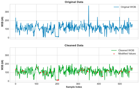
Figure 5.
Comparison of data cleaning results.
3.1.3. Feature Selection
This study applied Pearson correlation coefficient analysis [34] to evaluate the linear correlation between independent variables and target parameters. Based on the statistical significance level of correlation metrics and domain expertise, 17 highly relevant features were selected (Table 3), forming the optimal feature set for subsequent modeling.
Table 3.
Preferred characteristics.
3.2. Model Performance Comparison
Under the optimized model parameters, we employed the developed models to predict two key rock-breaking performance indicators—ROP and footage per run—for Well JY107-S1HF in the Fuling Shale Gas Hongxing Block. To provide a comprehensive evaluation of bit performance, we integrated these two parameters into a composite index, as presented in Figure 6.
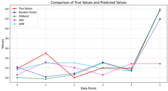
Figure 6.
Comparison of model prediction.
As shown in Figure 7, based on the comparative analysis of model performance data, the GNN demonstrates significant advantages in bit selection tasks. In terms of prediction accuracy, the GNN model achieves an R2 score of 0.974 for ROP prediction, representing improvements of 5.9%, 40.9%, and 936% compared to Random Forest (0.919), XGBoost (0.691), and GRU (0.094), respectively; for footage per run prediction, GNN’s R2 score of 0.890 shows improvements of 14.7% and 18% over Random Forest (0.776) and XGBoost (0.754); in the Comprehensive Performance Index (CPI), GNN’s R2 score of 0.932 indicates improvements of 9.9% and 28.9% over Random Forest (0.848) and XGBoost (0.723). As shown in Figure 8, regarding error control, the GNN model achieves a MAPE of 4.09% for ROP prediction, with reductions of 52.6%, 75.8%, and 85.8% compared to Random Forest (8.63%), XGBoost (16.89%), and GRU (28.72%); for footage per run prediction, GNN’s MAPE of 9.67% shows reductions of 11%, 14.3%, and 51.1% compared to Random Forest (10.86%), XGBoost (11.28%), and GRU (19.77%); in CPI, GNN’s MAPE of 6.88% demonstrates reductions of 29.4%, 51.2%, and 71.6% compared to Random Forest (9.75%), XGBoost (14.09%), and GRU (24.25%)
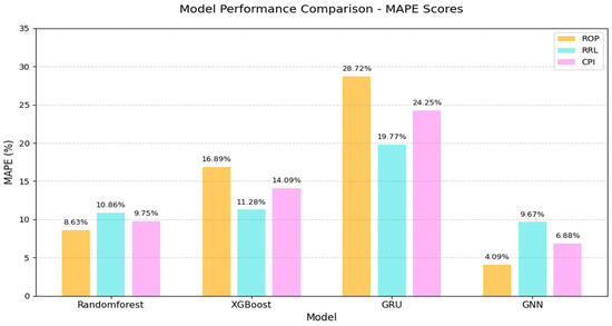
Figure 7.
Model performance comparison-MAPE scores.
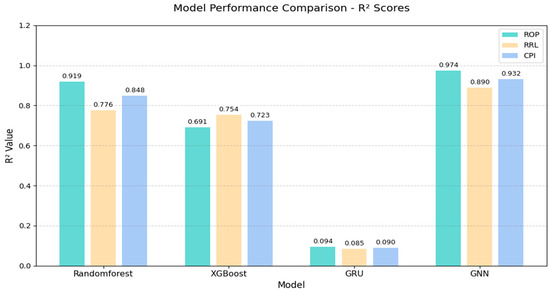
Figure 8.
Model performance comparison-R2 scores.
3.3. Bit Optimization
3.3.1. Rock-Breaking Mechanism of PDC Bits
The PDC bit is an indispensable high-efficiency rock-cutting tool in modern drilling operations. Its superior drilling performance primarily depends on the optimized configuration of multiple key characteristic parameters. As core elements in bit selection, as shown in Figure 9, the rational combination of critical parameters such as cutter size, back rake angle, cutter density, bit diameter, and blade configuration not only directly affect the bit’s rock-breaking efficiency and service life but also determines the overall drilling stability and economic performance. Scientific matching and optimized design of these parameters based on target formation lithology characteristics and actual engineering requirements can significantly enhance the bit’s formation adaptability and ROP, while reducing drilling vibration risks, thereby providing reliable assurance for efficient drilling operations.
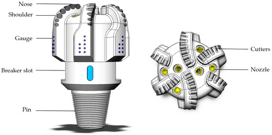
Figure 9.
Structure diagram of PDC bit.
3.3.2. Offset Well Data Construction
This study systematically analyzes key logging parameters including acoustic transit time, gamma ray values, and unconfined compressive strength from multi-source data of offset wells in the target block. By integrating real-time mud logging data such as WOB and rotary speed with operational performance metrics including historical bit’s rate of penetration and footage per run, we methodically screen logging and mud logging parameters that match the target well section, which serve as the basis for optimal bit selection in the target interval.
3.3.3. Bit Feature Population Construction
To establish a diversified range of bit parameter combinations, this study identified seven key characteristics that most significantly impact drilling performance from the bit feature database, based on field experience and design priority sequence. These critical parameters include bit aggressiveness, primary cutter diameter, cutter density, and number of blades. Through statistical analysis of historical design iterations and drilling trip data, we evaluated the occurrence frequency of each parameter in the target well section to determine optimal bit selection. This methodology ultimately screened 30 distinct bit feature combinations—representing 30 potential bit models suitable for this specific well section—thereby constructing a comprehensive bit characteristic population.
3.3.4. Bit Optimization Results
As shown in Figure 10, based on the constructed offset well data and bit feature population, these were input into the model to predict the ROP and footage per run for different bit feature combinations in each section of the planned well. The predictions were integrated into a composite index serving as the predictive score for each feature combination, which were then ranked and screened to obtain the top-performing bit feature combinations for each well section. The selected combinations were then matched against 74 distinct drill bit types from the bit characteristic database, ultimately identifying the optimal bit models for each section of the planned well.
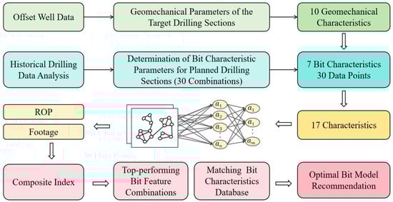
Figure 10.
Flowchart of PDC bit optimization method.
The drill bit optimization results for each section of Well JY107-S1HF are presented in Table 4. A comparison of the ROP before and after bit optimization is shown in Figure 11. It can be observed that the optimized bit types significantly improved drilling efficiency in all sections.
Table 4.
Drill bit optimization results.
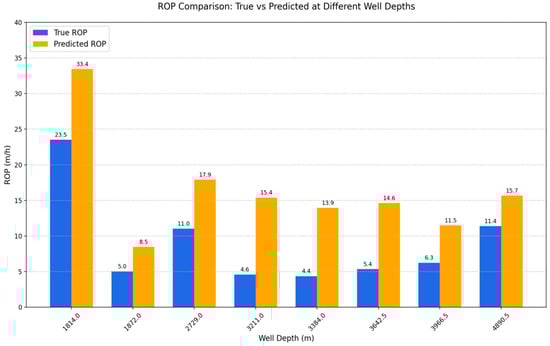
Figure 11.
Comparison of the ROP before and after bit optimization.
In the shallow section (1814 m), the ROP increased from 23.51 m/h to 33.43 m/h, a 42.2% improvement, demonstrating the superior rock-breaking performance of the optimized bit in softer formations. In the 1872 m section, the ROP increased from 5.03 m/h to 8.46 m/h, a 68.2% improvement, confirming the stable performance enhancement of bit optimization in shallow-to-intermediate formations. For the mid-deep section (2729 m), the ROP improved from 11.03 m/h to 17.90 m/h, a 62.3% increase, indicating excellent adaptability of the optimized bit to mid-deep formations. In the deepest section (4890.5 m), the ROP increased from 11.38 m/h to 15.66 m/h, a 37.6% improvement, suggesting that the bit optimization strategy still delivered performance gains even in hard, deep formations.
4. Discussion
The above research results indicate that, from the perspectives of model architecture and algorithmic characteristics, there are significant performance differences among random forest, XGBoost, GRU, and GNN models in predicting bit rock-breaking performance.
Benefiting from its ensemble learning mechanism and internal structure, random forest reduces the risk of overfitting in individual decision trees by constructing multiple trees and integrating their outputs. Through random feature selection and data sampling, it enhances model generalization. However, compared to GNNs, this mechanism still shows limitations. XGBoost, with its gradient boosting algorithm, iteratively minimizes prediction errors, yet its performance suffers when handling high-noise, low-correlation data due to sensitivity to outliers. GRU, as a variant of recurrent neural networks, excels in processing time-series data. However, in this drilling dataset, temporal features are not prominent, and GRU’s ability to extract non-temporal features is relatively weak, resulting in the poorest performance.
In contrast to traditional machine learning models, GNNs demonstrate three core advantages in handling non-Euclidean data for bit optimization: topological structure modeling capability, dynamic relationship learning ability, and multi-source feature fusion capability.
First, in terms of topological structure modeling, GNNs overcome the limitation of traditional methods that treat data as independent and identically distributed samples. By constructing a graph structure incorporating bit parameters, formation characteristics, and operational conditions, GNNs explicitly represent topological connections among these elements, establishing a comprehensive and physically interpretable representation system. This modeling approach is particularly suitable for describing the complex interaction networks among multiple factors in drilling processes.
Second, GNNs possess a dynamic relationship learning ability through an innovative message-passing mechanism. In each graph convolutional layer, node features are dynamically updated based on their neighboring nodes’ states, enabling information propagation over multiple hops. In bit optimization, this advantage allows the model to automatically learn the mapping relationship between “specific formation conditions → optimal bit parameters” and the mutual influences between different well sections, thereby improving prediction accuracy.
Lastly, GNNs exhibit superior multi-source feature fusion capability, enabling the integration of heterogeneous data. In practical applications, the model can simultaneously process multi-dimensional features, including bit design parameters (e.g., cutter density, blade count), drilling operation data (e.g., acoustic travel time, gamma ray), and formation properties (e.g., compressive strength, lithology). By designing different feature aggregation strategies, GNNs not only facilitate the joint analysis of static and dynamic parameters but also balance local characteristics with global optimization. This multi-scale, multi-source data fusion capability allows the model to comprehensively evaluate the impact of various factors on bit performance, leading to more scientific and reliable optimization decisions.
Therefore, the research findings demonstrate that adopting GNNs for bit optimization not only significantly enhances prediction accuracy and generalization ability but also provides a new intelligent solution for drilling engineering, paving the way for data-driven decision-making in complex downhole environments. However, it should be noted that this study evaluated the performance of optimized drill bits by predicting the rate of penetration and bit footage based on predetermined geomechanical parameters of target wells, rather than through actual field trials. This methodological approach inevitably carries certain limitations regarding practical validation.
5. Conclusions
This study first established standardized cleaning and integration procedures for bit parameters, logging data, and mud logging data, resulting in a high-quality dataset comprising 355 records from 60 wells, from which 17 key characteristic parameters for bit optimization were selected. Research demonstrates that this multi-source data fusion approach effectively combines static bit characteristic parameters (such as cutter density and back rake angle), drilling parameters (including WOB and rotary speed), and formation characteristic parameters (like acoustic transit time and unconfined compressive strength), overcoming the limitations of traditional methods that rely on single data sources and incomplete information, thereby enhancing the reliability of final optimization results.
Secondly, the study developed four rock-breaking performance prediction models incorporating Random Forest, XGBoost, GRU, and GNN, systematically evaluating each model’s performance in predicting bit rock-breaking efficiency. Experimental results show that the GNN, through its graph structure learning mechanism, excels in modeling complex nonlinear relationships between bit parameters and formation characteristics, achieving an R2 of 0.932 and MAPE of 6.88%, demonstrating significant performance advantages over Random Forest, XGBoost, and GRU. The research confirms that GNNs provide substantial technical advantages for bit optimization tasks, offering a novel solution for intelligent drilling engineering.
Finally, based on the GNN model, the study predicted the ROP and footage per run for constructed offset well data and bit feature populations in planned wells, ultimately selecting the optimal bit models from 74 available types from the bit characteristic database for target well sections. The findings reveal that GNN-based bit optimization delivers significant improvements in drilling speed, validating the method’s reliability in practical applications and providing a scientific foundation for bit selection in drilling operations.
Author Contributions
Conceptualization, N.L. and C.Z.; methodology, N.L.; software, T.X.; validation, N.L., C.Z. and Z.Z.; formal analysis, S.Y.; investigation, L.C.; resources, Z.Z.; data curation, C.W.; writing—original draft preparation, M.H. and N.L.; writing—review and editing, C.Z.; visualization, T.X. and X.L.; supervision, C.Z.; project administration, N.L.; funding acquisition, C.Z. All authors have read and agreed to the published version of the manuscript.
Funding
This research received no external funding.
Data Availability Statement
The original contributions presented in this study are included in the article. Further inquiries can be directed to the corresponding author.
Conflicts of Interest
Authors Ning Li, Tianguo Xia, and Long Chen were employed by the company PetroChina Tarim Oilfield Company. The remaining authors declare that the research was conducted in the absence of any commercial or financial relationships that could be construed as a potential conflict of interest.
References
- Li, G.; Song, X.; Zhu, Z.; Tian, S.; Sheng, M. Research progress and the prospect of intelligent drilling and completion technologies. Pet. Drill. Technol. 2023, 51, 35–47. [Google Scholar]
- Li, M.; Liu, C.; Liu, S.; Shen, B.; Zhang, Y.; Guo, X. Theoretical and technological progress, challenges, and development directions of oil and gas exploration of Sinopec during the 14th Five-Year Plan period. China Pet. Explor. 2025, 30, 1–14. [Google Scholar] [CrossRef]
- Kun, Z. Research on Bit Selection Methods for Target Formations. Pet. Chem. Constr. 2022, 44, 159–162. [Google Scholar] [CrossRef]
- Wang, Y. The grey clustering method is used to evaluate bit types. Oil Drill. Prod. Technol. 1991, 13, 19–24. [Google Scholar] [CrossRef][Green Version]
- Bond, D. The optimization of PDC bit selection using sonic velocity profiles present in the Timor Sea. SPE Drill. Complet. 1990, 5, 135–142. [Google Scholar]
- Spaar, J.; Ledgerwood, L.; Goodman, H.; Graff, R.; Moo, T. Formation compressive strength estimates for predicting drillability and PDC bit selection. In Proceedings of the SPE/IADC Drilling Conference and Exhibition, Amsterdam, The Netherlands, 28 February 1995; p. SPE-29397-MS. [Google Scholar]
- Cordy, L.; Rogers, D.; Karsten, D.; Davies, R. Cumulative rock strength as a quantitative means of evaluating drill bit selection and emerging PCD cutter technology. In Proceedings of the IADC/SPE Asia Pacific Drilling Technology Conference and Exhibition, Jakarta, Indonesia, 9 September 2002; p. SPE-77217-MS. [Google Scholar]
- Fabian, R.; Birch, R. Canadian Application of PDC Bits Using Confined Compressive Strength Analysis. In Proceedings of the CADE/CAODC Spring Drilling Conference—April, Calgary, AB, Canada, 3–5 April 1995; pp. 19–21. [Google Scholar]
- Jameel, N.; Altaher, A.-H.Z.; Sarhad, M.; Kamal, Z.; Mohammed, B. Performance-Driven Drill Bit Selection Based on Field Investigations: Reducing Drilling Costs in Northern Iraq. Results Eng. 2025, 27, 106163. [Google Scholar] [CrossRef]
- Suranta, B.Y.; Sofyan, A.; Khoiriarta, F.; Handaja, S. Selection of Drilling Bit for the 12? Holes in the Geothermal Wells at the Company of XYZ. Int. J. Renew. Energy Res. 2024, 14, 701–710. [Google Scholar] [CrossRef]
- Bilgesu, H.; Al-Rashidi, A.; Aminian, K.; Ameri, S. A new approach for drill bit selection. In Proceedings of the SPE Eastern Regional Meeting, Wheeling, WV, USA, 17–19 October 2000; p. SPE-65618-MS. [Google Scholar]
- Rabia, H.; Farrelly, M.; Barr, M. A new approach to drill bit selection. In Proceedings of the SPE Europec featured at EAGE Conference and Exhibition, London, UK, 3–6 June 1986; p. SPE-15894-MS. [Google Scholar]
- Zhao, T.; Zhao, C.; Zhou, W.; Feng, X. Bit Optimization Method and Application Based on PCA-BP. Fault Block Oil Gas Field 2016, 23, 5. [Google Scholar]
- Jikun, Y. BP Neural Network-Based Optimization of PDC Bit Selection; China University of Petroleum (East China): Qingdao, China, 2017. [Google Scholar]
- Zhang, H.; Jiang, C.; Xiong, T.; Fan, G. Bit selection method based on BP neural network and rock drillability characteristics. Drill. Prod. Technol. 2019, 42, 4. [Google Scholar]
- Breiman, L. Random forests. Mach. Learn. 2001, 45, 5–32. [Google Scholar] [CrossRef]
- Cutler, A.; Cutler, D.R.; Stevens, J.R. Random forests. In Ensemble Machine Learning; Zhang, C.E., Ed.; Springer: New York, NY, USA, 2012; pp. 157–175. [Google Scholar]
- Granitto, P.M.; Furlanello, C.; Biasioli, F.; Gasperi, F. Recursive feature elimination with random forest for PTR-MS analysis of agroindustrial products. Chemom. Intell. Lab. Syst. 2006, 83, 83–90. [Google Scholar] [CrossRef]
- Chen, T.; Guestrin, C. Xgboost: A scalable tree boosting system. In Proceedings of the 22nd ACM SIGKDD International Conference on Knowledge Discovery and Data Mining, San Francisco, CA, USA, 13–17 August 2016; pp. 785–794. [Google Scholar]
- Friedman, J.; Hastie, T.; Tibshirani, R. Special invited paper. additive logistic regression: A statistical view of boosting. Ann. Stat. 2000, 28, 337–374. [Google Scholar] [CrossRef]
- Li, Z.; Liu, Z. Feature selection algorithm based on XGBoost. J. Commun. 2019, 40, 101–108. [Google Scholar]
- Cho, K.; Van Merriënboer, B.; Gulcehre, C.; Bahdanau, D.; Bougares, F.; Schwenk, H.; Bengio, Y. Learning phrase representations using RNN encoder-decoder for statistical machine translation. arXiv 2014, arXiv:1406.1078. [Google Scholar] [CrossRef]
- Hasanat, S.M.; Ullah, K.; Yousaf, H.; Munir, K.; Abid, S.; Bokhari, S.A.S.; Aziz, M.M.; Naqvi, S.F.M.; Ullah, Z. Enhancing short-term load forecasting with a CNN-GRU hybrid model: A comparative analysis. IEEE Access 2024, 12, 184132–184141. [Google Scholar] [CrossRef]
- Wu, Z.; Pan, S.; Chen, F.; Long, G.; Zhang, C.; Yu, P.S. A comprehensive survey on graph neural networks. IEEE Trans. Neural Netw. Learn. Syst. 2020, 32, 4–24. [Google Scholar] [CrossRef] [PubMed]
- Shi, W.; Rajkumar, R. Point-gnn: Graph neural network for 3d object detection in a point cloud. In Proceedings of the IEEE/CVF Conference on Computer Vision and Pattern Recognition, Seattle, WA, USA, 13–19 June 2020; pp. 1711–1719. [Google Scholar]
- Wu, T.; Cao, X.; Xian, X.; Yuan, L.; Zhang, S.; Tian, K. Advances of Adversarial Attacks and Robustness Evaluation for Graph Neural Networks. J. Front. Comput. Sci. Technol. 2024, 18, 1935–1959. [Google Scholar] [CrossRef]
- Wu, B.; Liang, X.; Zhang, S.; Xu, R. Frontier Advances and Applications of Graph Neural Networks. Chin. J. Comput. 2022, 45, 35–68. [Google Scholar]
- Myttenaere, A.D.; Golden, B.; Grand, B.L.; Rossi, F. Using the Mean Absolute Percentage Error for Regression Models. arXiv 2015, arXiv:1506.04176. [Google Scholar] [CrossRef]
- Cameron, A.; Windmeijer, F. An R-squared measure of goodness of fit for some common nonlinear regression models. J. Econom. 1997, 77, 329–342. [Google Scholar] [CrossRef]
- Soper, D.S. Greed is good: Rapid hyperparameter optimization and model selection using greedy k-fold cross validation. Electronics 2021, 10, 1973. [Google Scholar] [CrossRef]
- Kingma, D.; Ba, J. Adam: A Method for Stochastic Optimization. arXiv 2014, arXiv:1412.6980. [Google Scholar] [CrossRef]
- Sima, Z.; Tao, J.; Liu, Z. Adaptive and generic improvements to ResNet Backbone in image classification. In Proceedings of the International Conference on Electronics, Electrical and Information Engineering (ICEEIE 2024), Bangkok, Thailand, 10–12 May 2024; pp. 982–989. [Google Scholar]
- Llugsi, R.; El Yacoubi, S.; Fontaine, A.; Lupera, P. Comparison between Adam, AdaMax and Adam W optimizers to implement a Weather Forecast based on Neural Networks for the Andean city of Quito. In Proceedings of the 2021 IEEE Fifth Ecuador Technical Chapters Meeting (ETCM), Cuenca, Ecuador, 12–15 October 2021; pp. 1–6. [Google Scholar]
- Schwertman, N.C.; Owens, M.A.; Adnan, R. A simple more general boxplot method for identifying outliers. Comput. Stat. Data Anal. 2004, 47, 165–174. [Google Scholar] [CrossRef]


Disclaimer/Publisher’s Note: The statements, opinions and data contained in all publications are solely those of the individual author(s) and contributor(s) and not of MDPI and/or the editor(s). MDPI and/or the editor(s) disclaim responsibility for any injury to people or property resulting from any ideas, methods, instructions or products referred to in the content. |
© 2025 by the authors. Licensee MDPI, Basel, Switzerland. This article is an open access article distributed under the terms and conditions of the Creative Commons Attribution (CC BY) license (https://creativecommons.org/licenses/by/4.0/).