Abstract
In this study, the Binary Puma Optimizer (BPO) is introduced as a novel binary metaheuristic. The BPO employs eight Transfer Functions (TFs), consisting of four S-shaped and four V-shaped mappings, to convert the continuous search space of the original Puma Optimizer into binary form. To evaluate its effectiveness, BPO is applied to two well-known combinatorial optimization problems: the 0-1 Knapsack Problems (KPs) and the Uncapacitated Facility Location Problem (UFLP). The solver tailored for KPs is referred to as BPO1, while the solver for the UFLP is denoted as BPO2. In the UFLP experiments, only TFs are integrated into the solutions. Conversely, in the 0-1 KPs experiment, the additional mechanisms are (i) greedy-based population strategies; (ii) a crossover operator; (iii) a penalty algorithm; (iv) a repair algorithm; and (v) an improvement algorithm. Unlike KPs, the UFLP has no infeasible solutions, as facilities are assumed to be uncapacitated. Unlike KPs, the UFLP has no capacity constraints, as facilities are assumed to be uncapacitated. Thus, violations cannot occur, making improvement strategies unnecessary, and the BPO2 depends solely on TFs for binary adaptation. The proposed algorithms are compared with binary optimization algorithms from the literature. The experimental framework demonstrates the versatility and effectiveness of BPO1 and BPO2 in addressing different classes of binary optimization problems.
1. Introduction
Evolutionary algorithms have long been a model of innovation in computational problem-solving, drawing inspiration from natural processes and the behavior of primitive agents. These algorithms have been demonstrated to be effective instruments for addressing intricate optimization challenges, as they are driven by the inherent need to adapt and evolve [1]. In recent years, metaheuristic algorithms have been proposed as solutions to various challenges across multiple disciplines. The complexity of real-world applications is increasing. Operations research, robotics, machine learning, bioinformatics, and decision-making are among the primary areas of emphasis. Within the broader context of combinatorial optimization, binary optimization occupies a significant position. Consequently, researchers have initiated a series of scholarly investigations to transition algorithms from continuous optimization to binary optimization. Logic gates, Transfer Function (TF), and similarity measurement techniques are frequently employed in these adaptations to produce potential solutions. Specific techniques for measuring similarity have been implemented [2]. Conversely, adaptation methods such as TFs, angle modulation, or mod-based functions are required to convert algorithms designed for continuous values into binary-compatible formats [3]. Binary optimization frameworks are enhanced by integrating mechanisms such as Hill Climbing, crossover operation, greedy strategies, and XOR-based transformations to balance exploration and exploitation. Together, these methods enhance diversity, solution quality, and convergence, resulting in more robust and accurate performance across various problem domains [4].
Among recent metaheuristic algorithms, the Puma Optimizer (PO) has been introduced as a novel algorithm. Inspired by the life patterns and intelligent behaviors of pumas, PO was proposed as a novel approach. It included specific mechanisms for exploration and exploitation [5]. This study introduces the Binary Puma Optimizer (BPO), a novel binary metaheuristic algorithm designed to enhance the efficiency and effectiveness of binary optimization. The main contributions of this work can be summarized as follows:
- A novel binary metaheuristic, the BPO, is proposed as a binary adaptation of the original PO. Eight TFs, including four S-shaped and four V-shaped mappings, are systematically integrated into BPO to enable the transformation of continuous search dynamics into binary space.
- The two proposed variants, BPO1 and BPO2, are specifically designed to address different binary optimization problems. In particular, BPO1 incorporates several distinct mechanisms are designed to enhance its performance. The key features of these variants are outlined as follows:
- ○
- BPO1, designed to solve 0-1 KPs, incorporates additional mechanisms that ensure the total weight does not exceed the knapsack capacity, that infeasible solutions are corrected, and that feasible solutions are further improved to achieve higher profits. BPO1 incorporates the following additional mechanisms:
- (i)
- Greedy-based population strategies to generate diverse and high-quality initial solutions;
- (ii)
- Crossover operator to exchange information between parent and candidate solutions and preserve population diversity;
- (iii)
- Penalty Algorithm (PA) to address infeasible solutions;
- (iv)
- Repair Algorithm (RA) to restore feasibility by adjusting infeasible solutions;
- (v)
- Improvement Algorithm (IA) to ensure more effective constraint handling and enhance overall solution quality.
- ○
- BPO2 is designed to address the UFLP solely through TFs, without the need for additional auxiliary mechanisms. Unlike KPs, the UFLP does not involve capacity infeasible solutions. Therefore, all generated solutions are inherently feasible, removing the necessity for corrective strategies or algorithms.
- A comprehensive benchmarking of this study is conducted, where BPO1 and BPO2 are compared against well-established binary optimization algorithms from the literature, using both performance and solution quality metrics.
- The experimental findings demonstrated the robustness, versatility, and superior performance of BPO1 and BPO2 in addressing two distinct and challenging classes of binary optimization problems.
2. Literature Review
2.1. Binary Optimization Algorithms
Recent years have witnessed the rapid development of binary variants of nature inspired metaheuristic algorithms, tailored to address complex combinatorial and different problems. For instance, the Binary Black Widow Optimization Algorithm (BBWO) was explicitly designed for binary optimization tasks [6]. Similarly, the Chimp Optimization Algorithm (COA), inspired by the intelligent problem-solving abilities of chimpanzees [7], offers a versatile solution to a wide range of optimization challenges, the Binary Chimp Optimization Algorithm (BCOA) [8]. Additionally, the Slime Mould Algorithm (SMA), inspired by the decentralized movement patterns of slime molds [9], further enhanced by the binary variable Binary Slime Mold Algorithm (BSMA), has emerged as a powerful tool to solve various optimization problems [10].
The Dwarf Mongoose Optimization (DMO) simulates the foraging behavior of dwarf mongooses, taking into account their social dynamics and ecological adaptations, thereby addressing classical and benchmark functions, as well as a variety of engineering optimization problems [11]. Additionally, the Binary Dwarf Mongoose Optimization (BDMO) was specifically designed to address high-dimensional feature selection problems [12]. The Ebola Optimization Search Algorithm (EOSA) was developed as an optimization algorithm inspired by the Ebola virus’s propagation strategy. EOSA endeavored to resolve intricate optimization issues by integrating principles that were derived from the propagation of natural diseases [13]. The Arithmetic Optimization Algorithm (AOA) employed the distribution of arithmetic operators and developed a mathematical model for optimization objectives [14]. The Binary Arithmetic Optimization Algorithm (BAOA) was introduced in a separate study for feature selection in classification tasks. To better align with the character of the feature selection, BAOA converted the search space from continuous to binary using Transfer Function (TF). The classifier implemented a wrapper-based methodology, specifically the K-Nearest Neighbors (KNN) classifier algorithm, and its efficacy was suggested [15]. Additionally, Artificial Jellyfish Search (AJS) modeled the feeding behavior of jellyfish in the ocean. A Binary Artificial Jellyfish Search (BinAJS) was proposed to solve KPs. The effects of eight different TFs and five different mutation rates were studied, and BinAJS was developed. The optimal mutation rate and TFs were determined for each dataset [16].
2.2. Binary Metaheuristic Algorithms and Used TFs
S-shaped functions are generally associated with gradual probability transitions, thus supporting exploration, while V-shaped functions emphasize decisive bit-flips that strengthen exploitation. Therefore, adopting both categories together (four S-hape + four V-shape) ensures robustness and adaptability, while avoiding the limitations of relying solely on one type. In addition, the Binary Ebola Search Optimization Algorithm (BEOSA) was developed to investigate mutations in infected populations during the exploitation and exploration phases. This algorithm utilizes specially designed S-shape and V-shape [17]. In another study, a novel population-based optimization algorithm known as Hunger Games Search (HGS) was proposed [18]. Two binary versions of the Hunger Games Search Optimization (HGSO) were presented in another study, denoted as BHGSO-V and BHGSO-S. These versions employed wrapper feature selection models with S-shaped and V-shaped [19]. Subsequently, a novel algorithm named the Binary Aquila Optimizer (BAO) was proposed using S-shaped and V-shaped [20]. Additionally, an Improved Grey Wolf Optimizer (IGWO) was suggested as a solution to the workflow scheduling issue in cloud computing. IGWO was implemented which employed S-shaped and V-shaped TFs [21]. Table 1 lists the binary variants of metaheuristic algorithms proposed in recent years, along with the shapes used in TFs. Table 1 presents the binary variants of metaheuristic algorithms proposed over the past few years, along with the types of TFs (S-shaped and V-shaped) employed in their operation

Table 1.
Binary variants of metaheuristic algorithms.
2.3. Binary Algorithms for 0-1 KPs
Quantum-Inspired Wolf Pack Algorithm (QWPA) based on quantum coding was developed to solve 0-1 KPs and tested on classical and high-dimensional problems [29]. The other study, the Quantum-Inspired Firefly Algorithm with Particle Swarm Optimization (QIFAPSO), was applied to solve the 0-1 KPs, a more complex extension of the classical KPs involving multiple resource constraints. The proposed algorithm integrated the classical Firefly Algorithm, originally designed for continuous problems, with principles from quantum computing and Particle Swarm Optimization (PSO) [30]. Furthermore, the Cohort Intelligence (CI) algorithm was employed to resolve 0-1 KPs in an additional study. Candidates enhanced their solutions by exchanging knowledge, thereby obtaining superior outcomes collectively. Different instances of 0-1 KPs were subjected to tests [31]. In another study, Binary Dynamic Gray Wolf Optimization (BDGWO), a new variant of Gray Wolf Optimization (GWO), was proposed for solving binary optimization problems. The key advantages of BDGWO compared to other binary GWO variants are the use of a bitwise XOR operation for binarization and the use of a dynamic coefficient method to determine the influence of the three dominant coefficients (alpha, beta, and delta) in the algorithm. The proposed BDGWO was tested on 0-1 KPs to determine its success and accuracy [32].
2.4. Development of Binary Algorithms for 0-1 KPs
The Binary Evolutionary Optimizer (BEO) employed eight TFs, including S-shape and V-shape types, with V3-shape proving the most effective. A sigmoid S3-shape curve also showed potential advantages. PA and RA were applied to handle infeasible solutions, enabling the proposed method to solve 0-1 KPs. Experimental results demonstrated that BEO-V3 outperformed the other variants [33]. An evolutionary algorithm based on a novel greedy repair strategy was developed to solve Multi-Objective Knapsack Problems (MOKPs). The proposed algorithm first transformed all infeasible solutions into feasible ones and then improved the feasible solutions under knapsack capacity constraints to achieve higher quality [34]. A Modified Binary Particle Swarm Optimization (MBPSO) algorithm was developed for solving the 0-1 KPs and the Multidimensional Knapsack Problem (MKP). The MBPSO introduced a new probability function that preserved swarm diversity, thereby reducing the risk of premature convergence and making the algorithm more explorative and efficient compared to the standard Binary Particle Swarm Optimization (BPSO) [35]. Binary Flower Pollination Algorithm (BFPA) was developed for the 0-1 KPs. In BFPA, a PA was incorporated to penalize infeasible solutions, thereby assigning negative fitness values to infeasible solutions [36]. Additionally, a two-stage repair algorithm, named Flower Repair, was proposed. FR first applied a repair phase by removing items with the lowest profit-to-weight ratio to ensure feasibility, and then employed an improvement phase to enhance solution quality [37]. The Binary Monarch Butterfly Optimization (BMBO) algorithm was developed to solve the 0-1 KPs. In the BMBO, a hybrid encoding scheme was employed to represent individuals using both real-valued and binary vectors. A greedy strategy-based repair operator was applied as the Repair Algorithm (RA) to correct capacity infeasible solutions and improve solution quality. In addition, different population strategies (BMBO-1, BMBO-2, BMBO-3) were designed and compared [38]. First, a hybrid algorithm that combined Particle Swarm Optimization (PSO) with genetic operators (mutation and crossover operators) was proposed. The algorithm was specifically developed for the Multidimensional Knapsack Problem (MKP). In the solution process, particles were updated using the classical PSO mechanism, and then random mutation and crossover operations were applied to the best individuals. Penalty functions were also employed to prevent infeasible solution. The experimental results showed that the proposed method achieved more promising performance compared to the probability-based binary PSO [39]. The other study proposed a Binary Simplified Binary Harmony Search (BSBHS) algorithm to solve 0-1 KPs. The BSBHS generated new solutions applied a dynamic Harmony Memory Considering Rate (HMCR) together with a heuristic-based local search to improve solution quality [40].
2.5. Binary Metaheuristic for UFLP
The Binary Galactic Swarm Optimization (BinGSO) was proposed by incorporating the Binary Artificial Algae Algorithm as the search mechanism within the GSO study. The performance of BinGSO was subsequently evaluated on the UFLP [41]. Four novel binary metaheuristic algorithms, namely the Binary Coati Optimization Algorithm (BCOA), the Binary Mexican Axolotl Optimization Algorithm (BMAO), the Binary Dynamic Hunting Leadership Optimization (BDHL), and the Binary Aquila Optimizer (BAO), were developed and extensively tested on the UFLP. To evaluate the performance of the algorithms, 15 problem instances from the OR-Lib dataset were employed, and 17 different TFs (S-shaped, V-shaped, and other shapes) were examined [42]. Another study proposed the Binary Grasshopper Optimization Algorithm (BGOA) with a probability-based binarization procedure for solving the UFLP. An α parameter was introduced to enhance diversity and improve the quality of candidate solutions. The algorithm was tested on CAP and M* datasets. Experimental results showed that the proposed method outperformed state-of-the-art binary algorithms and proved effective for UFLPs [43]. The other study, the Binary Pied Kingfisher Optimizer (BinPKO) was adapted to solve the UFLP. The binary version with 14 TFs was tested on 15 Cap problems and an enhanced variant incorporating Lévy flight was also proposed. Results showed that TF1 and TF2 provided the best performance [44]. The other study proposed binary versions of the Arithmetic Optimization Algorithm, namely BinAOA and BinAOAX, for solving the UFLP. These variants incorporated an XOR-based mechanism for binarization, and their performances were evaluated on UFLP [45].
2.6. Development of PO
In recent years, various versions of the PO have been proposed to enhance the balance between exploration and exploitation. The Chaotic Puma Optimization Algorithm (CPOA) incorporates chaotic maps into both the exploration and exploitation phases to increase diversity, prevent premature convergence, and achieve more stable convergence dynamics [46]. Furthermore, the integration of the Rao algorithm and the introduction of new position update rules enhanced the exploration capability of PO, which resulted in faster convergence and higher solution quality across continuous, multimodal, and discontinuous functions [47]. Additionally, several variants of PO were developed for real-world applications. The Improved Binary Quantum-Based Puma Optimizer (IBQP) was employed for the optimal placement and sizing of electric vehicle charging stations (EVCS) in microgrids, with experiments performed on the IEEE 33-bus distribution system [48]. These studies clearly demonstrate the flexibility and extensibility of PO in continuous domains, as well as its potential to strengthen the exploration and exploitation balance and serve as a powerful optimization tool when combined with suitable enhancements [46,47,48].
3. Materials and Methods
3.1. Puma Optimizer
PO is a biologically inspired metaheuristic algorithm that models puma behavior as search operators. The search space is treated as a puma’s territory. The best solution within the puma’s territory represents a male puma, while the remaining solutions represent female pumas. PO is a biologically inspired metaheuristic algorithm that models the hunting behavior of the puma. The search space represents the territory, and the best solution corresponds to a male puma; the others represent female pumas. Exploration and exploitation are guided by stalking, concealment, and roaming strategies. The search process consists of two stages based on experience: the Unexperienced phase and the Experienced phase. In the first three iterations in the Unexperienced phase, pumas lack knowledge of their environment and perform exploration and exploitation simultaneously using functions f1 and f2. Figure 1 illustrates the hunting strategy of the PO. Equations (1) and (2) formulate these behaviors [5].
Figure 1.
(a) Exploration strategy; (b) Exploration strategy.
The second scoring functions use three consecutive improvements, given in Equations (3) and (4).
where and determine the contribution of each function. The sequential cost terms are defined in Equations (5)–(10), the cost of the best solution found during the initialization stage is indicated by the .
where , , and denote sequences throughout exploration and exploitation. and denote the expenses associated with exploration and exploitation. The optimal first solution cost is . The expenses of Best Solutions are enumerated step by step , , , , , and . After the initial three generations, the algorithm enters the Experienced phase, during which pumas have gained sufficient knowledge to determine the most suitable phase (exploration or exploitation) for each iteration. In this stage, three scoring functions (f1, f2, and f3) are applied. Function f1, calculated using Equations (11) and (12), prioritizes the phase that has shown superior performance in previous iterations, with a stronger emphasis on exploration. Functions f2 and f3 further refine phase selection by incorporating performance stability and improvement rates, ensuring a balanced and adaptive search process.
where resolves Equations (13) and (14) using shows the beginning function size.
where and indicate optimal solution costs after enhancement of selection. Furthermore, indicates the quantity of unselected iterations between prior and current alternatives. Before optimization, users configured to either “0” or “1”. This illustrates the program’s dependence on the principal function. Equations (15) and (16) implement the second function.
where and represent the second function values for the exploitation and exploration phases at iteration t. The significance of the second function depends on , which may be either “0” or “1”. Equations (17) and (18) identify the phases that are underrepresented to delay convergence.
where denotes the third function associated with the exploitation or exploration phase, and represents the current iteration number. The value of the third function is augmented by the parameter in each iteration for the designated stage. The value stays at “0” for the unselected step. Equations (19)–(23) facilitate the assessment of the efficacy of each optimization stage in determining whether to transition from the exploitation phase to the exploration phase. Pumas implements Equation (24) to improve the solution after population classification. The dynamic alteration of and in both phases is contingent upon the performance of the phase during the search. The exploitation function parameter reaches its maximum value of one when it is subjected to a 0.01 straight line penalty. argues that the cost of exploration and exploitation enhancements is higher. Equations (25) and (26) are arbitrary and situational.
Equation (25) outlines the process of generating new solutions during exploration. If a randomly generated number, , falls within the range [0, 0.5], the new solution, , is determined based on random dimensions within the problem’s bounds. Conversely, if exceeds 0.5, the solution is derived from a combination of existing solutions , , , , , and from the population, adjusted by a random factor. Dimension replacement is determined by Equations (27)–(30) during iterations, which promotes diversity.
where and are randomly generated integers and numbers, respectively. , a parameter ranging between “0” and “1” guides solution updates. The value of is calculated using another randomly generated number. Finally, newly generated solutions replace current ones using Equation (31).
To optimize solutions, the PO algorithm employs two distinct operators during the exploitation phase, inspired by the hunting strategies of pumas: pursuit and ambush. Dashing and ambushing are the methods by which the PO assaults, as indicated in Equation (32).
Rapid running is chosen if is more than 0.5, ambush if less. is random, is current, and is best. Randomly produced and have a normal distribution. is another random solution from Equations (33) and (34). In the problem sizes and the normal distribution, is a random number in Equation (35). In Equations (36)–(38), and represent randomly generated numbers following a normal distribution.
where is the total number of Pumas and is a randomly generated number between “0” and “1”, rounded to the nearest integer and the denotes the cosine function and is a randomly generated number between “0” and “1” [5].
3.2. Transfer Functions
Binary optimization algorithms are derived from continuous algorithms by converting continuous variables into binary values. Transfer Functions (TFs) facilitate this process by mapping continuous inputs to binary outputs. TFs include sigmoid, step, threshold, linear, and piecewise-linear functions. The sigmoid function projects inputs onto the interval [0, 1]. In general, TFs discretize the search space by assigning a value of 0 or 1 based on a specified probability or threshold [42]. The mathematical formulations of TFs are presented in Table 2. Figure 2 illustrates two representative types, namely S-shaped and V-shaped TFs.
Table 2.
TFs mathematical formula.
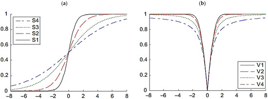
Figure 2.
(a) S-shaped TFs; (b) V-shaped TFs.
3.3. Knapsack Problems
The 0-1 Knapsack Problem (KP) is a classical combinatorial optimization problem that involves selecting a subset of items from a larger set to maximize overall profit within a specific weight limit [32]. Each item is associated with a specific weight and profit, and a binary variable determines whether it is included in the knapsack. The objective is to maximize total profit while ensuring that the total weight of the selected items does not exceed the knapsack capacity [49]. In this representation, a value of “1” indicates that an item is selected, whereas a value of “0” indicates that it is not. This binary encoding efficiently represents potential solutions, enabling the optimization process to balance capacity utilization and profit maximization [16]. Finally, 0-1 KPs can mathematically be formulated as:
where is the total number of items, is the weight of the item, is the profit, is the maximum capacity of the knapsack. This subset of items can be identified by constructing a knapsack that contains the selected item with a value of = 1, while the other items have a value of = 0 and are not selected for the knapsack [33].
3.4. Penalty Algorithm
Infeasible solutions occur when their total weight exceeds the capacity constraint. In such cases, a Penalty Algorithm (PA) is applied to prevent the solution from being selected, even though it provides a high profit. In this approach, the fitness value of each infeasible solution is converted to a negative value so that the algorithm does not prefer this solution as the best candidate [33]. Figure 3 depicts the pseudo-code of the PA.
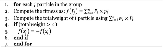
Figure 3.
Pseudo-code of PA [33].
3.5. Fixing Infeasible Solution
The Repair Algorithm (RA) and the Improvement Algorithm (IA) constitute two essential procedures for refining candidate solutions in binary optimization. The RA is primarily responsible for restoring feasibility by correcting solutions that violate problem-specific constraints, such as exceeding the knapsack capacity. It systematically adjusts the solution structure to ensure compliance with the feasibility requirements of the problem. Once feasibility is achieved, the IA operates to enhance the overall solution quality. This is accomplished by strategically modifying feasible solutions such as replacing or reordering selected items in order to increase total profit while maintaining constraint satisfaction. Collectively, these two procedures form a complementary mechanism: the RA ensures the validity of solutions, while the IA improves their effectiveness within the feasible search space [33].
In RA, items are prioritized for removal based on their profit-to-weight ratio (), with the item having the lowest ratio eliminated first. In the case of ties, the item with the smallest absolute profit is removed. This process is repeated until the total weight satisfies the knapsack capacity. The pseudo-code of RA is presented in Figure 4.
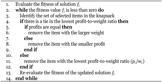
Figure 4.
Pseudo-code of RA [33].
In the IA, when multiple items have equal ratios, the item with the highest profit is selected. After each addition, the objective function is recalculated. To reduce computational cost, IA evaluates only the top-ranked subset of the remaining items. If the updated solution becomes infeasible, the last added item is removed and the process is terminated. The pseudo-code of IA is provided in Figure 5 [33].
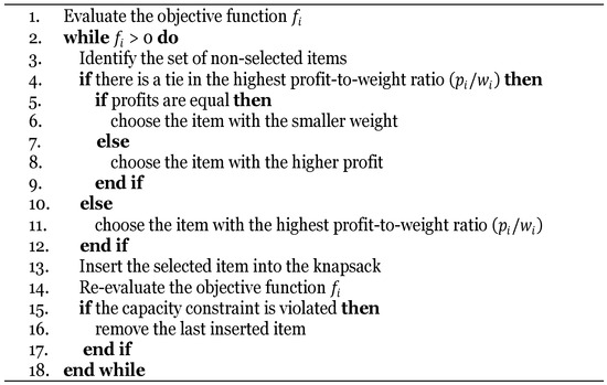
Figure 5.
Pseudo-code of IA [33].
3.6. Uncapacitated Facility Location Problem
Assuming that there is no capacity limit on facilities and that each customer is served by only one facility, the Uncapacitated Facility Location Problem (UFLP) entails offering consumers a selection of facilities. The location of factories, warehouses, or power transmission lines is a critical location decision problem [50,51]. The UFLP entails evaluating the location of facilities and the associated expenses of customer service. The primary objective is to minimize the overall cost of business operations by meticulously organizing the layout of facilities [42]. UFLP solutions are found by using a binary vector to indicate whether each facility is open or closed and examining various ways to arrange the facilities. The larger the dimensions of a problem, the harder it becomes. The UFLP is an NP-hard problem [52]. The primary objective is to ascertain the most appropriate locations for the facilities and the most effective methods of serving the clients, thereby reducing the company’s overall operating expenses [53]. The objective function is the total cost of providing services to customers and opening the facilities. The objective is to determine the most cost-effective method of assigning facilities to customers [54]. A mathematical definition of the UFLP is provided in Equation (40).
where indicates whether -th customer receives service from -th facility. indicates whether -th facility is open. is the number of consumers, and is the number of facilities. The serviceCostij represents the service cost that -th consumer receives from the -th facility, represents the opening cost required by the opening of the -th facility [42].
3.7. Crossover Operation
Crossover is a genetic operator widely used in evolutionary and metaheuristic algorithms. It produces new offspring solutions by combining genetic information from two parent solutions according to predefined rules. This process aims to increase diversity in the search space, facilitate information exchange from high-quality solutions, and improve the overall performance of the algorithm [55,56]. Crossover operators can be implemented through different strategies:
- One-point crossover: A random cut-point is selected, and all genes beyond this point are exchanged between the two parent solutions.
- Two-point crossover: Two crossover points are selected randomly, and the segment between them is swapped between the parent solutions.
- Uniform crossover: Each gene is independently inherited from one of the parent solutions with a predefined probability.
In general, crossover enhances information sharing among solutions, preserves diversity, and strengthens the exploitation capability of the algorithm [57]. In this study, a hybrid crossover approach governed by the crossover probability (pCR) is adopted. In this mechanism, a random crossover point is selected to ensure that at least one gene from the candidate solution is transferred to the offspring, thereby guaranteeing structural diversity and preventing the production of identical offspring. For the remaining genes, the uniform crossover principle is applied, where each gene is independently inherited from either the candidate or the current solution, according to the probability pCR. For example, when pCR = 0.2, approximately 20% of the genes are expected to be inherited from the candidate solution and 80% from the parent solution. Moreover, to prevent invalid offspring (e.g., all-zero vectors), at least one element is enforced to remain active. This additional mechanism guarantees feasibility and eliminates the generation of meaningless solutions.
3.8. Greedy-Based Population Strategies
The greedy-based population strategy is widely employed to generate high-quality initial solutions in combinatorial optimization problems such as the 0-1 KPs. In this strategy, items are ranked according to their profit-to-weight ratio, and those with higher efficiency are selected first to construct candidate solutions. This ensures that the initial population is composed of solutions with relatively good objective values, which can accelerate convergence in the subsequent search process. To prevent premature convergence and preserve diversity, random perturbations (noise) are incorporated into the greedy ordering. By combining deterministic efficiency-based selection with controlled randomness, this approach strikes a balance between solution quality and population diversity, thereby enhancing the overall effectiveness of the optimization process [58,59].
The greedy-based population strategy is designed to generate high-quality yet diverse solutions in the initial population. For each item, the profit-to-weight ratio () is first calculated to measure its efficiency. To avoid deterministic ordering that could lead to a homogeneous population, a small random noise is added to these efficiency values. The items are then sorted in descending order based on the perturbed efficiency scores. Following this ranking, items are sequentially inserted into the knapsack as long as the total weight does not exceed the capacity. In this way, the most efficient items are selected first, and the process continues until the knapsack is filled. This strategy ensures that the generated solutions are feasible with respect to the capacity constraint while maintaining the high-profit tendency of the greedy principle. Furthermore, the introduction of random noise preserves diversity within the population, prevents premature convergence, and contributes to a more balanced algorithm between exploration and exploitation throughout the optimization process [59].
In conclusion, the greedy-based population strategy ensures the generation of high-quality solutions, while the incorporation of random noise preserves diversity within the population. This combination provides a robust starting point that supports both exploration and exploitation capabilities in subsequent iterations of the algorithm.
4. The Binary Puma Optimizer
In this study, two distinct variants of the proposed Binary Puma Optimizer (BPO) have been developed. These variants have been designed using TFs (four S-shaped and four V-shaped) and are tailored for the 0-1 Knapsack Problem (KP) and Uncapacitated Facility Location Problem (UFLP). The following subsections describe the structural characteristics and design details of the proposed BPO and BPO’s variants.
4.1. TFs-Based Binary Transformation
In the standard BPO framework, the continuous candidate solution is subsequently mapped into the binary domain. Specifically, the selected TFs transform each continuous value into a probability within the interval . Then, this probability is compared with a uniformly distributed random number rand to decide the binary state of each dimension. In this study, eight TFs comprising four S-shaped and four V-shaped functions are investigated to assess their effectiveness in guiding the search process within the binary domain. Accordingly, BPO1 converts continuous values into binary representations to solve the 0-1 KPs. The binarization process is expressed in Equation (41).
where denotes the value of the dim-th component of the -th candidate solution. represents the TFs that maps a continuous value into a probability in the range , while rand is a uniformly distributed random variable within .
4.2. Binary Puma Optimizer-1 for 0-1 KP
A novel algorithm, termed the Binary Puma Optimizer-1 (BPO1), is proposed in this study as a binary adaptation of the BPO, which is initially designed for continuous domains. Since the direct application of BPO to binary optimization problems, such as the 0-1 KP, is not feasible, both the initialization strategies and the iterative update mechanisms of the algorithm have been redesigned and augmented with TFs specifically tailored for the binary search space.
Given the characteristics of the 0-1 KP, infeasible solutions frequently violate the capacity constraint. When such violations are addressed solely through penalty functions, solution quality tends to deteriorate, leading to inefficiencies in the search process. To overcome this limitation, BPO1 employs different mechanisms. These mechanisms not only ensure feasibility but also improve the overall quality of solutions, thereby enhancing the algorithm’s effectiveness in solving constrained binary optimization problems.
4.2.1. Greedy-Based Populations Strategies and TFs-Based Binary Transformation
The quality of the initial population strongly influences the efficiency of the search process. To address this, BPO1 employs a hybrid initialization strategy that ensures both diversity and solution quality.
- Random populations: Half of the population is generated as random solutions that strictly satisfy the capacity constraint. This approach enhances diversity by introducing a wide range of candidate solutions.
- Greedy-based populations strategies: The remaining half is constructed using a greedy strategy in which items are ranked according to their profit-to-weight ratio. This ensures that solutions are biased toward higher quality in terms of profitability.
By combining random and greedy-based strategies, the hybrid population initialization provides high-quality candidate solutions in the early stages while maintaining sufficient exploratory capacity to guide the search toward the global optimum. Furthermore, once the candidate solutions are generated, they are transformed into the binary domain using the TFs-based binarization procedure expressed in Equation (41). This process ensures that continuous values are effectively converted into binary representations, thereby enabling BPO1 to operate efficiently within the 0-1 search space.
4.2.2. Crossover Operator
The newly generated candidate solution, y is recombined with the current solution, x, through a crossover operator. This procedure is executed as follows:
- A random position j0 is selected, and the corresponding component is always inherited from y, ensuring that the offspring differs from the parent.
- For all other dimensions, values are inherited from y with a predefined crossover probability pCR otherwise, the values of x are retained.
- As a result, the offspring solution z combines the features of both the parent solution x and the candidate solution y.
- To prevent the generation of empty solutions (i.e., solutions with no selected items), at least one item is enforced by randomly assigning a value of 1 to one position if necessary.
This crossover operator maintains population diversity while simultaneously enabling information exchange between parent and candidate solutions, thereby contributing to the effective guidance of the evolutionary search process.
4.2.3. Penalty, Repair, and Improvement Algorithm
Due to the inherent nature of the 0-1 KPs, violations of the capacity constraint frequently result in infeasible solutions. To address this problem, BPO1 employs a three-stage constraint-handling mechanism composed of the following procedures:
- Penalty Algorithm (PA): Infeasible solutions that exceed the capacity constraint are penalized according to the degree of violation. This reduces their fitness values and decreases their likelihood of being selected in subsequent iterations.
- Repair Algorithm (RA): Infeasible solutions are iteratively corrected by removing items with the lowest profit-to-weight ratio until the total weight satisfies the knapsack capacity, thereby restoring feasibility.
- Improvement Algorithm (IA): Once feasibility is ensured, solutions are further refined by incorporating items with the highest profit-to-weight ratio, provided the capacity constraint is not violated. This process increases the overall profit and enhances solution quality.
BPO1 is proposed as a binary adaptation of the original PO, redesigned to address the specific requirements of 0-1 KPs. To generate a strong starting point, BPO1 employs a hybrid initialization strategy that combines random feasible solutions with greedy-based solutions guided by profit-to-weight ratios, ensuring both diversity and quality. Continuous candidate solutions are transformed into binary form using eight TFs, including four S-shaped and four V-shaped mappings. A tailored crossover operator enables effective information exchange between parent and candidate solutions while preserving diversity. To handle infeasible solutions, BPO1 integrates a three-stage mechanism: infeasible solutions are first penalized, then repaired by eliminating low-efficiency items, and finally improved through greedy insertion of high-efficiency items. Collectively, these mechanisms ensure feasibility, enhance solution quality, and improve the algorithm’s overall effectiveness in solving complex constrained binary optimization problems. The flowchart of the proposed BPO1 algorithm applied to 0-1 KPs is presented in Figure 6. Figure 7 presents the step-by-step pseudo-code of the proposed BPO1 algorithm designed for solving 0-1 KPs.
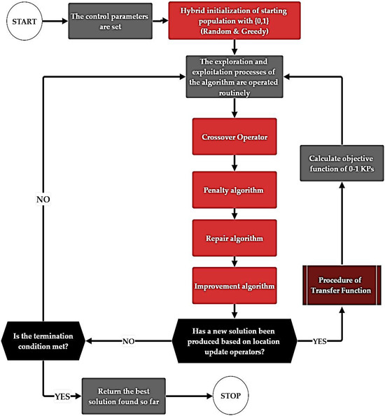
Figure 6.
Flowchart of BPO1 for 0-1 KPs.
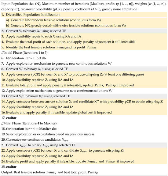
Figure 7.
Pseuduo-code of BPO1 for 0-1 KPs.
4.3. Binary Puma Optimizer-2 for UFLP
Secondly, this study introduces the Binary Puma Optimizer-2 (BPO2), a binary adaptation of the BPO specifically designed to solve the UFLP. Similarly to other binary variants of metaheuristic algorithms, BPO2 utilizes TFs as the primary mechanism for mapping continuous update values into binary decision variables. In this study, eight TFs are examined, including four S-shaped and four V-shaped mappings.
For the UFLP, the adaptation procedure follows the same principle applied in other binary algorithms. The initial population is generated directly as binary vectors to represent facility-opening and assignment decisions, thereby eliminating unnecessary transformation steps. During subsequent iterations, candidate solutions are updated using the exploration and exploitation operators of the original PO. The resulting continuous values are then passed through the selected TFs, which transform them into probabilities within the interval . Each probability is compared against a uniformly distributed random number rand , and the binary state of each dimension is then determined using the binarization rule in Equation (41).
Once binary solutions are generated, they are evaluated using the UFLP objective function, which minimizes total facility-opening and assignment costs. The best-performing solutions are retained through selection mechanisms, guiding the population toward more cost-efficient configurations.
The cycle of continuous updating, TFs based binarization, and solution evaluation is repeated across generations until the termination criterion is satisfied, either by reaching a predefined number of iterations or by achieving convergence.
In the UFLP, facility-opening (0-1) and assignment decisions are not subject to capacity restrictions, since each facility is assumed to have unlimited capacity. As a result, no infeasible solutions arise from exceeding resource limits, and corrective mechanisms such as the PA, RA, and IA are not required. In contrast, in the 0–1 KP, each item selection directly affects the total weight, and exceeding the knapsack capacity produces infeasible solutions. Under such circumstances, PAs are needed to discourage constraint violations, RAs are required to restore feasibility by removing low-efficiency items, and IAs are applied to further enhance feasible solutions by inserting high-efficiency items. Collectively, these algorithms are indispensable in KPs to ensure feasibility and maintain solution quality, whereas in the UFLP, they become redundant due to the absence of capacity constraints. Figure 8 illustrates the flowchart of the proposed BPO applied to the UFLP, while Figure 9 presents the step-by-step pseudo-code of the proposed BPO2 for solving the UFLP. The gray colors in Figure 9 represent the binary adaptation of BPO2.
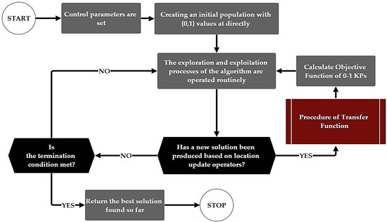
Figure 8.
Flowchart of the BPO2 for the UFLP.
Figure 9.
Pseudo-code of BPO2 for UFLP.
5. Results
Transfer Functions (TFs) are categorized based on their problem size and difficulty level, ranging from small to huge. This categorization ensures a diverse and comprehensive evaluation of the optimization algorithm’s performance across varying problem complexities. The GAP value is formulated mathematically by Equation (42) [42]. The Success Rate (SR) is calculated by Equation (43) [33]:
5.1. Experimental Results of BPO1 for 0-1 KPs
Table 3 shows the BPO1 parameter values used in the experiments. The OR Library [33] provides a comprehensive 0-1 KPs dataset comprising 25 distinct datasets detailed in Table 4. In the table, “ID” refers to the instance number assigned in this study, while Dataset denotes the name of the benchmark instance (e.g., 8a, 12b, 20c). Cap. Indicates the knapsack capacity associated with each dataset, and “Dim.” represents the problem dimension. Finally, “Opt.” corresponds to the known optimal objective value of each dataset. Table 5, Table 6, Table 7, Table 8, Table 9, Table 10, Table 11 and Table 12 present the statistical results of BPO1. In the tables, “Dataset” denotes the problem dataset, “Cap.” refers to the knapsack capacity, and “Opt.” represents the known optimal value. “Best” indicates the maximum profit achieved, “Mean” is the average profit across multiple runs, and Worst denotes the minimum profit obtained. “Std.” Corresponds to the standard deviation of the results. “Weight” refers to the total weight of the items included in the best solution, and “WR” (weight ratio) expresses the percentage of the knapsack capacity utilized. “Time” is reported as the average computational time per run. Finally, “SR” represents the success rate, defined as the percentage of independent runs in which at least one feasible solution satisfying all problem constraints is generated. In the tables, the use of bold font is intended to denote the optimum value.
Table 3.
Parameter settings.
Table 3.
Parameter settings.
| Parameters | Values |
|---|---|
| Population size (N) | 20 |
| Maximum iteration (MaxIter) | 5000 |
| Number of runs | 20 |
| Crossover probability (pCR) | 0.20 |
| Greedy noise amplitude parameter | 0.10 |
Table 4.
Datasets of instances for the 0-1 KPs [31].
Table 4.
Datasets of instances for the 0-1 KPs [31].
| ID | Dataset | Cap. | Dim. | Opt. |
|---|---|---|---|---|
| KP(1) | 8a | 1,863,633 | 8 | 3,924,400 |
| KP(2) | 8b | 1,822,718 | 8 | 3,813,669 |
| KP(3) | 8c | 1,609,419 | 8 | 3,347,452 |
| KP(4) | 8d | 2,112,292 | 8 | 4,187,707 |
| KP(5) | 8e | 2,493,250 | 8 | 4,955,555 |
| KP(6) | 12a | 2,805,213 | 12 | 5,688,887 |
| KP(7) | 12b | 3,259,036 | 12 | 6,498,597 |
| KP(8) | 12c | 3,489,815 | 12 | 5,170,626 |
| KP(9) | 12d | 3,453,702 | 12 | 6,992,404 |
| KP(10) | 12e | 2,520,392 | 12 | 5,337,472 |
| KP(11) | 16a | 3,780,355 | 16 | 7,850,983 |
| KP(12) | 16b | 4,426,945 | 16 | 9,352,998 |
| KP(13) | 16c | 4,323,280 | 16 | 9,151,147 |
| KP(14) | 16d | 4,550,938 | 16 | 9,348,889 |
| KP(15) | 16e | 3,760,429 | 16 | 7,769,117 |
| KP(16) | 20a | 5,169,647 | 20 | 10,727,049 |
| KP(17) | 20b | 4,681,373 | 20 | 9,818,261 |
| KP(18) | 20c | 5,063,791 | 20 | 10,714,023 |
| KP(19) | 20d | 4,286,641 | 20 | 8,929,156 |
| KP(20) | 20e | 4,476,000 | 20 | 9,357,969 |
| KP(21) | 24a | 6,404,180 | 24 | 13,549,094 |
| KP(22) | 24b | 5,971,071 | 24 | 12,233,713 |
| KP(23) | 24c | 5,870,470 | 24 | 12,448,780 |
| KP(24) | 24d | 5,762,284 | 24 | 11,815,315 |
| KP(25) | 24e | 6,654,569 | 24 | 13,940,099 |
Table 5.
The results of the BPO1 for TF1.
Table 5.
The results of the BPO1 for TF1.
| Dataset | Cap. | Opt. | Best | Mean | Worst | Std. | Weight | WR | Time | SR |
|---|---|---|---|---|---|---|---|---|---|---|
| 8a | 1,863,633 | 3,924,400 | 3,924,400 | 3,924,400 | 3,924,400 | 0 | 1,826,529 | 98.0091 | 1.8722 | 100 |
| 8b | 1,822,718 | 3,813,669 | 3,813,669 | 3,813,669 | 3,813,669 | 0 | 1,809,614 | 99.2811 | 1.8669 | 100 |
| 8c | 1,609,419 | 3,347,452 | 3,347,452 | 3,347,452 | 3,347,452 | 0 | 1,598,893 | 99.3460 | 1.8644 | 100 |
| 8d | 2,112,292 | 4,187,707 | 4,187,707 | 4,187,707 | 4,187,707 | 0 | 2,048,957 | 97.0016 | 1.8647 | 100 |
| 8e | 2,493,250 | 4,955,555 | 4,955,555 | 4,955,555 | 4,955,555 | 0 | 2,442,114 | 97.9490 | 1.8629 | 100 |
| 12a | 2,805,213 | 5,688,887 | 5,688,887 | 5,688,887 | 5,688,887 | 0 | 2,798,038 | 99.7442 | 1.9166 | 100 |
| 12b | 3,259,036 | 6,498,597 | 6,498,597 | 6,497,318 | 6,473,019 | 5719 | 3,256,963 | 99.9364 | 1.9003 | 100 |
| 12c | 2,489,815 | 5,170,626 | 5,170,626 | 5,170,626 | 5,170,626 | 0 | 2,470,810 | 99.2367 | 1.8899 | 100 |
| 12d | 3,453,702 | 6,992,404 | 6,992,404 | 6,992,404 | 6,992,404 | 0 | 3,433,409 | 99.4124 | 1.8822 | 100 |
| 12e | 2,520,392 | 5,337,472 | 5,337,472 | 5,337,472 | 5,337,472 | 0 | 2,514,881 | 99.7813 | 1.879 | 100 |
| 16a | 3,780,355 | 7,850,983 | 7,850,983 | 7,842,093 | 7,823,318 | 11,500 | 3,771,406 | 99.7633 | 1.9549 | 100 |
| 16b | 4,426,945 | 9,352,998 | 9,352,998 | 9,347,804 | 9,259,634 | 20,816 | 4,426,267 | 99.9847 | 1.9440 | 100 |
| 16c | 4,323,280 | 9,151,147 | 9,151,147 | 9,147,364 | 9,100,116 | 12,406 | 4,297,175 | 99.3962 | 1.9526 | 100 |
| 16d | 4,450,938 | 9,348,889 | 9,348,889 | 9,338,199 | 9,305,859 | 9316 | 4,444,721 | 99.8603 | 1.9536 | 100 |
| 16e | 3,760,429 | 7,769,117 | 7,769,117 | 7,764,839 | 7,750,491 | 7661 | 3,752,854 | 99.7986 | 1.9544 | 100 |
| 20a | 5,169,647 | 10,727,049 | 10,727,049 | 10,725,302 | 10,692,101 | 7815 | 5,166,676 | 99.9425 | 2.0298 | 100 |
| 20b | 4,681,373 | 9,818,261 | 9,818,261 | 9,809,366 | 9,754,368 | 16,503 | 4,671,869 | 99.7970 | 2.0368 | 100 |
| 20c | 5,063,791 | 10,714,023 | 10,714,023 | 10,710,007 | 10,700,635 | 6295 | 5,053,832 | 99.8033 | 2.0303 | 100 |
| 20d | 4,286,641 | 8,929,156 | 8,929,156 | 8,921,022 | 8,873,716 | 17,171 | 4,282,619 | 99.9062 | 2.0276 | 100 |
| 20e | 4,476,000 | 9,357,969 | 9,357,969 | 9,355,219 | 9,345,847 | 4762 | 4,470,060 | 99.8673 | 2.0312 | 100 |
| 24a | 6,404,180 | 13,549,094 | 13,549,094 | 13,511,191 | 13,459,475 | 26,876 | 6,402,560 | 99.9747 | 2.0987 | 100 |
| 24b | 5,971,071 | 12,233,713 | 12,233,713 | 12,215,824 | 12,159,261 | 24,149 | 5,966,008 | 99.9152 | 2.1076 | 100 |
| 24c | 5,870,470 | 12,448,780 | 12,448,780 | 12,435,421 | 12,367,653 | 20,381 | 5,861,707 | 99.8507 | 2.0966 | 100 |
| 24d | 5,762,284 | 11,815,315 | 11,815,315 | 1,180,541 | 11,754,633 | 19,258 | 5,756,602 | 99.9014 | 2.1036 | 100 |
| 24e | 6,654,569 | 13,940,099 | 13,940,099 | 13,933,446 | 13,909,292 | 9135 | 6,637,749 | 99.7472 | 2.0966 | 100 |
The bolded values indicate the optimum value.
In Table 5, the performance of BPO1 with TF1 across the 0-1 KPs is reported. Across all datasets, the Best values are found to be identical to the known optima, indicating that BPO1 successfully identified the optimal solution in every run. For the datasets ranging from 8a to 12e, the mean values are consistently matched with the optimal results, except for instance 12b, where a slight deviation is observed. Within the same range (8a–12e), the standard deviation is recorded as zero, confirming the complete stability of the algorithm except for instance 12b. For larger-scale instances, small variations in the mean values and standard deviation are observed; however, these deviations are considered negligible and do not compromise the algorithm’s overall robustness. Capacity utilization rates exceeded 97%, with most rates above 99%, demonstrating efficient resource use. The success rate is 100% for all datasets. These findings confirm that the proposed algorithm delivers high accuracy, stability, and efficiency across problems of varying scales, including large-scale instances.
Table 6.
The results of the BPO1 for TF2.
Table 6.
The results of the BPO1 for TF2.
| Dataset | Cap. | Opt. | Best | Mean | Worst | Std. | Weight | WR | Time | SR |
|---|---|---|---|---|---|---|---|---|---|---|
| 8a | 1,863,633 | 3,924,400 | 3,924,400 | 3,924,400 | 3,924,400 | 0 | 1,826,529 | 98.0090 | 1.8589 | 100 |
| 8b | 1,822,718 | 3,813,669 | 3,813,669 | 3,813,669 | 3,813,669 | 0 | 1,809,614 | 99.2810 | 1.8556 | 100 |
| 8c | 1,609,419 | 3,347,452 | 3,347,452 | 3,347,452 | 3,347,452 | 0 | 1,598,893 | 99.3459 | 1.8708 | 100 |
| 8d | 2,112,292 | 4,187,707 | 4,187,707 | 4,187,707 | 4,187,707 | 0 | 2,048,957 | 97.0016 | 1.8779 | 100 |
| 8e | 2,493,250 | 4,955,555 | 4,955,555 | 4,955,555 | 4,955,555 | 0 | 2,442,114 | 97.9490 | 1.8776 | 100 |
| 12a | 2,805,213 | 5,688,887 | 5,688,887 | 5,688,887 | 5,688,887 | 0 | 2,798,038 | 99.7442 | 1.9298 | 100 |
| 12b | 3,259,036 | 6,498,597 | 6,498,597 | 6,498,597 | 6,498,597 | 0 | 3,256,963 | 99.9364 | 1.9295 | 100 |
| 12c | 2,489,815 | 5,170,626 | 5,170,626 | 5,170,626 | 5,170,626 | 0 | 2,470,810 | 99.2367 | 1.9353 | 100 |
| 12d | 3,453,702 | 6,992,404 | 6,992,404 | 6,992,404 | 6,992,404 | 0 | 3,433,409 | 99.4124 | 1.9472 | 100 |
| 12e | 2,520,392 | 5,337,472 | 5,337,472 | 5,337,472 | 5,337,472 | 0 | 2,514,881 | 99.7813 | 1.9338 | 100 |
| 16a | 3,780,355 | 7,850,983 | 7,850,983 | 7,840,710 | 7,823,318 | 12,026 | 3,771,406 | 99.7634 | 1.9753 | 100 |
| 16b | 4,426,945 | 9,352,998 | 9,352,998 | 9,352,208 | 9,347,736 | 1927 | 4,426,267 | 99.9846 | 1.9689 | 100 |
| 16c | 4,323,280 | 9,151,147 | 9,151,147 | 9,146,133 | 9,100,116 | 13,206 | 4,297,175 | 99.3962 | 1.9691 | 100 |
| 16d | 4,450,938 | 9,348,889 | 9,348,889 | 9,333,429 | 9,296,536 | 14,043 | 4,444,721 | 99.8603 | 1.9784 | 100 |
| 16e | 3,760,429 | 7,769,117 | 7,769,117 | 7,761,303 | 7,750,491 | 8948 | 3,752,854 | 99.7986 | 1.9716 | 100 |
| 20a | 5,169,647 | 10,727,049 | 10,727,049 | 10,725,302 | 10,692,101 | 7815 | 5,166,676 | 99.9425 | 2.0300 | 100 |
| 20b | 4,681,373 | 9,818,261 | 9,818,261 | 9,809,732 | 9,753,772 | 17,625 | 4,671,869 | 99.7969 | 2.0332 | 100 |
| 20c | 5,063,791 | 10,714,023 | 10,714,023 | 10,706,515 | 10,700,635 | 6682 | 5,053,832 | 99.8033 | 2.0237 | 100 |
| 20d | 4,286,641 | 8,929,156 | 8,929,156 | 8,919,512 | 8,873,716 | 17,677 | 4,282,619 | 99.9062 | 2.0184 | 100 |
| 20e | 4,476,000 | 9,357,969 | 9,357,969 | 9,354,550 | 9,345,847 | 5165 | 4,470,060 | 99.8673 | 2.0234 | 100 |
| 24a | 6,404,180 | 13,549,094 | 13,549,094 | 13,515,169 | 13,460,329 | 26,859 | 6,402,560 | 99.9747 | 2.0913 | 100 |
| 24b | 5,971,071 | 12,233,713 | 12,233,713 | 12,220,570 | 12,159,261 | 21,267 | 5,966,008 | 99.9152 | 2.0926 | 100 |
| 24c | 5,870,470 | 12,448,780 | 12,448,780 | 12,429,256 | 12,385,452 | 20,738 | 5,861,707 | 99.8507 | 2.0866 | 100 |
| 24d | 5,762,284 | 11,815,315 | 11,815,315 | 11,806,293 | 11,772,086 | 13,984 | 5,756,602 | 99.9014 | 2.0940 | 100 |
| 24e | 6,654,569 | 13,940,099 | 13,940,099 | 13,933,005 | 13,902,534 | 12,358 | 6,637,749 | 99.7472 | 2.0888 | 100 |
Table 6 presents the performance of the proposed algorithm using TF2 across all 0-1 KPs. For the 8a–12e datasets, the algorithm consistently achieved the optimal solution in all runs, with best, mean, and worst values identical and a standard deviation of zero, indicating perfect stability. In the larger datasets (16a–24e), the best results always matched the optimum, and the mean and worst results remained extremely close to it, with very small standard deviations, demonstrating strong robustness. Capacity utilization ratios ranged from approximately 97% to nearly 100%, confirming efficient use of available resources. Execution times remained low across all datasets, and the success rate is 100% in every case. These results indicate that, under TF2, the proposed algorithm maintains high accuracy, stability, and efficiency across different problem sizes, including large-scale instances. This advantage is attributed to TF2′s probability curve being more balanced in the middle region, thereby enabling a more effective balance between exploration and exploitation phases. The probability curves of TF1 and TF2 exhibit a more balanced distribution in the middle region. This characteristic enables a more effective balance between the exploration and exploitation phases, yielding stable results in small- and medium-scale datasets and slightly more consistent performance in large-scale datasets.
Table 7.
The results of the BPO1 for TF3.
Table 7.
The results of the BPO1 for TF3.
| Dataset | Cap. | Opt. | Best | Mean | Worst | Std. | Weight | WR | Time | SR |
|---|---|---|---|---|---|---|---|---|---|---|
| 8a | 1,863,633 | 3,924,400 | 3,924,400 | 3,924,400 | 3,924,400 | 0 | 1,826,529 | 98.0090 | 1.8669 | 100 |
| 8b | 1,822,718 | 3,813,669 | 3,813,669 | 3,813,669 | 3,813,669 | 0 | 1,809,614 | 99.2810 | 1.8685 | 100 |
| 8c | 1,609,419 | 3,347,452 | 3,347,452 | 3,347,452 | 3,347,452 | 0 | 1,598,893 | 99.3459 | 1.8606 | 100 |
| 8d | 2,112,292 | 4,187,707 | 4,187,707 | 4,187,707 | 4,187,707 | 0 | 2,048,957 | 97.0015 | 1.8631 | 100 |
| 8e | 2,493,250 | 4,955,555 | 4,955,555 | 4,955,555 | 4,955,555 | 0 | 2,442,114 | 97.9490 | 1.8658 | 100 |
| 12a | 2,805,213 | 5,688,887 | 5,688,887 | 5,688,887 | 5,688,887 | 0 | 2,798,038 | 99.7442 | 1.9573 | 100 |
| 12b | 3,259,036 | 6,498,597 | 6,498,597 | 6,494,760 | 6,473,019 | 9370 | 3,256,963 | 99.9363 | 1.9496 | 100 |
| 12c | 2,489,815 | 5,170,626 | 5,170,626 | 5,170,626 | 5,170,626 | 0 | 2,470,810 | 99.2366 | 1.9552 | 100 |
| 12d | 3,453,702 | 6,992,404 | 6,992,404 | 6,992,404 | 6,992,404 | 0 | 3,433,409 | 99.4124 | 1.9491 | 100 |
| 12e | 2,520,392 | 5,337,472 | 5,337,472 | 5,337,472 | 5,337,472 | 0 | 2,514,881 | 99.7813 | 1.9449 | 100 |
| 16a | 3,780,355 | 7,850,983 | 7,850,983 | 7,845,372 | 7,823,318 | 10,207 | 3,771,406 | 99.7632 | 2.0082 | 100 |
| 16b | 4,426,945 | 9,352,998 | 9,352,998 | 9,352,998 | 9,352,998 | 0 | 4,426,267 | 99.9847 | 2.0053 | 100 |
| 16c | 4,323,280 | 9,151,147 | 9,151,147 | 9,143,922 | 9,082,307 | 19,064 | 4,297,175 | 99.3965 | 2.0108 | 100 |
| 16d | 4,450,938 | 9,348,889 | 9,348,889 | 9,338,342 | 9,296,536 | 11,357 | 4,444,721 | 99.8603 | 2.0046 | 100 |
| 16e | 3,760,429 | 7,769,117 | 7,769,117 | 7,765,217 | 7,750,491 | 6973 | 3,752,854 | 99.7985 | 2.0055 | 100 |
| 20a | 5,169,647 | 10,727,049 | 10,727,049 | 10,723,554 | 10,692,101 | 10,756 | 5,166,676 | 99.9425 | 2.0566 | 100 |
| 20b | 4,681,373 | 9,818,261 | 9,818,261 | 9,805,114 | 9,744,513 | 23,273 | 4,671,869 | 99.7969 | 2.0480 | 100 |
| 20c | 5,063,791 | 10,714,023 | 10,714,023 | 10,702,726 | 10,611,486 | 22,453 | 5,053,832 | 99.8033 | 2.0245 | 100 |
| 20d | 4,286,641 | 8,929,156 | 8,929,156 | 89,267,678 | 8,895,152 | 8050 | 4,282,619 | 99.9061 | 2.0224 | 100 |
| 20e | 4,476,000 | 9,357,969 | 9,357,969 | 93,564,304 | 9,345,847 | 3560 | 4,470,060 | 99.8673 | 2.0238 | 100 |
| 24a | 6,404,180 | 13,549,094 | 13,549,094 | 13,516,478 | 13,455,545 | 28,966 | 6,402,560 | 99.9747 | 2.0851 | 100 |
| 24b | 5,971,071 | 12,233,713 | 12,233,713 | 12,221,969 | 12,193,732 | 15,937 | 5,966,008 | 99.9152 | 2.0853 | 100 |
| 24c | 5,870,470 | 12,448,780 | 12,448,780 | 12,439,973 | 12,401,619 | 13,640 | 5,861,707 | 99.8507 | 2.0861 | 100 |
| 24d | 5,762,284 | 11,815,315 | 11,815,315 | 11,801,226 | 11,754,633 | 19,256 | 5,756,602 | 99.9013 | 2.0881 | 100 |
| 24e | 6,654,569 | 13,940,099 | 13,940,099 | 13,925,645 | 13,902,534 | 12,720 | 6,637,749 | 99.7472 | 2.0800 | 100 |
As shown in Table 7, TF3 is reported to have achieved high accuracy across most datasets, although slight deviations in mean and worst values are observed in datasets 12b and 16a. These deviations are considered to be due to TF3′s structure being less capable than TF2 of sustaining strong local search intensity for certain problem sizes. While TF3 is observed to be more stable compared to TF1, it does not achieve the same low variance levels as TF2 and TF4. Nevertheless, the high-capacity utilization ratios indicate that the overall solution quality is maintained.
TF2 and TF3 exhibit high-capacity utilization rates (97–100%) while maintaining overall solution quality. However, TF2 demonstrates a more stable and consistent performance than TF3 by delivering near-zero variance and perfect stability across both small-to-medium and large-scale problems. Although TF3 achieves high accuracy in most datasets, minor deviations in mean and worst-case values are observed in datasets 12b and 16a. These deviations can be attributed to TF3′s inability to sustain local search intensity as effectively as TF2 for certain problem sizes.
Table 8.
The results of the BPO1 for TF4.
Table 8.
The results of the BPO1 for TF4.
| Dataset | Cap. | Opt. | Best | Mean | Worst | Std. | Weight | WR | Time | SR |
|---|---|---|---|---|---|---|---|---|---|---|
| 8a | 1,863,633 | 3,924,400 | 3,924,400 | 3,924,400 | 3,924,400 | 0 | 1,826,529 | 98.0091 | 1.8785 | 100 |
| 8b | 1,822,718 | 3,813,669 | 3,813,669 | 3,813,669 | 3,813,669 | 0 | 1,809,614 | 99.2810 | 1.8785 | 100 |
| 8c | 1,609,419 | 3,347,452 | 3,347,452 | 3,347,452 | 3,347,452 | 0 | 1,598,893 | 99.3459 | 1.8731 | 100 |
| 8d | 2,112,292 | 4,187,707 | 4,187,707 | 4,187,707 | 4,187,707 | 0 | 2,048,957 | 97.0015 | 1.8768 | 100 |
| 8e | 2,493,250 | 4,955,555 | 4,955,555 | 4,955,555 | 4,955,555 | 0 | 2,442,114 | 97.9490 | 1.8751 | 100 |
| 12a | 2,805,213 | 5,688,887 | 5,688,887 | 5,688,887 | 5,688,887 | 0 | 2,798,038 | 99.7442 | 1.9466 | 100 |
| 12b | 3,259,036 | 6,498,597 | 6,498,597 | 6,498,597 | 6,498,597 | 0 | 3,256,963 | 99.9363 | 1.9293 | 100 |
| 12c | 2,489,815 | 5,170,626 | 5,170,626 | 5,170,626 | 5,170,626 | 0 | 2,470,810 | 99.2366 | 1.9393 | 100 |
| 12d | 3,453,702 | 6,992,404 | 6,992,404 | 6,992,404 | 6,992,404 | 0 | 3,433,409 | 99.4124 | 1.9327 | 100 |
| 12e | 2,520,392 | 5,337,472 | 5,337,472 | 5,337,472 | 5,337,472 | 0 | 2,514,881 | 99.7813 | 1.9302 | 100 |
| 16a | 3,780,355 | 7,850,983 | 7,850,983 | 7,850,983 | 7,850,983 | 0 | 3,771,406 | 99.7632 | 1.9863 | 100 |
| 16b | 4,426,945 | 9,352,998 | 9,352,998 | 9,352,998 | 9,352,998 | 0 | 4,426,267 | 99.9846 | 1.9859 | 100 |
| 16c | 4,323,280 | 9,151,147 | 9,151,147 | 9,151,147 | 9,151,147 | 0 | 4,297,175 | 99.3962 | 1.9878 | 100 |
| 16d | 4,450,938 | 9,348,889 | 9,348,889 | 9,338,343 | 9,296,536 | 11,356 | 4,444,721 | 99.8603 | 1.9933 | 100 |
| 16e | 3,760,429 | 7,769,117 | 7,769,117 | 7,763,908 | 7,750,491 | 8225 | 3,752,854 | 99.7985 | 1.9893 | 100 |
| 20a | 5,169,647 | 10,727,049 | 10,727,049 | 10,721,807 | 10,692,101 | 12,803 | 5,166,676 | 99.9424 | 2.0375 | 100 |
| 20b | 4,681,373 | 9,818,261 | 9,818,261 | 9,814,023 | 9,754,368 | 14,793 | 4,671,869 | 99.7969 | 2.0388 | 100 |
| 20c | 5,063,791 | 10,714,023 | 10,714,023 | 10,709,264 | 10,700,635 | 6504 | 5,053,832 | 99.8033 | 2.0366 | 100 |
| 20d | 4,286,641 | 8,929,156 | 8,929,156 | 8,925,636 | 8,872,522 | 12,873 | 4,282,619 | 99.9061 | 2.0310 | 100 |
| 20e | 4,476,000 | 9,357,969 | 9,357,969 | 9,354,386 | 9,323,214 | 8276 | 4,470,060 | 99.8672 | 2.0362 | 100 |
| 24a | 6,404,180 | 13,549,094 | 13,549,094 | 13,514,928 | 13,470,217 | 27,897 | 6,402,560 | 99.9747 | 2.1012 | 100 |
| 24b | 5,971,071 | 12,233,713 | 12,233,713 | 12,211,240 | 12,157,691 | 22,582 | 5,966,008 | 99.9152 | 2.0948 | 100 |
| 24c | 5,870,470 | 12,448,780 | 12,448,780 | 12,435,784 | 12,373,645 | 19,337 | 5,861,707 | 99.8507 | 2.1066 | 100 |
| 24d | 5,762,284 | 11,815,315 | 11,815,315 | 11,801,052 | 11,772,086 | 16,697 | 5,756,602 | 99.9013 | 2.0962 | 100 |
| 24e | 6,654,569 | 13,940,099 | 13,940,099 | 13,924,841 | 13,886,063 | 16,898 | 6,637,749 | 99.7472 | 2.0984 | 100 |
The results presented in Table 8 indicate that TF4 demonstrates high performance across all datasets. The best values are found to always correspond to the global optimum, while the mean and worst values are reported to match this optimum in most cases. TF4 is observed to exhibit notably faster and more stable convergence in large-scale datasets compared to TF1, TF3, TF5, TF6, and TF7. This advantage is attributed to TF4′s strong ability to escape local minima through more step transitions in the solution space. Such behavior is indicated to enable the algorithm to achieve rapid convergence to the optimum without compromising solution quality.
In addition, TF4 is distinguished by having the highest number of instances with deviations in the mean, worst, and standard deviation values compared to the other TFs. This indicates that, although TF4 generally ensures convergence and high accuracy, its aggressive search dynamics may lead to greater variability across certain problem sizes.
Table 9.
The results of the BPO1 for TF5.
Table 9.
The results of the BPO1 for TF5.
| Dataset | Cap. | Opt. | Best | Mean | Worst | Std. | Weight | WR | Time | SR |
|---|---|---|---|---|---|---|---|---|---|---|
| 8a | 1,863,633 | 3,924,400 | 3,924,400 | 3,924,400 | 3,924,400 | 0 | 1,826,529 | 98.0091 | 1.9196 | 100 |
| 8b | 1,822,718 | 3,813,669 | 3,813,669 | 3,813,669 | 3,813,669 | 0 | 1,809,614 | 99.2810 | 1.9143 | 100 |
| 8c | 1,609,419 | 3,347,452 | 3,347,452 | 3,347,452 | 3,347,452 | 0 | 1,598,893 | 99.3459 | 1.9092 | 100 |
| 8d | 2,112,292 | 4,187,707 | 4,187,707 | 4,187,707 | 4,187,707 | 0 | 2,048,957 | 97.0015 | 1.9174 | 100 |
| 8e | 2,493,250 | 4,955,555 | 4,955,555 | 4,955,555 | 4,955,555 | 0 | 2,442,114 | 97.9490 | 1.9171 | 100 |
| 12a | 2,805,213 | 5,688,887 | 5,688,887 | 5,688,887 | 5,688,887 | 0 | 2,798,038 | 99.7442 | 1.9600 | 100 |
| 12b | 3,259,036 | 6,498,597 | 6,498,597 | 6,498,597 | 6,498,597 | 0 | 3,256,963 | 99.9363 | 1.9496 | 100 |
| 12c | 2,489,815 | 5,170,626 | 5,170,626 | 5,170,626 | 5,170,626 | 0 | 2,470,810 | 99.2366 | 1.9549 | 100 |
| 12d | 3,453,702 | 6,992,404 | 6,992,404 | 6,992,404 | 6,992,404 | 0 | 3,433,409 | 99.4124 | 1.9511 | 100 |
| 12e | 2,520,392 | 5,337,472 | 5,337,472 | 5,337,472 | 5,337,472 | 0 | 2,514,881 | 99.7813 | 1.9485 | 100 |
| 16a | 3,780,355 | 7,850,983 | 7,850,983 | 7,843,989 | 7,823,318 | 11,230 | 3,771,406 | 99.7632 | 2.0100 | 100 |
| 16b | 4,426,945 | 9,352,998 | 9,352,998 | 935,247 | 9,347,736 | 1619 | 4,426,267 | 99.9846 | 2.0017 | 100 |
| 16c | 4,323,280 | 9,151,147 | 9,151,147 | 9,148,595 | 9,100,116 | 11,410 | 4,297,175 | 99.3961 | 2.0092 | 100 |
| 16d | 4,450,938 | 9,348,889 | 9,348,889 | 9,340,350 | 9,336,691 | 5735 | 4,444,721 | 99.8603 | 2.0099 | 100 |
| 16e | 3,760,429 | 7,769,117 | 7,769,117 | 7,765,028 | 7,750,491 | 7327 | 3,752,854 | 99.7985 | 2.0227 | 100 |
| 20a | 5,169,647 | 10,727,049 | 10,727,049 | 10,721,806 | 10,692,101 | 12,803 | 5,166,676 | 99.9425 | 2.0837 | 100 |
| 20b | 4,681,373 | 9,818,261 | 9,818,261 | 9,811,066 | 9,757,816 | 15,147 | 4,671,869 | 99.7969 | 2.0883 | 100 |
| 20c | 5,063,791 | 10,714,023 | 10,714,023 | 10,708,880 | 10,695,858 | 6816 | 5,053,832 | 99.8033 | 2.0871 | 100 |
| 20d | 4,286,641 | 8,929,156 | 8,929,156 | 8,925,696 | 8,873,716 | 12,614 | 4,282,619 | 99.9061 | 2.0789 | 100 |
| 20e | 4,476,000 | 9,357,969 | 9,357,969 | 9,355,275 | 9,323,214 | 7997 | 4,470,060 | 99.8672 | 2.0811 | 100 |
| 24a | 6,404,180 | 13,549,094 | 13,549,094 | 13,512,231 | 13,470,217 | 26,368 | 6,402,560 | 99.9747 | 2.1397 | 100 |
| 24b | 5,971,071 | 12,233,713 | 12,233,713 | 12,221,200 | 12,157,691 | 20,892 | 5,966,008 | 99.9152 | 2.1410 | 100 |
| 24c | 5,870,470 | 12,448,780 | 12,448,780 | 12,439,555 | 12,401,619 | 16,955 | 5,861,707 | 99.8507 | 2.1388 | 100 |
| 24d | 5,762,284 | 11,815,315 | 11,815,315 | 11,800,233 | 11,765,854 | 19,131 | 5,756,602 | 99.9013 | 2.1430 | 100 |
| 24e | 6,654,569 | 13,940,099 | 13,940,099 | 13,934,355 | 13,909,292 | 1039 | 6,637,749 | 99.7472 | 2.1396 | 100 |
The results in Table 9 are reported to show that TF5 achieves the global optimum in all runs for all datasets. For large-scale datasets, the mean and worst values are indicated to remain very close to the optimum. However, TF5 is not found to match TF4′s convergence speed. In large-scale datasets, the mean and worst-case values remain very close to the optimum. However, TF5 does not match the convergence speed of TF4 in large-scale datasets. TF4 achieves high accuracy and low variance across both small- and large-scale datasets.
Table 10.
The results of the BPO1 for TF6.
Table 10.
The results of the BPO1 for TF6.
| Dataset | Cap. | Opt. | Best | Mean | Worst | Std. | Weight | WR | Time | SR |
|---|---|---|---|---|---|---|---|---|---|---|
| 8a | 1,863,633 | 3,924,400 | 3,924,400 | 3,924,400 | 3,924,400 | 0 | 1,826,529 | 98.0090 | 1.8859 | 100 |
| 8b | 1,822,718 | 3,813,669 | 3,813,669 | 3,813,669 | 3,813,669 | 0 | 1,809,614 | 99.2810 | 1.8851 | 100 |
| 8c | 1,609,419 | 3,347,452 | 3,347,452 | 3,347,452 | 3,347,452 | 0 | 1,598,893 | 99.3459 | 1.8864 | 100 |
| 8d | 2,112,292 | 4,187,707 | 4,187,707 | 4,187,707 | 4,187,707 | 0 | 2,048,957 | 97.0015 | 1.8871 | 100 |
| 8e | 2,493,250 | 4,955,555 | 4,955,555 | 4,955,555 | 4,955,555 | 0 | 2,442,114 | 97.9490 | 1.9014 | 100 |
| 12a | 2,805,213 | 5,688,887 | 5,688,887 | 5,688,563 | 5,682,404 | 1449 | 2,798,038 | 99.7442 | 1.9675 | 100 |
| 12b | 3,259,036 | 6,498,597 | 6,498,597 | 6,497,318 | 6,473,019 | 5719 | 3,256,963 | 99.9363 | 1.9469 | 100 |
| 12c | 2,489,815 | 5,170,626 | 5,170,626 | 5,170,626 | 5,170,626 | 0 | 2,470,810 | 99.2367 | 1.9489 | 100 |
| 12d | 3,453,702 | 6,992,404 | 6,992,404 | 6,992,404 | 6,992,404 | 0 | 3,433,409 | 99.4124 | 1.9458 | 100 |
| 12e | 2,520,392 | 5,337,472 | 5,337,472 | 5,337,472 | 5,337,472 | 0 | 2,514,881 | 99.7813 | 1.9380 | 100 |
| 16a | 3,780,355 | 7,850,983 | 7,850,983 | 7,844,502 | 7,823,318 | 11,654 | 3,771,406 | 99.7632 | 2.0002 | 100 |
| 16b | 4,426,945 | 9,352,998 | 9,352,998 | 9,352,735 | 9,347,736 | 1176 | 4,426,267 | 99.9846 | 1.9969 | 100 |
| 16c | 4,323,280 | 9,151,147 | 9,151,147 | 9,149,916 | 9,126,526 | 5505 | 4,297,175 | 99.3961 | 2.0035 | 100 |
| 16d | 4,450,938 | 9,348,889 | 9,348,889 | 9,340,029 | 9,305,859 | 10,047 | 4,444,721 | 99.8603 | 2.0084 | 100 |
| 16e | 3,760,429 | 7,769,117 | 7,769,117 | 7,765,028 | 7,750,491 | 7327 | 3,752,854 | 99.7985 | 2.0054 | 100 |
| 20a | 5,169,647 | 10,727,049 | 10,727,049 | 10,727,049 | 10,727,049 | 0 | 5,166,676 | 99.9425 | 2.0538 | 100 |
| 20b | 4,681,373 | 9,818,261 | 9,818,261 | 9,812,109 | 9,757,816 | 14,872 | 4,671,869 | 99.7969 | 2.0660 | 100 |
| 20c | 5,063,791 | 10,714,023 | 10,714,023 | 10,708,668 | 10,700,635 | 6729 | 5,053,832 | 99.8033 | 2.0532 | 100 |
| 20d | 4,286,641 | 8,929,156 | 8,929,156 | 8,923,367 | 8,895,152 | 12,540 | 4,282,619 | 99.9061 | 2.0501 | 100 |
| 20e | 4,476,000 | 9,357,969 | 9,357,969 | 9,355,353 | 9,323,214 | 8020 | 4,470,060 | 99.8672 | 2.0434 | 100 |
| 24a | 6,404,180 | 13,549,094 | 13,549,094 | 13,502,593 | 13,457,089 | 27,758 | 6,402,560 | 99.9747 | 2.1198 | 100 |
| 24b | 5,971,071 | 12,233,713 | 12,233,713 | 12,226,947 | 12,188,747 | 14,995 | 5,966,008 | 99.9152 | 2.1297 | 100 |
| 24c | 5,870,470 | 12,448,780 | 12,448,780 | 12,430,039 | 12,368,592 | 25,802 | 5,861,707 | 99.8507 | 2.1094 | 100 |
| 24d | 5,762,284 | 11,815,315 | 11,815,315 | 11,802,389 | 11,765,854 | 16,099 | 5,756,602 | 99.9013 | 2.1198 | 100 |
| 24e | 6,654,569 | 13,940,099 | 13,940,099 | 13,933,384 | 13,902,534 | 9987 | 6,637,749 | 99.7472 | 2.1327 | 100 |
The results presented in Table 10 indicate that TF6 achieved the optimum value among the best values across all datasets. Compared to other TFs, TF6 tends to explore a broader search space. While this enhances its exploration capability, it is also the result of minor standard deviations in certain cases. Nevertheless, TF6 demonstrated strong performance in specific datasets, such as 20a, where it consistently achieved perfect success. This comprehensive evaluation confirms that the proposed BPO1 algorithm delivers performance not only across different problem sizes but also in instances of varying complexity. The diversity of TFs allows the algorithm to maintain solution quality while adapting its strategies to the characteristics of each problem. TF6 has achieved the optimal value among the best results across all datasets and has generally demonstrated high accuracy.
Table 11.
The results of the BPO1 for TF7.
Table 11.
The results of the BPO1 for TF7.
| Dataset | Cap. | Opt. | Best | Mean | Worst | Std. | Weight | WR | Time | SR |
|---|---|---|---|---|---|---|---|---|---|---|
| 8a | 1,863,633 | 3,924,400 | 3,924,400 | 3,924,400 | 3,924,400 | 0 | 1,826,529 | 98.0090 | 1.9181 | 100 |
| 8b | 1,822,718 | 3,813,669 | 3,813,669 | 3,813,669 | 3,813,669 | 0 | 1,809,614 | 99.2810 | 1.9904 | 100 |
| 8c | 1,609,419 | 3,347,452 | 3,347,452 | 3,347,452 | 3,347,452 | 0 | 1,598,893 | 99.3459 | 1.8791 | 100 |
| 8d | 2,112,292 | 4,187,707 | 4,187,707 | 4,187,707 | 4,187,707 | 0 | 2,048,957 | 97.0015 | 1.9281 | 100 |
| 8e | 2,493,250 | 4,955,555 | 4,955,555 | 4,955,555 | 4,955,555 | 0 | 2,442,114 | 97.9490 | 1.9740 | 100 |
| 12a | 2,805,213 | 5,688,887 | 5,688,887 | 5,688,887 | 5,688,887 | 0 | 2,798,038 | 99.7442 | 1.9938 | 100 |
| 12b | 3,259,036 | 6,498,597 | 6,498,597 | 6,497,318 | 6,473,019 | 5719 | 3,256,963 | 99.9363 | 1.9700 | 100 |
| 12c | 2,489,815 | 5,170,626 | 5,170,626 | 5,170,626 | 5,170,626 | 0 | 2,470,810 | 99.2366 | 1.9297 | 100 |
| 12d | 3,453,702 | 6,992,404 | 6,992,404 | 6,992,404 | 6,992,404 | 0 | 3,433,409 | 99.4124 | 1.9867 | 100 |
| 12e | 2,520,392 | 5,337,472 | 5,337,472 | 5,337,472 | 5,337,472 | 0 | 2,514,881 | 99.7813 | 1.9986 | 100 |
| 16a | 3,780,355 | 7,850,983 | 7,850,983 | 7,842,093 | 7,823,318 | 11,500 | 3,771,406 | 99.7632 | 2.0634 | 100 |
| 16b | 4,426,945 | 9,352,998 | 9,352,998 | 9,347,803 | 9,259,634 | 20,815 | 4,426,267 | 99.9846 | 1.9915 | 100 |
| 16c | 4,323,280 | 9,151,147 | 9,151,147 | 9,147,364 | 9,100,116 | 12,405 | 4,297,175 | 99.3961 | 2.0029 | 100 |
| 16d | 4,450,938 | 9,348,889 | 9,348,889 | 9,338,199 | 9,305,859 | 9316 | 4,444,721 | 99.8603 | 2.0399 | 100 |
| 16e | 3,760,429 | 7,769,117 | 7,769,117 | 7,764,839 | 7,750,491 | 7661 | 3,752,854 | 99.7985 | 2.0655 | 100 |
| 20a | 5,169,647 | 10,727,049 | 10,727,049 | 10,725,301 | 10,692,101 | 7815 | 5,166,676 | 99.9425 | 2.0960 | 100 |
| 20b | 4,681,373 | 9,818,261 | 9,818,261 | 9,809,365 | 9,754,368 | 16,503 | 4,671,869 | 99.7969 | 2.0688 | 100 |
| 20c | 5,063,791 | 10,714,023 | 10,714,023 | 10,710,006 | 10,700,635 | 6294 | 5,053,832 | 99.8033 | 2.1125 | 100 |
| 20d | 4,286,641 | 8,929,156 | 8,929,156 | 8,921,021 | 8,873,716 | 17,171 | 4,282,619 | 99.90612 | 2.1390 | 100 |
| 20e | 4,476,000 | 9,357,969 | 9,357,969 | 9,355,218 | 9,345,847 | 4761 | 4,470,060 | 99.8672 | 2.1812 | 100 |
| 24a | 6,404,180 | 13,549,094 | 13,549,094 | 13,511,190 | 13,459,475 | 26,876 | 6,402,560 | 99.9747 | 2.1718 | 100 |
| 24b | 5,971,071 | 12,233,713 | 12,233,713 | 12,215,824 | 12,159,261 | 24,149 | 5,966,008 | 99.9152 | 2.1384 | 100 |
| 24c | 5,870,470 | 12,448,780 | 12,448,780 | 12,435,420 | 12,367,653 | 20,380 | 5,861,707 | 99.8507 | 2.1138 | 100 |
| 24d | 5,762,284 | 11,815,315 | 11,815,315 | 11,805,417 | 11,754,633 | 19,258 | 5,756,602 | 99.9013 | 2.0999 | 100 |
| 24e | 6,654,569 | 13,940,099 | 13,940,099 | 13,933,446 | 13,909,292 | 9134 | 6,637,749 | 99.7472 | 2.1023 | 100 |
The results in Table 11 show that TF7 offers a balanced performance between high stability on small-scale and medium-scale problems and high quality and diversity on large-scale problems. On small- and medium-scale datasets, TF7 achieves stability and accuracy very close to TF4. However, while TF4 achieves absolute stability with zero variance at these scales. TF7 provides a higher standard deviation by increasing diversity on large-scale datasets. This is attributed to TF7′s adoption of a broader exploration strategy.
Table 12.
The results of the BPO1 for TF8.
Table 12.
The results of the BPO1 for TF8.
| Dataset | Cap. | Opt. | Best | Mean | Worst | Std. | Weight | WR | Time | SR |
|---|---|---|---|---|---|---|---|---|---|---|
| 8a | 1,863,633 | 3,924,400 | 3,924,400 | 3,924,400 | 3,924,400 | 0 | 1,826,529 | 98.0090 | 1.9217 | 100 |
| 8b | 1,822,718 | 3,813,669 | 3,813,669 | 3,813,669 | 3,813,669 | 0 | 1,809,614 | 99.2810 | 1.9303 | 100 |
| 8c | 1,609,419 | 3,347,452 | 3,347,452 | 3,347,452 | 3,347,452 | 0 | 1,598,893 | 99.3459 | 1.8989 | 100 |
| 8d | 2,112,292 | 4,187,707 | 4,187,707 | 4,187,707 | 4,187,707 | 0 | 2,048,957 | 97.0016 | 1.9249 | 100 |
| 8e | 2,493,250 | 4,955,555 | 4,955,555 | 4,955,555 | 4,955,555 | 0 | 2,442,114 | 97.9490 | 1.9321 | 100 |
| 12a | 2,805,213 | 5,688,887 | 5,688,887 | 5,688,887 | 5,688,887 | 0 | 2,798,038 | 99.7442 | 1.9907 | 100 |
| 12b | 3,259,036 | 6,498,597 | 6,498,597 | 6,497,318 | 6,473,019 | 5719 | 3,256,963 | 99.9363 | 1.9961 | 100 |
| 12c | 2,489,815 | 5,170,626 | 5,170,626 | 5,170,626 | 5,170,626 | 0 | 2,470,810 | 99.2366 | 1.9704 | 100 |
| 12d | 3,453,702 | 6,992,404 | 6,992,404 | 6,992,404 | 6,992,404 | 0 | 3,433,409 | 99.4124 | 2.0149 | 100 |
| 12e | 2,520,392 | 5,337,472 | 5,337,472 | 5,337,472 | 5,337,472 | 0 | 2,514,881 | 99.7813 | 2.0397 | 100 |
| 16a | 3,780,355 | 7,850,983 | 7,850,983 | 7,844,859 | 7,823,318 | 9768 | 3,771,406 | 99.7632 | 2.0368 | 100 |
| 16b | 4,426,945 | 9,352,998 | 9,352,998 | 9,352,471 | 9,347,736 | 1619 | 4,426,267 | 99.9846 | 2.0493 | 100 |
| 16c | 4,323,280 | 9,151,147 | 9,151,147 | 9,144,812 | 9,100,116 | 16,241 | 4,297,175 | 99.3961 | 2.0900 | 100 |
| 16d | 4,450,938 | 9,348,889 | 9,348,889 | 9,336,979 | 9,305,859 | 8569 | 4,444,721 | 99.8603 | 2.0789 | 100 |
| 16e | 3,760,429 | 7,769,117 | 7,769,117 | 7,767,443 | 7,750,491 | 5186 | 3,752,854 | 99.7985 | 2.0839 | 100 |
| 20a | 5,169,647 | 10,727,049 | 10,727,049 | 10,721,157 | 10,665,994 | 15,780 | 5,166,676 | 99.9425 | 2.1058 | 100 |
| 20b | 4,681,373 | 9,818,261 | 9,818,261 | 9,807,517 | 9,754,368 | 19,886 | 4,671,869 | 99.7969 | 2.1619 | 100 |
| 20c | 5,063,791 | 10,714,023 | 10,714,023 | 10,707,708 | 10,700,635 | 6585 | 5,053,832 | 99.8033 | 2.0533 | 100 |
| 20d | 4,286,641 | 8,929,156 | 8,929,156 | 8,924,422 | 8,873,716 | 14,805 | 4,282,619 | 99.906 | 2.1256 | 100 |
| 20e | 4,476,000 | 9,357,969 | 9,357,969 | 9,356,430 | 9,345,847 | 3560 | 4,470,060 | 99.8672 | 2.0807 | 100 |
| 24a | 6,404,180 | 13,549,094 | 13,549,094 | 13,521,169 | 13,482,886 | 20,276 | 6,402,560 | 99.9747 | 2.1603 | 100 |
| 24b | 5,971,071 | 12,233,713 | 12,233,713 | 12,215,039 | 12,157,691 | 29,279 | 5,966,008 | 99.9152 | 2.1305 | 100 |
| 24c | 5,870,470 | 12,448,780 | 12,448,780 | 12,432,966 | 12,389,124 | 18,086 | 5,861,707 | 99.8507 | 2.1211 | 100 |
| 24d | 5,762,284 | 11,815,315 | 11,815,315 | 11,802,070 | 11,765,854 | 17,168 | 5,756,602 | 99.9013 | 2.1585 | 100 |
| 24e | 6,654,569 | 13,940,099 | 13,940,099 | 13,922,962 | 13,866,034 | 20,101 | 6,637,749 | 99.7472 | 2.1723 | 100 |
In Table 12, TF8 delivers balanced performance, achieving successful results. It delivers high stability on small-scale and medium-scale examples and strong solution quality on larger problems. Observed deviations are minimal and do not compromise solution quality. While TF8 is not as stable as TF4, its balance between variety and quality is comparable to TF6 and TF7.
Table 13 presents the standard deviation (Std.) rank results of BPO1 with eight different TFs (TF1–TF8). For each dataset, the rank of the standard deviation obtained by each TF is reported, where lower ranks indicate more stable performance. In Table 13, the row “Total Best” indicates the number of times each TF achieves the best rank (rank = 1) across all datasets, highlighting its overall consistency. The row “Total Min. Rank” shows the number of times each TF obtained the best rank across all datasets. This highlights the overall frequency with which each TF demonstrates the most stable performance.
Table 13.
BPO1′s results based on standard deviation ranks.
In Table 13, the highest value in the “Total best” row is obtained by TF4 (14 times), indicating that TF4 has most frequently achieved the best performance most frequently compared to the others. Additionally, in the “Total Min. Rank” row, the value for TF4 is recorded as 1 (rank = 1), indicating that TF4 has the lowest total rank and is considered the most prominent in terms of stability. Therefore, the results demonstrate that TF4 is considered the most reliable and stable for BPO1, as it is associated with generating more balanced solutions in terms of variance.
Additionally, compared to the S-shape and V-shape, TF4 applies a softer exponential decay by dividing the exponent by three. This modification yields a smoother slope, producing more gradual adjustments in bit-flip probabilities. Consequently, TF4 reduces the risk of premature convergence, preserves diversity within the population, and limits transfer-function-induced misclassifications. This translates into a more effective balance between exploration and exploitation, enabling TF4 to maintain solution stability while still providing sufficient flexibility to escape local optima.
Table 14 presents a comparison of BPO1-TF4 with the existing binary optimization algorithms the Binary Evolutionary Mating Algorithm (BinEMA) and the Binary Fire Hawk Optimizer (BinFHO). The evaluation considers best values, standard deviations, and time results. The evaluation considers best values, standard deviations, and time results. The parameter settings used in the experiments are listed in Table 3, while the results of the BinEMA and BinFHO are taken from [60].
Table 14.
Comparison of BPO1 and existing binary optimization algorithms.
Table 14 shows that BPO1 achieves the best values on all datasets, demonstrating its effectiveness in obtaining optimal results for different problem sizes. This indicates that BPO1 is proven to be successful in all dimensions, maintaining competitive performance in smaller datasets and showing clear superiority as the problem size increases. BinEMA has fallen behind BPO1 in all datasets after size 12. Equality is observed only in dataset 20c, where BPO1 and BinEMA produce the same result. In contrast, dataset 12c reports a result for BinEMA that is lower than that of BPO1. Similarly, BinFHO is consistently outperformed by BPO1 in datasets larger than size 8. Overall, these findings confirm that BPO1 is established as a more powerful and stable solver, particularly in large-scale problem instances, where it has consistently produced higher-quality solutions compared to BinEMA and BinFHO.
In general, the results of Table 14 show that the standard deviation values of BPO1 are obtained as zero or close to zero in almost all datasets. This indicates that highly consistent and repeatable results are consistently produced by BPO1 in each independent run, ensuring its stability and reliability. In contrast, BinEMA and especially BinFHO are observed to have produced considerably high standard deviation values in many datasets, which shows that their results are fluctuating and their stability is weakened. Therefore, in the overall evaluation, BPO1 achieves superiority in terms of both reliability and solution stability, while the other algorithms produce more variable results. This finding confirms that BPO1 is established as a more consistent and reliable algorithm for solving binary optimization problems.
In Table 14, the time results indicate that BPO1 is executed with consistently low and stable computational times across all datasets. At the same time, BinEMA and BinFHO require significantly higher and more fluctuating times. This demonstrates that BPO1 is far more efficient and practical compared to the other algorithms.
Table 15 presents a comparison of the Success Rate (SR) values achieved by BPO1-TF4 and the S-shape Binary Whale Optimization Algorithm (BWOS). The SR (%) results of BWOS are taken from [33], and both BPO1-TF4 and BWOS are executed under the same experimental configuration specified in Table 3.
Table 15.
Comparison of BPO1 and BWOS’s SR (%) value.
In Table 15, the SR values of BPO1 and BWOS are compared across the datasets (8a–8e). BPO1 is shown to consistently achieve a perfect SR of 100% in all cases, demonstrating its ability to reliably produce feasible solutions without failure. On the other hand, BWOS reaches 100% success in most datasets but drops to 75% in dataset 8b, indicating instability. These results emphasize that BPO1 is not only more stable but also more dependable, as it guarantees feasibility across all problem instances, showcasing its superiority over BWOS in terms of robustness and consistency. SR values of BPO1 and BWOS are compared for different datasets (12a–12e). BPO1 consistently achieves an SR of 100% across all instances, proving its robustness and reliability in always producing feasible solutions. In contrast, the BWOS exhibits significant variability while it achieves 100% accuracy in datasets 12c, 12d, and 12e, its performance drops sharply to 85% in 12b and even further to 40% in 12a. These results highlight that BWOS can struggle with feasibility in certain cases, whereas BPO1 maintains flawless performance. This underlines BPO1′s superiority, as it guarantees consistent and stable outcomes regardless of the dataset’s complexity. SR values of BPO1 and BWOS are compared for datasets (16a–16e). BPO1 once again achieves a perfect 100% success rate across all datasets, confirming its stability and ability to generate feasible solutions consistently. In contrast, BWOS exhibits very low and highly inconsistent performance, dropping as low as 5% in dataset 16a, completely failing with 0% in 16d, and only reaching 35% in 16e. Meanwhile, it achieves relatively better values of 80% in 16b. These findings clearly demonstrate that BWOS is highly unreliable in more challenging instances, whereas BPO1 maintains flawless and dependable results in every case. This comparison highlights BPO1′s robustness and superior reliability compared to BWOS. In this table, the SR values of BPO1 and BWOS are compared for datasets (20a–20e). BPO1 consistently maintains a perfect 100% success rate across all instances, further confirming its robustness and reliability in producing feasible solutions without exception. On the other hand, BWOS displays highly unstable behavior: while it performs strongly with 95% in dataset 20a and reaches 100% in 20b, its performance drops drastically to 0% in 20c, 15% in 20d, and only 30% in 20e. These sharp fluctuations highlight BWOS’s lack of consistency in more complex cases, whereas BPO1 proves to be stable and dependable under all conditions. Overall, the results highlight BPO1′s clear superiority, demonstrating that it consistently delivers flawless success where BWOS frequently falls short. SR value comparison between BPO1 and BWOS is presented for datasets (24a–24e). BPO1 once again achieves a flawless 100% success rate in all cases, demonstrating its reliability and robustness across larger and more challenging problem instances. In contrast, BWOS exhibits unstable and inconsistent results: it drops drastically to 25% in dataset 24a, completely fails with 0% in 24d, and only manages 60% in 24e. These variations suggest that BWOS is not dependable under various conditions, frequently struggling to maintain its feasibility. By comparison, BPO1 proves superior by consistently delivering perfect performance, underlining its stability and effectiveness as a solver for complex binary optimization problems.
As a result, BPO1 achieves a 100% success rate across all datasets, clearly demonstrating its robustness, stability, and reliability. Unlike BWOS, which shows inconsistent and often low performance with significant drops in success rate, BPO1 consistently produces feasible and high-quality solutions without exception. This consistency across different problem sizes and complexities highlights BPO1 as a superior and dependable algorithm for solving binary optimization problems.
Figure 10 shows the comparative computational time results of the BPO1, BinEMA, and BinFHO algorithms for datasets of varying sizes (8a–8e, 12a–12e, 16a–16e, 20a–20e, and 24a–24e).
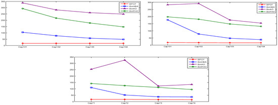
Figure 10.
The time results of BPO1 compared to other algorithms.
Figure 10 shows that the computational time results for BPO1 remain at very low levels across all datasets and are presented as an almost flat line. This demonstrates that BPO1 is highly efficient and consistent in terms of computational time. The algorithms BinEMA and BinFHO are reported to have achieved significantly higher time values. In the graphs, BinEMA is seen to have produced high and fluctuating time results in most datasets. BinFHO, although it produces lower values than BinEMA in some small datasets, is generally associated with high and unstable computational costs. In the datasets with 16, 20, and 24 items, the time values of BinEMA and BinFHO exhibit sharp increases and decreases, which are interpreted as unstable and costly computational behavior. In contrast, BPO1 is illustrated to follow a consistently low and stable line. As a result, the graphs clearly demonstrate that BPO1 is significantly faster than the other algorithms in terms of time and is proven to maintain its efficiency even as the problem scale increases. This confirms that BPO1 is not only superior in terms of solution quality but is also established as advantageous in terms of computational cost.
5.2. Experimental Results of BPO2 for UFLP
The UFLP is categorized based on its problem size and difficulty level, ranging from small to huge. This ensures a diverse and comprehensive evaluation of the optimization algorithm’s performance across varying problem complexities. Table 16 shows the BPO2 parameter values used in the experiments. A comprehensive dataset of 12 different UFLPs is available from the OR Library, as illustrated in Table 17. Table 18 reports the best values, Table 19 provides the standard deviation values indicating stability, Table 20 summarizes the mean value, Table 21 shows the GAP values reflecting proximity to the optimum, Table 22 presents the worst results, and Table 23 reports the computational time results, highlighting efficiency. These tables show the performance of the BPO2 algorithm under TF1-TF8 variants. In the tables, The bolded values indicate the optimum value.
Table 16.
BPO2′s parameter settings.
Table 16.
BPO2′s parameter settings.
| Parameters | Values |
|---|---|
| Population size (N) | 40 |
| Maximum iteration (MaxIter) | 2000 |
| MaxFEs | 80,000 |
| Number of runs | 30 |
Table 17.
Characteristics of the UFLP from the OR library.
Table 17.
Characteristics of the UFLP from the OR library.
| Problem Name | Difficulty Level Size | Size of the Problem | Optimum |
|---|---|---|---|
| Cap71 | Small | 16 × 50 | 9.3262 × 10⁵ |
| Cap72 | Small | 16 × 50 | 9.7780 × 10⁵ |
| Cap73 | Small | 16 × 50 | 1.01064 × 10⁶ |
| Cap74 | Small | 16 × 50 | 1.0350 × 10⁶ |
| Cap101 | Medium | 25 × 50 | 7.9664 × 10⁵ |
| Cap102 | Medium | 25 × 50 | 8.5470 × 10⁵ |
| Cap103 | Medium | 25 × 50 | 8.9378 × 10⁵ |
| Cap104 | Medium | 25 × 50 | 9.2894 × 10⁵ |
| Cap131 | Large | 50 × 50 | 7.9344 × 10⁵ |
| Cap132 | Large | 50 × 50 | 8.5150 × 10⁵ |
| Cap133 | Large | 50 × 50 | 8.9308 × 10⁵ |
| Cap134 | Large | 50 × 50 | 9.2894 × 10⁵ |
Table 18.
The statical best values of the BPO2.
Table 18.
The statical best values of the BPO2.
| Dataset | TF1-BPO2 | TF2-BPO2 | TF3-BPO2 | TF4-BPO2 | TF5-BPO2 | TF6-BPO2 | TF7-BPO2 | TF8-BPO2 |
|---|---|---|---|---|---|---|---|---|
| Cap71 | 9.3262 × 10⁵ | 9.3262 × 10⁵ | 9.3262 × 10⁵ | 9.3262 × 10⁵ | 9.3262 × 10⁵ | 9.4958 × 10⁵ | 9.3262 × 10⁵ | 9.3262 × 10⁵ |
| Cap72 | 9.7780 × 10⁵ | 9.8694 × 10⁵ | 9.7780 × 10⁵ | 9.7780 × 10⁵ | 9.7780 × 10⁵ | 9.7780 × 10⁵ | 9.7780 × 10⁵ | 9.7780 × 10⁵ |
| Cap73 | 1.0106 × 10⁶ | 1.0106 × 10⁶ | 1.0106 × 10⁶ | 1.0106 × 10⁶ | 1.0106 × 10⁶ | 1.0106 × 10⁶ | 1.0106 × 10⁶ | 1.0106 × 10⁶ |
| Cap74 | 1.0350 × 10⁶ | 1.0350 × 10⁶ | 1.0350 × 10⁶ | 1.0350 × 10⁶ | 1.0350 × 10⁶ | 1.0350 × 10⁶ | 1.0350 × 10⁶ | 1.0350 × 10⁶ |
| Cap101 | 7.9665 × 10⁵ | 7.9665 × 10⁵ | 7.9665 × 10⁵ | 7.9665 × 10⁵ | 7.9665 × 10⁵ | 7.9665 × 10⁵ | 7.9665 × 10⁵ | 7.9665 × 10⁵ |
| Cap102 | 8.5470 × 10⁵ | 8.5470 × 10⁵ | 8.5470 × 10⁵ | 8.5470 × 10⁵ | 8.5470 × 10⁵ | 8.5470 × 10⁵ | 8.5470 × 10⁵ | 8.5470 × 10⁵ |
| Cap103 | 8.9378 × 10⁵ | 8.9457 × 10⁵ | 8.9378 × 10⁵ | 8.9378 × 10⁵ | 8.9401 × 10⁵ | 8.9378 × 10⁵ | 8.9378 × 10⁵ | 8.9378 × 10⁵ |
| Cap104 | 9.2894 × 10⁵ | 9.2894 × 10⁵ | 9.2894 × 10⁵ | 9.2894 × 10⁵ | 9.2894 × 10⁵ | 9.2894 × 10⁵ | 9.2894 × 10⁵ | 9.2894 × 10⁵ |
| Cap131 | 7.9742 × 10⁵ | 8.0031 × 10⁵ | 7.9793 × 10⁵ | 8.0124 × 10⁵ | 7.9840 × 10⁵ | 8.0058 × 10⁵ | 7.9774 × 10⁵ | 8.0351 × 10⁵ |
| Cap132 | 8.5761 × 10⁵ | 8.5752 × 10⁵ | 8.5453 × 10⁵ | 8.5755 × 10⁵ | 8.6033 × 10⁵ | 8.5351 × 10⁵ | 8.5522 × 10⁵ | 8.5385 × 10⁵ |
| Cap133 | 8.9687 × 10⁵ | 8.9920 × 10⁵ | 8.9927 × 10⁵ | 8.9480 × 10⁵ | 8.9559 × 10⁵ | 8.9723 × 10⁵ | 8.9568 × 10⁵ | 8.9475 × 10⁵ |
| Cap134 | 9.3151 × 10⁵ | 9.2894 × 10⁵ | 9.2894 × 10⁵ | 9.2894 × 10⁵ | 9.2948 × 10⁵ | 9.2948 × 10⁵ | 9.2948 × 10⁵ | 9.2948 × 10⁵ |
| Total Rank | 1.0914 × 10⁷ | 1.0926 × 10⁷ | 1.0911 × 10⁷ | 1.0913 × 10⁷ | 1.0914 × 10⁷ | 1.0928 × 10⁷ | 1.0908 × 10⁷ | 1.0912 × 10⁷ |
| Finally Rank | 5 | 7 | 2 | 4 | 5 | 8 | 1 | 3 |
In Table 18, the Total Rank row represents the overall performance of each TF across all datasets. The lowest total value, 1.0908 × 10⁷, is obtained by TF7, demonstrating that TF7 has provided the best overall performance. The Finally Rank row summarizes the ranking of these total values. TF7 is placed first (rank = 1), followed by TF3 in second (rank = 2), TF8 in third (rank = 3), and TF4 in fourth (rank = 4).
Table 19.
The statical standard deviation results of the BPO2.
Table 19.
The statical standard deviation results of the BPO2.
| Dataset | TF1-BPO2 | TF2-BPO2 | TF3-BPO2 | TF4-BPO2 | TF5-BPO2 | TF6-BPO2 | TF7-BPO2 | TF8-BPO2 |
|---|---|---|---|---|---|---|---|---|
| Cap71 | 0 | 0 | 0 | 0 | 0 | 0 | 0 | 0 |
| Cap72 | 0 | 0 | 0 | 0 | 0 | 0 | 0 | 0 |
| Cap73 | 0 | 0 | 0 | 0 | 0 | 0 | 0 | 0 |
| Cap74 | 0 | 0 | 0 | 0 | 0 | 0 | 0 | 0 |
| Cap101 | 0 | 0 | 0 | 0 | 0 | 0 | 0 | 0 |
| Cap102 | 0 | 0 | 0 | 0 | 0 | 0 | 0 | 0 |
| Cap103 | 0 | 0 | 0 | 0 | 0 | 0 | 0 | 0 |
| Cap104 | 0 | 0 | 0 | 0 | 0 | 0 | 0 | 0 |
| Cap131 | 0 | 0 | 0 | 0 | 0 | 0 | 0 | 0 |
| Cap132 | 0 | 0 | 0 | 0 | 0 | 0 | 0 | 0 |
| Cap133 | 0 | 0 | 0 | 0 | 0 | 0 | 0 | 0 |
| Cap134 | 0 | 0 | 0 | 0 | 0 | 0 | 0 | 0 |
| Total Rank | 0 | 0 | 0 | 0 | 0 | 0 | 0 | 0 |
| Finally Rank | 1 | 1 | 1 | 1 | 1 | 1 | 1 | 1 |
Table 19 presents the standard deviation results of BPO2 across different TFs (TF1-TF8) for the UFLP. It is observed that the standard deviation values are consistently recorded as zero for all datasets and all TFs, indicating that the algorithm has produced identical results in every independent run. Consequently, the Total Rank values are also zero across all TFs, and the Finally Rank row assigns all TFs the first rank (rank = 1). These outcomes demonstrate that BPO2 exhibits perfect stability and robustness on the tested datasets, ensuring that no variability is observed across runs regardless of the TFs employed.
Table 20.
The mean results of the BPO2.
Table 20.
The mean results of the BPO2.
| Dataset | TF1-BPO2 | TF2-BPO2 | TF3-BPO2 | TF4-BPO2 | TF5-BPO2 | TF6-BPO2 | TF7-BPO2 | TF8-BPO2 |
|---|---|---|---|---|---|---|---|---|
| Cap71 | 9.3262 × 10⁵ | 9.3262 × 10⁵ | 9.3262 × 10⁵ | 9.3262 × 10⁵ | 9.3262 × 10⁵ | 9.4958 × 10⁵ | 9.3262 × 10⁵ | 9.3262 × 10⁵ |
| Cap72 | 9.7780 × 10⁵ | 9.8694 × 10⁵ | 9.7780 × 10⁵ | 9.7780 × 10⁵ | 9.7780 × 10⁵ | 9.7780 × 10⁵ | 9.7780 × 10⁵ | 9.7780 × 10⁵ |
| Cap73 | 1.0106 × 10⁶ | 1.0106 × 10⁶ | 1.0106 × 10⁶ | 1.0106 × 10⁶ | 1.0106 × 10⁶ | 1.0106 × 10⁶ | 1.0106 × 10⁶ | 1.0106 × 10⁶ |
| Cap74 | 1.0350 × 10⁶ | 1.0350 × 10⁶ | 1.0350 × 10⁶ | 1.0350 × 10⁶ | 1.0350 × 10⁶ | 1.0350 × 10⁶ | 1.0350 × 10⁶ | 1.0350 × 10⁶ |
| Cap101 | 7.9665 × 10⁵ | 7.9665 × 10⁵ | 7.9665 × 10⁵ | 7.9665 × 10⁵ | 7.9665 × 10⁵ | 7.9665 × 10⁵ | 7.9665 × 10⁵ | 7.9665 × 10⁵ |
| Cap102 | 8.5470 × 10⁵ | 8.5470 × 10⁵ | 8.5470 × 10⁵ | 8.5470 × 10⁵ | 8.5470 × 10⁵ | 8.5470 × 10⁵ | 8.5470 × 10⁵ | 8.5470 × 10⁵ |
| Cap103 | 8.9378 × 10⁵ | 8.9457 × 10⁵ | 8.9378 × 10⁵ | 8.9378 × 10⁵ | 8.9401 × 10⁵ | 8.9378 × 10⁵ | 8.9378 × 10⁵ | 8.9378 × 10⁵ |
| Cap104 | 9.2894 × 10⁵ | 9.2894 × 10⁵ | 9.2894 × 10⁵ | 9.2894 × 10⁵ | 9.2894 × 10⁵ | 9.2894 × 10⁵ | 9.2894 × 10⁵ | 9.2894 × 10⁵ |
| Cap131 | 7.9742 × 10⁵ | 8.0031 × 10⁵ | 7.9793 × 10⁵ | 8.0124 × 10⁵ | 7.9840 × 10⁵ | 8.0058 × 10⁵ | 7.9774 × 10⁵ | 8.0351 × 10⁵ |
| Cap132 | 8.5761 × 10⁵ | 8.5752 × 10⁵ | 8.5453 × 10⁵ | 8.5755 × 10⁵ | 8.6033 × 10⁵ | 8.5351 × 10⁵ | 8.5522 × 10⁵ | 8.5385 × 10⁵ |
| Cap133 | 8.9687 × 10⁵ | 8.9920 × 10⁵ | 8.9927 × 10⁵ | 8.9480 × 10⁵ | 8.9559 × 10⁵ | 8.9723 × 10⁵ | 8.9568 × 10⁵ | 8.9475 × 10⁵ |
| Cap134 | 9.3151 × 10⁵ | 9.2894 × 10⁵ | 9.2894 × 10⁵ | 9.2894 × 10⁵ | 9.2948 × 10⁵ | 9.2948 × 10⁵ | 9.2948 × 10⁵ | 9.2948 × 10⁵ |
| Total Rank | 1.0914 × 10⁷ | 1.0926 × 10⁷ | 1.0911 × 10⁷ | 1.0913 × 10⁷ | 1.0914 × 10⁷ | 1.0928 × 10⁷ | 1.0908 × 10⁷ | 1.0912 × 10⁷ |
| Finally Rank | 5 | 7 | 2 | 4 | 5 | 8 | 1 | 3 |
Table 20 shows mean results indicate that although all TFs provide competitive outcomes, certain TFs yield slight advantages in specific datasets. The Total Rank values reinforce this, with TF7 obtaining the lowest cumulative score (rank = 1), followed by TF3 (rank = 2), TF8 (rank = 3), and TF4 (rank = 4). The Finally Rank row, therefore, highlights TF7 as the most effective TFs overall, combining consistency with competitiveness, while the remaining TFs also deliver reliable performance with dataset-specific strengths.
Table 21.
The statical GAP values of the BPO2.
Table 21.
The statical GAP values of the BPO2.
| Dataset | TF1-BPO2 | TF2-BPO2 | TF3-BPO2 | TF4-BPO2 | TF5-BPO2 | TF6-BPO2 | TF7-BPO2 | TF8-BPO2 |
|---|---|---|---|---|---|---|---|---|
| Cap71 | 0 | 0 | 0 | 0 | 0 | 1.8185 × 100 | 0 | 0 |
| Cap72 | 0 | 9.3491 × 10⁻¹ | 0 | 0 | 0 | 0 | 0 | 0 |
| Cap73 | 0 | 0 | 0 | 0 | 0 | 0 | 0 | 0 |
| Cap74 | 0 | 0 | 0 | 0 | 0 | 0 | 0 | 0 |
| Cap101 | 1.4613 × 10⁻¹⁴ | 1.4613 × 10⁻¹⁴ | 1.4613 × 10⁻¹⁴ | 1.4613 × 10⁻¹⁴ | 1.4613 × 10⁻¹⁴ | 1.4613 × 10⁻¹⁴ | 1.4613 × 10⁻¹⁴ | 1.4613 × 10⁻¹⁴ |
| Cap102 | 1.3621 × 10⁻¹⁴ | 1.3621 × 10⁻¹⁴ | 1.3621 × 10⁻¹⁴ | 1.3621 × 10⁻¹⁴ | 1.3621 × 10⁻¹⁴ | 1.3621 × 10⁻¹⁴ | 1.3621 × 10⁻¹⁴ | 1.3621 × 10⁻¹⁴ |
| Cap103 | 0 | 8.8567 × 10⁻² | 0 | 0 | 2.5289 × 10⁻² | 0 | 0 | 0 |
| Cap104 | 1.2532 × 10⁻¹⁴ | 1.2532 × 10⁻¹⁴ | 1.2532 × 10⁻¹⁴ | 1.2532 × 10⁻¹⁴ | 1.2532 × 10⁻¹⁴ | 1.2532 × 10⁻¹⁴ | 1.2532 × 10⁻¹⁴ | 1.2532 × 10⁻¹⁴ |
| Cap131 | 5.0167 × 10⁻¹ | 8.6586 × 10⁻¹ | 5.6634 × 10⁻¹ | 9.8266 × 10⁻¹ | 6.2559 × 10⁻¹ | 8.9979 × 10⁻¹ | 5.4144 × 10⁻¹ | 1.2694 × 100 |
| Cap132 | 7.1793 × 10⁻¹ | 7.0697 × 10⁻¹ | 3.5643 × 10⁻¹ | 7.1090 × 10⁻¹ | 1.0374 × 100 | 2.3665 × 10⁻¹ | 4.3702 × 10⁻¹ | 2.7668 × 10⁻¹ |
| Cap133 | 4.2463 × 10⁻¹ | 6.8536 × 10⁻¹ | 6.9381 × 10⁻¹ | 1.9309 × 10⁻¹ | 2.8173 × 10⁻¹ | 4.6505 × 10⁻¹ | 2.9188 × 10⁻¹ | 1.8759 × 10⁻¹ |
| Cap134 | 2.7621 × 10⁻¹ | 1.2532 × 10⁻¹⁴ | 5.7680 × 10⁻² | 1.2532 × 10⁻¹⁴ | 1.2532 × 10⁻¹⁴ | 5.7680 × 10⁻² | 5.7680 × 10⁻² | 5.7680 × 10⁻² |
| Total Rank | 1.9184 × 100 | 3.2817 × 100 | 1.6739 × 100 | 1.8867 × 100 | 1.9700 × 100 | 3.4777 × 100 | 1.3280 × 100 | 1.7914 × 100 |
| Finally Rank | 5 | 7 | 2 | 4 | 6 | 8 | 1 | 3 |
Table 21 shows the GAP values, where certain TFs exhibit slight advantages on certain datasets. The overall Ranking values highlight these differences; TF7 achieves the lowest cumulative GAP score (rank = 1), followed by TF3 (rank = 2), TF8 (rank = 3), and TF4 (rank = 4). Consequently, the final Ranking line identifies TF7 as the most effective TFs overall because it combines robustness with accuracy.
Table 22.
The statical worst results of the BPO2.
Table 22.
The statical worst results of the BPO2.
| Dataset | TF1-BPO2 | TF2-BPO2 | TF3-BPO2 | TF4-BPO2 | TF5-BPO2 | TF6-BPO2 | TF7-BPO2 | TF8-BPO2 |
|---|---|---|---|---|---|---|---|---|
| Cap71 | 9.3262 × 10⁵ | 9.3262 × 10⁵ | 9.3262 × 10⁵ | 9.3262 × 10⁵ | 9.3262 × 10⁵ | 9.4958 × 10⁵ | 9.3262 × 10⁵ | 9.3262 × 10⁵ |
| Cap72 | 9.7780 × 10⁵ | 9.8694 × 10⁵ | 9.7780 × 10⁵ | 9.7780 × 10⁵ | 9.7780 × 10⁵ | 9.7780 × 10⁵ | 9.7780 × 10⁵ | 9.7780 × 10⁵ |
| Cap73 | 1.0106 × 10⁶ | 1.0106 × 10⁶ | 1.0106 × 10⁶ | 1.0106 × 10⁶ | 1.0106 × 10⁶ | 1.0106 × 10⁶ | 1.0106 × 10⁶ | 1.0106 × 10⁶ |
| Cap74 | 1.0350 × 10⁶ | 1.0350 × 10⁶ | 1.0350 × 10⁶ | 1.0350 × 10⁶ | 1.0350 × 10⁶ | 1.0350 × 10⁶ | 1.0350 × 10⁶ | 1.0350 × 10⁶ |
| Cap101 | 7.9665 × 10⁵ | 7.9665 × 10⁵ | 7.9665 × 10⁵ | 7.9665 × 10⁵ | 7.9665 × 10⁵ | 7.9665 × 10⁵ | 7.9665 × 10⁵ | 7.9665 × 10⁵ |
| Cap102 | 8.5470 × 10⁵ | 8.5470 × 10⁵ | 8.5470 × 10⁵ | 8.5470 × 10⁵ | 8.5470 × 10⁵ | 8.5470 × 10⁵ | 8.5470 × 10⁵ | 8.5470 × 10⁵ |
| Cap103 | 8.9378 × 10⁵ | 8.9457 × 10⁵ | 8.9378 × 10⁵ | 8.9378 × 10⁵ | 8.9401 × 10⁵ | 8.9378 × 10⁵ | 8.9378 × 10⁵ | 8.9378 × 10⁵ |
| Cap104 | 9.2894 × 10⁵ | 9.2894 × 10⁵ | 9.2894 × 10⁵ | 9.2894 × 10⁵ | 9.2894 × 10⁵ | 9.2894 × 10⁵ | 9.2894 × 10⁵ | 9.2894 × 10⁵ |
| Cap131 | 7.9742 × 10⁵ | 8.0031 × 10⁵ | 7.9793 × 10⁵ | 8.0124 × 10⁵ | 7.9840 × 10⁵ | 8.0058 × 10⁵ | 7.9774 × 10⁵ | 8.0351 × 10⁵ |
| Cap132 | 8.5761 × 10⁵ | 8.5752 × 10⁵ | 8.5453 × 10⁵ | 8.5755 × 10⁵ | 8.6033 × 10⁵ | 8.5351 × 10⁵ | 8.5522 × 10⁵ | 8.5385 × 10⁵ |
| Cap133 | 8.9687 × 10⁵ | 8.9920 × 10⁵ | 8.9927 × 10⁵ | 8.9480 × 10⁵ | 8.9559 × 10⁵ | 8.9723 × 10⁵ | 8.9568 × 10⁵ | 8.9475 × 10⁵ |
| Cap134 | 9.3151 × 10⁵ | 9.2894 × 10⁵ | 9.2894 × 10⁵ | 9.2894 × 10⁵ | 9.2948 × 10⁵ | 9.2948 × 10⁵ | 9.2948 × 10⁵ | 9.2948 × 10⁵ |
| Total Rank | 1.0914 × 10⁷ | 1.0926 × 10⁷ | 1.0911 × 10⁷ | 1.0913 × 10⁷ | 1.0914 × 10⁷ | 1.0928 × 10⁷ | 1.0908 × 10⁷ | 1.0912 × 10⁷ |
| Finally Rank | 5 | 7 | 2 | 4 | 5 | 8 | 1 | 3 |
Table 22 presents the worst results of BPO2 across the UFLP using eight different TFs (TF1-TF8). The Finally Rank row highlights TF7 as the best-performing TF in terms of worst results (rank = 1), showcasing its robustness and reliability, with TF3 (rank = 2) and TF8 (rank = 3) emerging as competitive alternatives.
Table 23.
The statical time results of the BPO2.
Table 23.
The statical time results of the BPO2.
| Dataset | TF1-BPO2 | TF2-BPO2 | TF3-BPO2 | TF4-BPO2 | TF5-BPO2 | TF6-BPO2 | TF7-BPO2 | TF8-BPO2 |
|---|---|---|---|---|---|---|---|---|
| Cap71 | 1.7468 × 101 | 1.7116 × 101 | 1.6772 × 101 | 1.6913 × 101 | 1.7519 × 101 | 1.7613 × 101 | 1.6903 × 101 | 1.7287 × 101 |
| Cap72 | 1.6622 × 101 | 1.6908 × 101 | 1.6567 × 101 | 1.6847 × 101 | 1.7206 × 101 | 1.6635 × 101 | 1.6571 × 101 | 1.6660 × 101 |
| Cap73 | 1.6441 × 101 | 1.6557 × 101 | 1.6392 × 101 | 1.6328 × 101 | 1.6988 × 101 | 1.6403 × 101 | 1.5571 × 101 | 1.5577 × 101 |
| Cap74 | 1.5355 × 101 | 1.5582 × 101 | 1.5426 × 101 | 1.5424 × 101 | 1.5769 × 101 | 1.5379 × 101 | 1.5271 × 101 | 1.5326 × 101 |
| Cap101 | 1.7894 × 101 | 1.7813 × 101 | 1.7897 × 101 | 1.7471 × 101 | 1.8207 × 101 | 1.7757 × 101 | 1.7825 × 101 | 1.7624 × 101 |
| Cap102 | 1.7309 × 101 | 1.7142 × 101 | 1.7241 × 101 | 1.7193 × 101 | 1.7928 × 101 | 1.7429 × 101 | 1.7258 × 101 | 1.7339 × 101 |
| Cap103 | 1.7007 × 101 | 1.7084 × 101 | 1.7291 × 101 | 1.7021 × 101 | 1.7876 × 101 | 1.6273 × 101 | 1.5989 × 101 | 1.6092 × 101 |
| Cap104 | 1.6057 × 101 | 1.5991 × 101 | 1.6095 × 101 | 1.6019 × 101 | 1.6472 × 101 | 1.5888 × 101 | 1.5921 × 101 | 1.5910 × 101 |
| Cap131 | 1.7221 × 101 | 1.7612 × 101 | 1.6910 × 101 | 1.6905 × 101 | 1.7882 × 101 | 1.7015 × 101 | 1.6892 × 101 | 1.6919 × 101 |
| Cap132 | 1.6728 × 101 | 1.6731 × 101 | 1.6739 × 101 | 1.6743 × 101 | 1.7667 × 101 | 1.6773 × 101 | 1.6730 × 101 | 1.6761 × 101 |
| Cap133 | 1.6660 × 101 | 1.6666 × 101 | 1.6665 × 101 | 1.6665 × 101 | 1.7601 × 101 | 1.6692 × 101 | 1.6654 × 101 | 1.6695 × 101 |
| Cap134 | 1.6627 × 101 | 1.6621 × 101 | 1.6633 × 101 | 1.6647 × 101 | 1.7576 × 101 | 1.6656 × 101 | 1.6626 × 101 | 1.6655 × 101 |
| Total Rank | 2.0139 × 10² | 2.0182 × 10² | 2.0063 × 10² | 2.0018 × 10² | 2.0869 × 10² | 2.0051 × 10² | 1.9821 × 10² | 1.9884 × 10² |
| Finally Rank | 6 | 7 | 5 | 3 | 8 | 4 | 1 | 2 |
Table 23 shows the time performance of BPO2 with different transfer functions. All TFs achieve similar execution times, confirming the algorithm’s efficiency. TF7 records the lowest cumulative time (rank = 1), followed by TF8 (rank = 2) and TF4 (rank = 3), while TF5 has the highest (rank = 8), making TF7 the most efficient option overall.
The Wilcoxon signed-rank test is employed to determine whether there is a statistically significant difference between the performance distributions of the two algorithms. In the table, the symbol (+) indicates that a significant difference exists in favor of the proposed algorithm (p < 0.05). In contrast, the symbol (-) indicates that no statistically significant difference is observed (p ≥ 0.05). This analysis provides a clear statistical validation of the similarities and differences among the algorithms under comparison [61].
Table 24 presents the results of the Wilcoxon signed-rank test conducted between the BPO2 and its variants using different TFs (i.e., TF1-BPO2 via TF2-BPO2, TF2-BPO2 via TF3-BPO2, …, TF6-BPO2 via TF7-BPO2, TF7-BPO2 via TF8-BPO2). The results of Table 24 show that in the majority of cases, p-values are extremely small (close to zero) and h = +, confirming significant performance differences between TFs. Overall, these outcomes demonstrate that TFs’ selection significantly affects BPO2′s performance, with most TFs exhibiting statistically distinguishable results across datasets.
Table 24.
Wilcoxon signed-rank test results for BPO2 with different TFs.
Table 25 presents a comparison of BPO2-TF7 with three competing binary optimization algorithms: Binary Honey Badger Algorithm (BinHBA), Binary Aquila Optimizer (BinAO), and Binary Fire Hawk Optimizer (BinFHO) in terms of standard deviation on the UFLP datasets. The results of BinHBA, BinAO, and BinFHO are taken from the literature [60]. All compared algorithms are executed under the same parameter settings as in Table 16.
Table 25.
Standard deviations results for BPO2 and other algorithms.
Table 25 shows that BPO2 consistently records a standard deviation of 0 in all datasets, indicating that BPO2 has produced identical results across all independent runs. These findings demonstrate that BPO2 is the most stable and reliable algorithm in terms of robustness. In contrast, the results of BinHBA, BinAO, and BinFHO exhibit considerable fluctuations and inconsistencies. Table 26 reports the GAP values for BPO2 and the competing other algorithms on the UFLP.
Table 26.
GAP values for BPO2 and other algorithms.
In Table 26, TF7-BPO2 consistently achieves values equal to zero or very close to zero across nearly all instances, indicating that the obtained solutions are highly proximate to the known optima. By contrast, BinHBA, BinAO, and BinFHO generate considerably higher GAP values, particularly in larger and more challenging datasets such as Cap131-Cap133. These findings clearly demonstrate that TF7-BPO2 provides superior accuracy and reliability compared to the competing algorithms. Table 27 reports the execution times of BPO2 and the competing algorithms on the UFLP datasets.
Table 27.
Running times of BPO2 and other algorithms.
In Table 27, TF7-BPO2 consistently achieves execution times in the narrow range of approximately 15–18 seconds across all datasets, demonstrating remarkable efficiency and stability. In contrast, the competing algorithms require substantially higher times, often exceeding 100 seconds, with BinAO in particular reaching over 300 seconds in larger instances such as Cap131-Cap133. These sharp differences highlight that TF7-BPO2 is not only the fastest algorithm but also the most consistent in terms of runtime performance. While BinHBA, BinAO, and BinFHO exhibit significant variability and scalability issues as the dataset size increases, TF7-BPO2 maintains nearly constant computational costs regardless of problem complexity. This stability ensures that the algorithm remains efficient and scalable, making it highly suitable for large-scale UFLP instances where both solution quality and computational efficiency are critical.
Figure 11 shows the computation times of TF7-BPO2 compared to BinHBA, BinAO, and BinFHO. While BPO2 consistently maintains low and stable execution costs even as the problem scale increases, the other algorithms exhibit substantially higher times accompanied by considerable fluctuations. This result highlights the superior efficiency and robustness of BPO2 in handling larger and more complex instances.
Figure 11.
The time results of BPO2 compared to other algorithms.
6. Conclusions
A novel binary metaheuristic, the Binary Puma Optimizer (BPO), is proposed in this study. In BPO, the original Puma Optimizer are transformed into the binary domain through eight transfer functions (four S-shaped and four V-shaped). Two problem-specific variants are proposed: BPO1, designed to address the 0-1 Knapsack Problems (KPs), and BPO2, developed for the unconstrained Uncapacitated Facility Location Problem (UFLP). In the 0-1 KP experiments, TF4 is identified as the most effective transfer function for BPO1. In contrast, the UFLP experiments demonstrate complete stability (zero standard deviation) across all transfer functions, with TF7 achieving the best overall performance.
Through comparative analyses, the competitiveness of the proposed approach is further demonstrated. Under identical experimental settings for KPs, BPO1-TF4 is consistently shown to outperform The Binary Evolutionary Mating Algorithm (BinEMA), the Binary Fire Hawk Optimizer (BinFHO), and S-shape Binary Whale Optimization Algorithm (BWOS) in terms of solution quality, robustness, and runtime. For the UFLP, significant success is achieved by BPO2-TF7, particularly over Binary Honey Badger Algorithm (BinHBA), Binary Aquila Optimizer (BinAO), and Binary Fire Hawk Optimizer (BinFHO) in terms of GAP values and computational time rankings.
Overall, the BPO can be regarded as a robust and versatile framework that not only ensures high accuracy and stability but also establishes a promising benchmark for future study in binary optimization algorithms.
Future study will focus on several promising directions: (i) designing adaptive and ensemble strategies for transfer function selection or switching; (ii) extending BPO to broader application domains, including feature selection, and multi-objective optimization; (iii) conducting comprehensive parameter tuning and ablation studies; (iv) incorporating advanced local search procedures.
Author Contributions
A.I.: conceptualization, formal analysis, investigation, methodology, software, visualization, and writing—original draft preparation. T.S.: methodology, formal analysis, investigation, software, review and editing, and supervision. All authors have read and agreed to the published version of the manuscript.
Funding
This study received no external funding.
Data Availability Statement
The original contributions presented in this study are included in the article. Further inquiries can be directed at the corresponding author.
Acknowledgments
This study is derived from a part of Aysegul Ihsan’s doctoral dissertation at Selcuk University. The authors would like to thank the project for using the laboratory facilities supported by the “Data Intensive and Computational Vision Research Laboratory Infrastructure Project” (BAP project number 20301027) in this research.
Conflicts of Interest
The authors declare no conflicts of interest.
References
- Probert, M. Engineering Optimisation: An Introduction with Metaheuristic Applications, by Xin-She Yang. Contemp. Phys. 2012, 53, 271–272. [Google Scholar] [CrossRef]
- Mirjalili, S.; Lewis, A. S-shaped versus V-shaped transfer functions for binary Particle Swarm Optimization. Swarm Evol. Comput. 2013, 9, 1–14. [Google Scholar] [CrossRef]
- Franken, N.; Engelbrecht, A.P. Particle swarm optimization approaches to coevolve strategies for the iterated prisoner’s dilemma. IEEE Trans. Evol. Comput. 2005, 9, 562–579. [Google Scholar] [CrossRef]
- Alawad, N.A.; Abed-alguni, B.H.; Al-Betar, M.A.; Jaradat, A. Binary improved white shark algorithm for intrusion detection systems. Neural Comput. Appl. 2023, 35, 19427–19451. [Google Scholar] [CrossRef]
- Abdollahzadeh, B.; Khodadadi, N.; Barshandeh, S.; Trojovsky, P.; Soleimanian Gharehchopogh, F.; El-kenawy, E.-S.; Abualigah, L.; Mirjalili, S. Puma optimizer (PO): A novel metaheuristic optimization algorithm and its application in machine learning. Clust. Comput. 2024, 27, 5235–5283. [Google Scholar] [CrossRef]
- Keleş, M.K.; Kiliç, Ü. Binary Black Widow Optimization Approach for Feature Selection. IEEE Access 2022, 10, 95936–95948. [Google Scholar] [CrossRef]
- Khishe, M.; Mosavi, M.R. Chimp optimization algorithm. Expert Syst. Appl. 2020, 149, 113338. [Google Scholar] [CrossRef]
- Wang, J.; Khishe, M.; Kaveh, M.; Mohammadi, H. Binary Chimp Optimization Algorithm (BChOA): A New Binary Meta-heuristic for Solving Optimization Problems. Cogn. Comput. 2021, 13, 1297–1316. [Google Scholar] [CrossRef]
- Li, S.; Chen, H.; Wang, M.; Heidari, A.A.; Mirjalili, S. Slime mould algorithm: A new method for stochastic optimization. Future Gener. Comput. Syst. 2020, 111, 300–323. [Google Scholar] [CrossRef]
- Abdel-Basset, M.; Mohamed, R.; Chakrabortty, R.K.; Ryan, M.J.; Mirjalili, S. An efficient binary slime mould algorithm integrated with a novel attacking-feeding strategy for feature selection. Comput. Ind. Eng. 2021, 153, 107078. [Google Scholar] [CrossRef]
- Agushaka, J.O.; Ezugwu, A.E.; Abualigah, L. Dwarf Mongoose Optimization Algorithm. Comput. Methods Appl. Mech. Eng. 2022, 391, 114570. [Google Scholar] [CrossRef]
- Akinola, O.A.; Agushaka, J.O.; Ezugwu, A.E. Binary dwarf mongoose optimizer for solving high-dimensional feature selection problems. PLoS ONE 2022, 17, e0274850. [Google Scholar] [CrossRef]
- Oyelade, O.N.; Ezugwu, A.E.S.; Mohamed, T.I.A.; Abualigah, L. Ebola Optimization Search Algorithm: A New Nature-Inspired Metaheuristic Optimization Algorithm. IEEE Access 2022, 10, 16150–16177. [Google Scholar] [CrossRef]
- Abualigah, L.; Diabat, A.; Mirjalili, S.; Abd Elaziz, M.; Gandomi, A.H. The Arithmetic Optimization Algorithm. Comput. Methods Appl. Mech. Eng. 2021, 376, 113609. [Google Scholar] [CrossRef]
- Xu, M.; Song, Q.; Xi, M.; Zhou, Z. Binary arithmetic optimization algorithm for feature selection. Soft Comput. 2023, 27, 11395–11429. [Google Scholar] [CrossRef] [PubMed]
- Yildizdan, G.; Baş, E. A Novel Binary Artificial Jellyfish Search Algorithm for Solving 0–1 Knapsack Problems. Neural Process. Lett. 2023, 55, 8605–8671. [Google Scholar] [CrossRef]
- Akinola, O.; Oyelade, O.N.; Ezugwu, A.E. Binary Ebola optimization search algorithm for feature selection and classification problems. Appl. Sci. 2022, 12, 11787. [Google Scholar] [CrossRef]
- Yang, Y.; Chen, H.; Heidari, A.A.; Gandomi, A.H. Hunger games search: Visions, conception, implementation, deep analysis, perspectives, and towards performance shifts. Expert Syst. Appl. 2021, 177, 114864. [Google Scholar] [CrossRef]
- Devi, R.; Manoharan, P.; Jangir, P.; Kumar, D.; Alrowaili, D.; Nisar, K. BHGSO: Binary Hunger Games Search Optimization Algorithm for Feature Selection Problem. CMC Tech Sci. Press 2021, 70, 557–579. [Google Scholar] [CrossRef]
- Baş, E. Binary Aquila Optimizer for 0–1 knapsack problems. Eng. Appl. Artif. Intell. 2023, 118, 105592. [Google Scholar] [CrossRef]
- Mohammadzadeh, A.; Masdari, M.; Gharehchopogh, F.S.; Jafarian, A. Improved chaotic binary grey wolf optimization algorithm for workflow scheduling in green cloud computing. Evol. Intell. 2021, 14, 1997–2025. [Google Scholar] [CrossRef]
- Seyyedabbasi, A.; Hu, G.; Shehadeh, H.; Wang, X.; Canatalay, P. V-shaped and S-shaped binary artificial protozoa optimizer (APO) algorithm for wrapper feature selection on biological data. Clust. Comput. 2025, 28, 163. [Google Scholar] [CrossRef]
- Li, M.; Luo, Q.; Zhou, Y. BGOA-TVG: Binary Grasshopper Optimization Algorithm with Time-Varying Gaussian Transfer Functions for Feature Selection. Biomimetics 2024, 9, 187. [Google Scholar] [CrossRef]
- Sharma, R.; Mahanti, G.K.; Panda, G.; Rath, A.; Dash, S.; Mallik, S.; Zhao, Z. Comparative performance analysis of binary variants of FOX optimization algorithm with half-quadratic ensemble ranking method for thyroid cancer detection. Sci. Rep. 2023, 13, 19598. [Google Scholar] [CrossRef]
- Hassan, I.H.; Abdullahi, M.; Aliyu, M.M.; Yusuf, S.A.; Abdulrahim, A. An improved binary manta ray foraging optimization algorithm based feature selection and random forest classifier for network intrusion detection. Intell. Syst. Appl. 2022, 16, 200114. [Google Scholar] [CrossRef]
- Balakrishnan, K.; Dhanalakshmi, R.; Seetharaman, G. S-shaped and V-shaped binary African vulture optimization algorithm for feature selection. Expert Syst. 2022, 39, e13079. [Google Scholar] [CrossRef]
- Sharafi, Y.; Teshnehlab, M. Opposition-based binary competitive optimization algorithm using time-varying V-shape transfer function for feature selection. Neural Comput. Appl. 2021, 33, 17497–17533. [Google Scholar] [CrossRef]
- Hussien, A.G.; Hassanien, A.E.; Houssein, E.H.; Bhattacharyya, S.; Amin, M. S-shaped Binary Whale Optimization Algorithm for Feature Selection. In Recent Trends in Signal and Image Processing; Bhattacharyya, S., Mukherjee, A., Bhaumik, H., Das, S., Yoshida, K., Eds.; Springer: Singapore, 2019; pp. 79–87. [Google Scholar]
- Gao, Y.; Zhang, F.; Zhao, Y.; Li, C. Quantum-Inspired Wolf Pack Algorithm to Solve the 0–1 Knapsack Problem. Math. Probl. Eng. 2018, 2018, 1–10. [Google Scholar] [CrossRef]
- Zouache, D.; Nouioua, F.; Moussaoui, A. Quantum-inspired firefly algorithm with particle swarm optimization for discrete optimization problems. Soft Comput. 2016, 20, 2781–2799. [Google Scholar] [CrossRef]
- Kulkarni, A.J.; Krishnasamy, G.; Abraham, A. Solution to 0–1 Knapsack Problem Using Cohort Intelligence Algorithm. In Cohort Intelligence: A Socio-Inspired Optimization Method; Kulkarni, A.J., Krishnasamy, G., Abraham, A., Eds.; Springer International Publishing: Cham, Switzerland, 2017; pp. 55–74. [Google Scholar]
- Erdoğan, F.; Karakoyun, M.; Gülcü, Ş. An effective binary dynamic grey wolf optimization algorithm for the 0–1 knapsack problem. Multimed. Tools Appl. 2024, 84, 23279–23311. [Google Scholar] [CrossRef]
- Abdel-Basset, M.; Mohamed, R.; Mirjalili, S. A binary equilibrium optimization algorithm for 0–1 knapsack problems. Comput. Ind. Eng. 2021, 151, 106946. [Google Scholar] [CrossRef]
- Yuan, J.; Li, Y. Solving binary multi-objective knapsack problems with novel greedy strategy. Memetic Comput. 2021, 13, 447–458. [Google Scholar] [CrossRef]
- Bansal, J.C.; Deep, K. A modified binary particle swarm optimization for knapsack problems. Appl. Math. Comput. 2012, 218, 11042–11061. [Google Scholar] [CrossRef]
- Rodrigues, D.; Yang, X.-S.; De Souza, A.N.; Papa, J.P. Binary flower pollination algorithm and its application to feature selection. In Recent Advances in Swarm Intelligence and Evolutionary Computation; Springer: Berlin/Heidelberg, Germany, 2014; pp. 85–100. [Google Scholar]
- Abdel-Basset, M.; El-Shahat, D.; El-Henawy, I. Solving 0–1 knapsack problem by binary flower pollination algorithm. Neural Comput. Appl. 2019, 31, 5477–5495. [Google Scholar] [CrossRef]
- Feng, Y.; Wang, G.-G.; Deb, S.; Lu, M.; Zhao, X.-J. Solving 0–1 knapsack problem by a novel binary monarch butterfly optimization. Neural Comput. Appl. 2017, 28, 1619–1634. [Google Scholar] [CrossRef]
- Mingo López, L.F.; Gómez Blas, N.; Arteta Albert, A. Multidimensional knapsack problem optimization using a binary particle swarm model with genetic operations. Soft Comput. 2018, 22, 2567–2582. [Google Scholar] [CrossRef]
- Kong, X.; Gao, L.; Ouyang, H.; Li, S. A simplified binary harmony search algorithm for large scale 0–1 knapsack problems. Expert Syst. Appl. 2015, 42, 5337–5355. [Google Scholar] [CrossRef]
- Kaya, E. BinGSO: Galactic swarm optimization powered by binary artificial algae algorithm for solving uncapacitated facility location problems. Neural Comput. Appl. 2022, 34, 11063–11082. [Google Scholar] [CrossRef]
- Sag, T.; Ihsan, A. Efficiency analysis of binary metaheuristic optimization algorithms for uncapacitated facility location problems. Appl. Soft Comput. 2025, 174, 112968. [Google Scholar] [CrossRef]
- Babalik, A.; Babadag, A. A binary grasshopper optimization algorithm for solving uncapacitated facility location problem. Eng. Sci. Technol. Int. J. 2025, 65, 102031. [Google Scholar] [CrossRef]
- Beşkirli, A. A Transfer Function-Based Binary Version of Improved Pied Kingfisher Optimizer for Solving the Uncapacitated Facility Location Problem. Biomimetics 2025, 10, 526. [Google Scholar] [CrossRef]
- Baş, E.; Yildizdan, G. A new binary arithmetic optimization algorithm for uncapacitated facility location problem. Neural Comput. Appl. 2023, 36, 4151–4177. [Google Scholar] [CrossRef]
- Kmich, M.; El Ghouate, N.; Bencharqui, A.; Karmouni, H.; Sayyouri, M.; Askar, S.S.; Abouhawwash, M. Chaotic Puma Optimizer Algorithm for controlling wheeled mobile robots. Eng. Sci. Technol. Int. J. 2025, 63, 101982. [Google Scholar] [CrossRef]
- Pravesjit, S.; Kantawong, K. Enhancing the Puma Optimizer Algorithm for Optimiza-tion Problems. In Proceedings of the 2025 Joint International Conference on Digital Arts, Media and Technology with ECTI Northern Section Conference on Electrical, Electronics, Computer and Telecommunications Engineering (ECTI DAMT & NCON), Nan, Thailand, 29 January–1 February 2025. [Google Scholar] [CrossRef]
- Esakkiappan, K.; Kandasamy, P.; Raja, R.; Rajendran, S.K. Improved Binary Quantum-Based Puma Opti-mizer for Optimal Location and Sizing of Micro Grid with Electric Vehicle Charging Station. Iran. J. Sci-Ence Technol. Trans. Electr. Eng. 2025. [Google Scholar] [CrossRef]
- Bas, E.; Guner, L.B. The binary crayfish optimization algorithm with bitwise operator and repair method for 0–1 knapsack problems: An improved model. Neural Comput. Appl. 2025, 37, 4733–4767. [Google Scholar] [CrossRef]
- Cornuéjols, G.; Nemhauser, G.; Wolsey, L. The Uncapicitated Facility Location Problem; Cornell University Operations Research and Industrial Engineering: Ithaca, NY, USA, 1983. [Google Scholar]
- Jakob, K.; Pruzan, P.M. The simple plant location problem: Survey and synthesis. Eur. J. Oper. Res. 1983, 12, 41. [Google Scholar] [CrossRef]
- Monabbati, E.; Kakhki, H.T. On a class of subadditive duals for the uncapacitated facility location problem. Appl. Math. Comput. 2015, 251, 118–131. [Google Scholar] [CrossRef]
- Aslan, M.; Gunduz, M.; Kiran, M.S. JayaX: Jaya algorithm with xor operator for binary optimization. Appl. Soft Comput. 2019, 82, 105576. [Google Scholar] [CrossRef]
- Kole, A.; Chakrabarti, P.; Bhattacharyya, S. An ant colony optimization algorithm for uncapacitated facility location problem. In Proceedings of the 38th International Conference on Computers and Industrial Engineering, Hong Kong, 16–18 October 2013. [Google Scholar]
- Siew Mooi, S.L.; Md Sultan, A.B.; Sulaiman, M.; Mustapha, A.; Leong, K.Y. Crossover and Mutation Operators of Genetic Algorithms. Int. J. Mach. Learn. Comput. 2017, 7, 9–12. [Google Scholar] [CrossRef]
- Kora, P.; Yadlapalli, P. Crossover Operators in Genetic Algorithms: A Review. Int. J. Comput. Appl. 2017, 162, 34–36. [Google Scholar] [CrossRef]
- Truong, T.K.; Li, K.; Xu, Y. Chemical reaction optimization with greedy strategy for the 0–1 knapsack problem. Appl. Soft Comput. 2013, 13, 1774–1780. [Google Scholar] [CrossRef]
- Lv, J.; Wang, X.; Huang, M.; Cheng, H.; Li, F. Solving 0–1 knapsack problem by greedy degree and expectation efficiency. Appl. Soft Comput. 2015, 41, 94–103. [Google Scholar] [CrossRef]
- Zhao, J.; Huang, T.; Pang, F.; Liu, Y. Genetic Algorithm Based on Greedy Strategy in the 0-1 Knapsack Problem. In Proceedings of the 2009 Third International Conference on Genetic and Evolutionary Computing, Guilin, China, 14–17 October 2009; pp. 105–107. [Google Scholar]
- Yildizdan, G.; Bas, E. A new binary coati optimization algorithm for binary optimization problems. Neural Comput. Appl. 2024, 36, 2797–2834. [Google Scholar] [CrossRef]
- Bas, E. BinDMO: A new Binary Dwarf Mongoose Optimization algorithm on based Z-shaped, U-shaped, and taper-shaped transfer functions for CEC-2017 benchmarks. Neural Comput. Appl. 2024, 36, 6903–6935. [Google Scholar] [CrossRef]
Disclaimer/Publisher’s Note: The statements, opinions and data contained in all publications are solely those of the individual author(s) and contributor(s) and not of MDPI and/or the editor(s). MDPI and/or the editor(s) disclaim responsibility for any injury to people or property resulting from any ideas, methods, instructions or products referred to in the content. |
© 2025 by the authors. Licensee MDPI, Basel, Switzerland. This article is an open access article distributed under the terms and conditions of the Creative Commons Attribution (CC BY) license (https://creativecommons.org/licenses/by/4.0/).