Personalized-Template-Guided Intelligent Evolutionary Algorithm

Abstract

Existing heuristic algorithms are based on inspiration sources and have not yet done a good job of basing themselves on optimization principles to minimize and utilize historical information, which may lead to low efficiency, accuracy, and stability of the algorithm. To solve this problem, a personalized-template-guided intelligent evolutionary algorithm named PTG is proposed. The core idea of PTG is to generate personalized templates to guide particle optimization. We also find that high-quality templates can be generated to guide the exploration and exploitation of particles by using the information of the population particles when the optimal value remains unchanged, the knowledge of population distribution changes, and the dimensional distribution properties of particles themselves. By conducting an ablation study and comparative experiments on the challenging CEC2022 test and CEC2005 test functions, we have validated the effectiveness of our method and concluded that the stability and accuracy of the solutions obtained by PTG are superior to other algorithms. Finally, we further verified the effectiveness of PTG through four engineering problems.

1. Introduction

Traditional optimization methods have established precise mathematical models for addressing diverse real-world problems, including linear programming, quadratic programming, nonlinear programming, penalty function methods, and Newton’s method. However, when dealing with large-scale non-convex optimization problems, these conventional approaches not only demand substantial computational resources but also tend to converge to local optima [1]. In contrast to traditional optimization algorithms, heuristic algorithms leverage historical information while incorporating stochastic elements for exploration. This approach not only reduces computational burden but also enhances the ability to escape the local optimum, making it particularly suitable for solving complex problems where exact solutions are difficult to obtain, notably NP-hard issues [2]. Heuristic algorithms have been widely used to solve different problems, such as portfolio optimization [3], path planning [4], electrical system control [5], industrial internet of things service request [6], water resources management [7], urban planning [8], wireless sensor point coverage [9], etc.

Most existing heuristic algorithms can be classified by their inspiration sources into four categories: evolutionary algorithms (EA), physics-based methods (PM), human behavior models (HM), and swarm intelligence (SI).

(1) Evolutionary algorithms.Evolutionary algorithms draw their inspiration from the theory of biological evolution, and their most notable feature is the simulation of biological inheritance and variation to produce new individuals. Genetic Algorithm (GA) [10] algorithm explores the solution space by cross-combining the genetic information of parents. It also uses mutation to explore areas not covered by crossover in the early stage and to refine the search solution in the later stage. In addition to GA, other algorithms in the EA category include the Differential Evolution (DE) algorithm [11], which is different from GA’s mutation strategy in difference. It multiplies the difference between two randomly selected individuals by the difference term to indicate the distance of mutation, so that the current individual changes at the corresponding distance and then enters the crossover stage. Each dimension in the intersection determines whether to replace it with the differentiated dimension value according to the user-defined intersection probability. It is helpful to keep excellent dimension values and combine excellent genetic characteristics into new individuals. Genetic Programming (GP) algorithm [12] has the same algorithm flow as GA, but the individual objects operated by GP are usually programs in the form of a tree structure, and its main purpose is to generate or optimize computer programs. Some other evolutionary-based algorithms include Evolutionary Programming (EP) algorithm [13], Evolution Strategy (ES) [14], Biogeography-Based Optimizer (BBO) [15].

(2) Physics-based methods. The physical phenomenon is used to simulate the change of the function solution space, and physical principles are used to balance the exploration and exploitation in the process of solving a function. For example, the Gravity Search Algorithm (GSA) [16] uses the fitness value of the particle to represent its quality, and the velocity of the particle related to the particle position update is calculated by Newton’s law of universal gravitation and Newton’s second law of motion. The Simulated Annealing algorithm (SA) [17] imitates the annealing process in physics and helps the material to achieve a more stable structure by controlling the rate of temperature drop. In the application of optimization, the exploration and development of the balanced algorithm are controlled by controlling the diversity of the solutions of the offspring. Big-Bang Big-Crunch (BB-BC) optimization [18] optimizes the algorithm by simulating the expansion and contraction of the universe, that is, controlling the distance between particles. Specifically, in the big bang stage, the global search is carried out by increasing the distance between particles, and in the big collision stage, the local search is carried out by reducing the distance between particles. The electromagnetic algorithm [19] transforms the solution search space by simulating the attraction and repulsion between charged particles and specifically updates the position of the particle solution by using the fitness value to represent the charge intensity and introducing Coulomb’s law, Newton’s second law, and related formulas of kinematics equations. There are Quantum-Inspired metaheuristic algorithms (QI) [20], Central Force Optimization (CFO) [21], Charged System Search algorithm (CSS) [22], Ray Optimization (RO) algorithm [23], and so on.

(3) Human behavior models. In the Teaching-Learning-Based Optimization algorithm (TLBO) [24], each particle represents a student, and the particle position is updated by simulating two stages of teaching and learning. In the teaching stage, each particle learns the optimal value and average value in the population. In the learning stage, particles learn from each other, and particles with higher fitness value guide particles with lower fitness value. In the Imperialist Competitive Algorithm (ICA) [25], each particle represents a country, and these particles are divided into imperialist countries and colonies according to the fitness value. The imperial competition process is used to determine the possibility of being occupied by other empires, and the colonial parties update their solutions according to the position of imperialist countries in the assimilation process. In the Educational Competition Optimization (ECO) algorithm [26], schools represent the evolution of the population, and students represent the particles in the population. The algorithm is divided into three stages: primary school represents the average position of the population, middle school represents the average and optimal position of the population, and students choose their nearby schools as their moving direction. In high school, schools represent the average, optimal, and worst positions in the population, while students choose the optimal position as their moving direction. In the Human Learning Optimization (HLO) algorithm [27], each latitude value of each particle is selected from three learnable operators according to probability, and the random learning operator uses random number generation to simulate extensive human learning. Individual learning operators store and use the best experience of individual history to generate solutions, while social learning operators generate new values through population knowledge sharing. HM categories include Driving Training-Based Optimization (DTBO) [28], Supply–Demand-Based Optimization (SDO) [29], Student Psychology Based Optimization (SPBO) algorithm [30], Poor and Rich Optimization (PRO) algorithm [31], Fans Optimization (FO) [32], Political Optimizer (PO) [33], and so on.

(4) Swarm intelligence. The most commonly used algorithm is the Particle Swarm Optimization algorithm [34]. In PSO, each bird represents the position of a solution, and the individual position is updated and optimized by simulating the foraging behavior of birds and recording the historical optimal position found by each bird and the whole flock. The Moth-Flame Optimization algorithm (MFO) [35] uses the behavior of the moth fireworm to find and approach the light source at night to simulate the process of function optimization. The Whale Optimization Algorithm (WOA) [36] compares each candidate solution to a humpback whale and updates the position of the candidate solution through the random search, encirclement, and rotation of the humpback whale when hunting. In the Harris Hawks optimization algorithm (HHO) [37], each eagle represents a potential solution, and the position of the candidate solution is updated by simulating the siege, scattered search, and direct attack of eagles during hunting. In the Coati Optimization Algorithm (COA) [38], each raccoon represents a candidate solution and effectively searches the solution space by simulating raccoon hunting and escaping from predators. The Tunicate Swarm Algorithm (TSA) [39] uses cystic worms to represent candidate solutions, and the position updating strategy in the search process draws lessons from the jet propulsion and group cooperation behavior of the cystic swarm in navigation and foraging activities. In the Reptile Search Algorithm (RSA) [40], each reptile represents the position of a solution, and the optimization idea of the algorithm draws lessons from the two stages of reptile hunting to carry out global and local search. SI categories include the American Zebra Optimization Algorithm (ZOA) [41], Artificial Bee Colony (ABC) algorithm [42], Spotted Hyena Optimizer (SHO) [43], Hermit Crab Optimization Algorithm (HCOA) [44], Grasshopper Optimization Algorithm (GOA), [45] and so on.

However, the existing heuristic algorithms determine the optimization mechanism through the source of inspiration, rather than establishing the optimization paradigm from the optimization mechanism, which does not have strong explanatory power or stability of the algorithm. They also do not make good use of the information on historical stagnation and the distribution of the particle itself, which makes the algorithm prone to missing the opportunity to evolve towards excellent dimension values and difficult to converge to the global optimal value.

Based on the above problems, we establish a paradigm that balances exploration and exploitation. Instead of directly interacting with particle groups and historical solutions by adjusting step sizes, we aim to make the most of historical information. We first create a template based on particle characteristics and population history information, and then the template is used to guide the particle optimization. During the whole algorithm, there are no user-defined parameters.

The main contributions of this paper are as follows:

• We propose a PTG algorithm based on an optimization principle. In the template generation stage, a personalized template containing key exploration areas is generated. In the template guidance stage, the particle exploits key areas under the guidance of the template. By gradually narrowing and locking the optimal value area, this paradigm solves the difficult problems of setting the search step size and defining parameters.
• We find that historical stagnation information can enhance the exploitation ability of the particle. So we extract this information as the history-retrace template’s base points. Historical stagnation information refers to the population particle information when the optimal value of the population is unchanged. The timely use of this information can guide particles to mine in the historical optimal solution area and avoid missing the global optimal value.
• From the perspective of historical distribution information, the template interval expansion strategy is proposed to extract the distribution change knowledge of population offspring, expand the particle exploration space, and enhance the particle’s exploration ability. We find that the particle’s own dimension distribution attribute can provide effective information to speed up particle optimization, so we propose the personalized template generation strategy based on particle dimensional distribution to generate a personalized template for each particle.

The following part of this paper is organized as follows. In Section 1, the existing heuristic algorithms are introduced. In Section 2, we introduce the proposed PTG algorithm. In Section 3, we conduct experiments and analysis of results. In Section 4, we summarize the content of this paper. In order to cover and vividly represent the newly generated individuals, population individuals, and populations. This paper draws on the expression of the PSO algorithm and describes individuals as particles. However, the method proposed in this paper has nothing to do with the PSO algorithm.

2. Methods

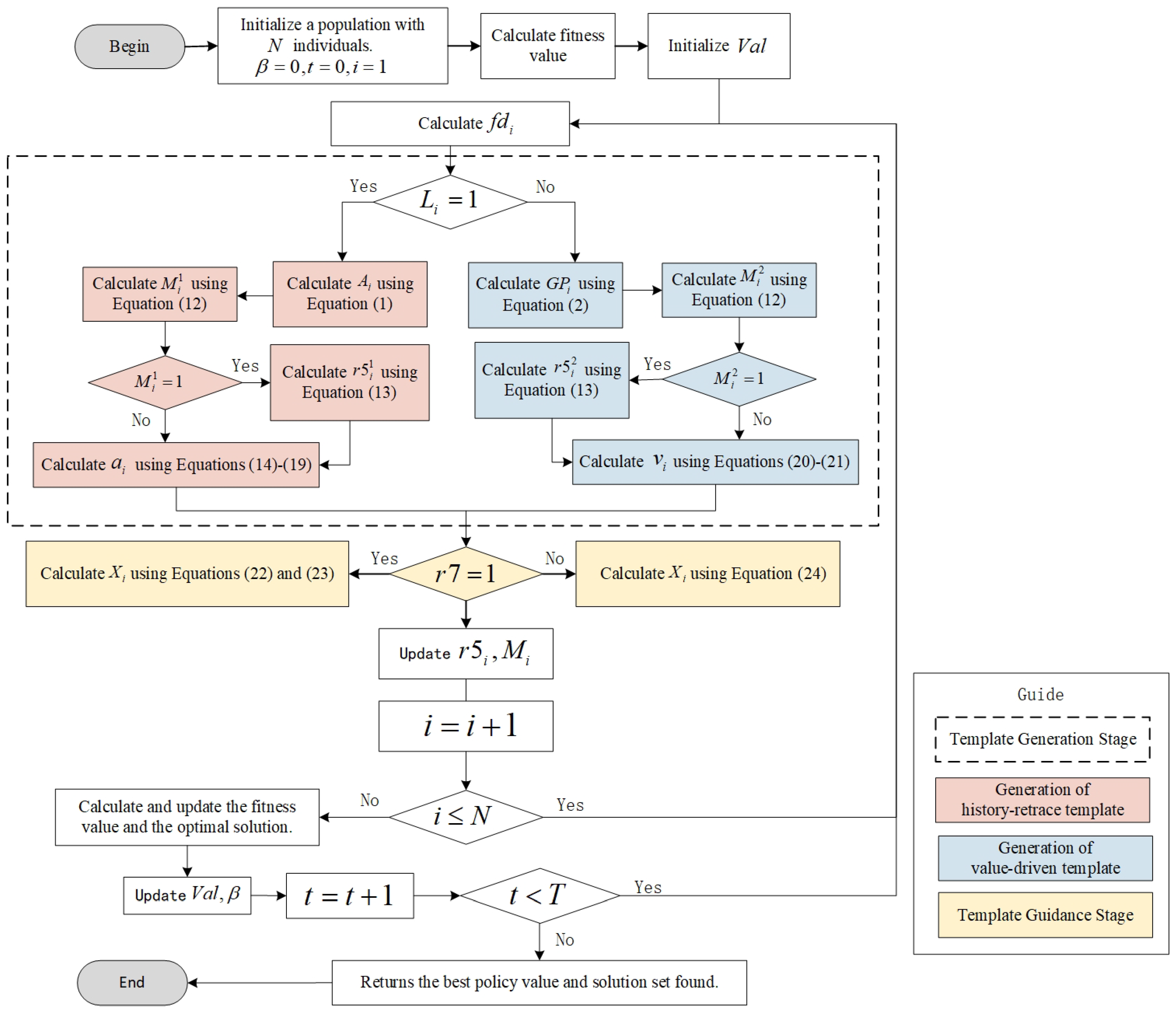
A personalized-template-guided intelligent evolutionary algorithm includes the template generation stage and the template guidance stage. The purpose of the template generation stage is to generate a guiding particle for the current particle, that is, a personalized template. Firstly, each particle randomly selects whether to generate a value-driven template or a history-retrace template to increase the diversity of exploration. Then the selection strategy of the template base point set is applied to determine the base point set of the template. Then, based on the template interval expansion strategy, the template interval surrounded by basic points is expanded. Finally, the personalized template generation strategy based on particle dimensional distribution is adopted to generate a personalized template in the corresponding interval dimension. In the template guidance stage, the template-guided knowledge transfer strategy is used to update the position of the particle. See Algorithm 1 for the specific process.

The detailed flowchart of the algorithm is shown in Figure 1. First, initialize the population and parameter values, and calculate the fitness value. Use the template interval expansion strategy to get the value $Val$, and then enter the loop. Calculate the $fd$ value of the i-th particle, and decide whether to generate the history-retrace template or the value-driven template according to the value of the random integer L. When $L_i=1$, enter the left half of the process to generate a history-retrace template, and use the selection strategy of the template base point set to calculate the base point $A_i$ of the history-retrace template by Equation (1). Then, the template generation strategy is adopted, and the $M_i$ is calculated by Equation (12), which determines whether to use the personalized template generation strategy based on particle dimensional distribution. When $M_i=1$, the dimension to be learned is obtained by Equation (13), and then the history-retrace template $a_i$ is generated by Equations (14)–(19) in combination with the interval extension value $Val$. When $M_i=2$, only the template generation strategy is used, and the history-retrace template $a_i$ is generated by Equations (14)–(19) in combination with the interval extension value $Val$. When $L_i=2$, enter the right half of the process to generate a value-driven template. Calculate the base point $G{P}_i$ of the value-driven template by Equation (2), and calculate the $M_i$ value by Equation (12). When $M_i=1$, the dimension to be learned is obtained by Equation (13), and then the value-driven template $v_i$ is generated by combining the interval spacing value with Equations (20) and (21). When $M_i=2$, $v_i$ is directly generated by combining the interval spacing value with Equations (20) and (21). After the template is generated, the algorithm enters the template guidance stage. First, a value of the random number $r7$ is calculated. When $r7=1$, a new solution $X_i$ is obtained by Equations (22) and (23), and when $r7=2$, a new solution $X_i$ is obtained by Equation (24). Update the M and $r5$ of the i-th particle. After N new solutions are generated by the above steps for N particles, the fitness value of the population is calculated, and the values of $\beta$ and $Val$ are updated. When $t\le T$, continue the above cycle. Otherwise, jump out of the loop, return to the optimal solution value and its position, and end the algorithm.

Algorithm 1: Pseudocode of PTG

Input:  popultion size N, number of iterations T Output:  the best solution of the objective function 1: $\beta \leftarrow 0$ 2: Calculate $val$ based on Equation (7) 3: Calculate the population fitness value, sort and record the optimal value 4: while $t<T$  do 5:     for $i=1$ to N do 6:         Calculate $f{d}_i$ based on Equations (8)–(11) 7:         $L_i\leftarrow Random\left(\{1,2\}\right)$ 8:         $r7\leftarrow Random\left(\right\{1,2\left\}\right)$ 9:         for $j=1$ to D do 10:            if $L_i=1$ then 11:                Calculate $A_i$ based on Equation (1) 12:                Calculate $M_i^L$ based on Equation (12) 13:                if $M_i^L=1$ then 14:                    Calculate $r{5}_i^L$ based on Equation (13) 15:                end if 16:                Generate $a_i^j$ based on Equations (14)–(19) 17:            end if 18:            if $L_i=2$ then 19:                Calculate $G{P}_i$ based on Equation (2) 20:                Calculate $M_i^L$ based on Equation (12) 21:                if $M_i^L=1$ then 22:                    Calculate $r{5}_i^L$ based on Equation (13) 23:                end if 24:                Generate $v_i^j$ based on Equations (20) and (21) 25:            end if 26:            if $r7=1$ then 27:                Generate a new particle based on Equations (22) and (23) 28:            end if 29:            if $r7=2$ then 30:                Generate a new particle based on Equation (24) 31:            end if 32:         end for 33:         Record $M_i^L$, $r{5}_i^L$ 34:     end for 35:     Calculate and rank population fitness values 36:     Update the spacing value $val$ based on Equations (3)–(7) 37:     Update $\beta$ 38: end while

2.1. Template Generation Stage

Firstly, an example is given to illustrate the brief process of template generation. Suppose there is a particle that has two dimensions. Figure 2 shows a brief process of generating a personalized template for this particle, and the same applies to the other particles. For specific details, please refer to the following content of this section. The pink part on the left of the figure represents the generation process of the history-retrace template, while the part on the right shows the generation process of the value-driven template. The length of the yellow square is the interval expansion value $Val$ obtained through the interval expansion strategy. The two small dots on the left and right of the black line segment in the figure represent the upper and lower bounds of the particle dimension value. j represents the dimension of the particle. a refers to the generated history-retrace template, and v represents the generated value-driven template.

If the particle chooses to generate a historical backtracking template, there are two possible cases for the selection of template base points. When $h<2$, there is only one template base point. When $h\ge 2$, there are two template base points. In the case of $h\ge 2$, the selection strategy of the template base point set for the history-retrace template is given. According to this strategy, two basic points are obtained in each dimension of the particle. Next, if $M=1$, the personalized template generation strategy based on particle dimensional distribution is implemented. Suppose the learning object selected by the particle is dimension 2; then, on the basis of the template base point $j=2$, the interval range is expanded with the $Val$, and the value obtained within the dashed box range is used as the value of the personalized template dimensions 1 and 2. If $M=2$, the template generation strategy is executed. Based on the base points of particle dimensions 1 and 2, add $Val$ to expand the interval range, and then generate new values within their respective ranges as the generated templates.

If the particle selects to generate a value-driven template, there is only one basis point for its template. In the template-based point selection strategy, one base point is obtained on each of the two dimensions of the particle. The following demonstrations are consistent with the historical backtracking template, but it should be noted that the specific principles and formulas of the two are different. For details, please refer to the following content of this section.

2.1.1. Selection Strategy of Template Base Point Set

The choice of base point set is very important because it determines what area the template guides the particle to explore. In particular, this algorithm stores a random particle in the merged population when the merit of each generation is unchanged, which helps the algorithm to review the previous solutions and extract historical stagnation information from them. In the specific algorithm steps, each particle randomly chooses to generate a history-retrace template or a value-driven template, which increases the diversity of exploration. In order to balance exploration and exploitation, the corresponding template base point set selection strategy is adopted under the guidance of the optimal value signal $\beta$. This strategy realizes the collaborative exploration of the population; some particles review the previous limited historical area, and some particles exploit near the optimal value.

Specifically, when the signal is the change of the previous generation’s merit, the base point of the history-retrace template is the random particles in the merged population when the merit stored in the last two generations is unchanged, while the value-driven template randomly selects one of the top three elite particles of the parent as the base point, thus realizing the collaborative exploration of the population. Some particles review the local points when they were unchanged before, and some particles are developed near the merit to jointly promote the further optimization of the solution. When the signal is the unchanged merit of the previous generation, the history-retrace template’s base point is selected from historical particles, and the value-driven template’s base point is a random particle of the parent. So as to expand the exploration scope of particles, help particles jump out of local optimization, and explore new fields.

$$A_i=\left\{\begin{array}{cc}{C}_{t1},C_{t2},\hfill & \mathrm{if}\beta =0\mathrm{and}h\ge 2\hfill \\ Q_{h-1},Q_h,\hfill & \mathrm{if}\beta =1\mathrm{and}h\ge 2\hfill \\ gbest,\hfill & \mathrm{if}\beta =1\mathrm{and}h<2\hfill \\ 1-gbest,\hfill & \mathrm{if}\beta =0\mathrm{and}h<2\hfill \end{array}\right.$$

(1)

where $A_i$ is the base point set of the history-retrace template of the i-th particle. In each iteration, randomly select one of the top N elite individuals in the merged population and store it in C. t is the current iteration number, $t=1,2,\dots ,T$, and T is the total iteration number. Where $t1$ and $t2$ are random integers of $[1,t]$. $C_{t1}$ represents the $t1$ individual in C. When the optimal value of the t-iteration population remains unchanged, a random individual of the t-iteration merged population will be stored in Q. h is the number of individuals stored in Q. N is the number of individuals in the population. $gbest$ is the location of the optimal solution of the population. $\beta$ is the optimal value signal; when the optimal value of the population changes, $\beta$ is 1, otherwise it is 0.

$$G{P}_i=\left\{\begin{array}{cc}{P}_{r4},\hfill & \mathrm{if}\beta =1\hfill \\ P_{r1},\hfill & \mathrm{if}\beta =0\hfill \end{array}\right.$$

(2)

where $G{P}_i$ is the value-driven template’s base point set of the i-th particle, P is the parent population, and $r4$ is a random integer of $[1,3]$. $r1$ is a random integer of $[1,N]$.

2.1.2. Template Interval Expansion Strategy

The selection strategy of the template base point set is only based on historical information. If the particles are guided to explore the template interval surrounded by the basic points they choose, the algorithm will easily fall into local optimization, especially in the late convergence stage. In order to solve this problem, we use Equations (3)–(7) to calculate the interval value ${Val}^j$.

When the optimal value of the population changes, the offspring population, the parent population, and the merged population all contain valid information about the distribution of optimal values. It should be noted that $V{c}^j$ is the spacing of the optimal particle population after the elite selection strategy, which lacks diversity compared with $V{\mathit{op}}^j$. Therefore, we set the parameter $\theta$ to balance the diversity and convergence of interval values. In the early stage, when the optimal value area is uncertain, the weight of $V{c}^j$ decreases gradually, while $V{\mathit{op}}^j$ increases gradually, which makes the randomness of the template interval expansion value increase gradually with iteration to help the particles jump out of the local optimization. After the midterm iteration, the weight of $V{\mathit{op}}^j$ gradually decreases, and the weight of $V{c}^j$ gradually increases, which makes the randomness of the template interval expansion value gradually decrease to help the particles gradually converge.

When the optimal value of the population is constant, the combined population may contain new distribution knowledge, because some particles in the offspring may be better than some particles in the parent. For this reason, we set the interval expansion range as the absolute difference between two random particles in the combined population to help the particle jump out of the local optimum.

$$Va{l}^j=\beta \times (V{\mathit{op}}^j\times \theta +V{c}^j\times (1-\theta ))+(1-\beta )\times Vc{r}^j$$

(3)

$$Vo{p}^j=abs({\displaystyle \frac{2}{N}}\times \sum _{i=1}^{N/2}{O}_i^j-{\displaystyle \frac{2}{N}}\times \sum _{i=1}^{N/2}{P}_i^j)$$

(4)

$$V{c}^j=abs({\displaystyle \frac{2}{N}}\times \sum _{i=1}^{N/2}C{t}_i^j-{\displaystyle \frac{2}{N}}\times \sum _{i=N/2+1}^{N}C{t}_i^j)$$

(5)

$$\theta =sin({\displaystyle \frac{t\times \pi }{T}})$$

(6)

$$Vc{r}^j=abs(C{t}_{r1}^j-C{t}_{r2}^j)$$

(7)

where $Va{l}^j$ is the interval value in the j-th dimension of the current iteration, $j=1,2,\dots ,D$, and D is the maximum dimension value. $O_i^j$ is the j-th dimension value of the i-th individual in the offspring population. $P_i^j$ is the j-th dimension value of the i-th individual of the parent population. $Vo{p}^j$ is the mean difference between the offspring population and the parent population in the j-th dimension. $Ct$ is the collection of the top N outstanding individuals in the contemporary merged population. $V{c}^j$ is the difference between the average of the top 50% of individuals and the average of the bottom 50% of individuals in $Ct$. $\theta$ is the adjustment parameter. $Vc{r}^j$ is the absolute value of the difference between random individuals in $Ct$ in the j-th dimension. $r1$ is a random integer of $[1,N]$. $r2$ is a random integer of $[1,N]$. And $r1$ is not equal to $r2$.

2.1.3. Personalized Template Generation Strategy Based on Particle Dimensional Distribution

There are three kinds of dimensional distribution of a particle: the first is concentrated distribution, the second is similar to normal distribution, and the third is random distribution. In the first two cases, just finding the mean point of the dimensional distribution can help the particle converge quickly. Therefore, we put forward the particle dimensional concentration degree to judge the particle dimensional distribution. For the particle that meets one of the first two conditions, all dimension values of the personalized template are the same, so as to guide the particle to mine near this dimension value, and then get the mean point of particle dimension distribution through the elite selection strategy.

We use the parameter $\delta$ to regulate the value of $f{d}_i$. At the initial stage of optimization, the particle dimension distribution is not stable, so $f{d}_i$ should be small. With the progress of iteration, under the elite selection strategy, the dimension distribution of particles will gradually stabilize. At this time, the personalized guidance template can be made for the particle according to its dimensional distribution to help mine their potential knowledge. At the later stage, the dimension distribution of the particle itself has been particularly stable. At this time, each dimension should be optimized and converged separately, so the value of $f{d}_i$ should be reduced.

$$f{d}_i=\left\{\begin{array}{cc}\delta ,\hfill & \mathrm{if}{w}_i=0\hfill \\ (1-{\displaystyle \frac{s_i}{w_i}})\times \delta ,\hfill & otherwise\hfill \end{array}\right.$$

(8)

$$\delta =sin\left({\displaystyle \frac{t\times \pi }{T}}\right)$$

(9)

$$s_i=abs({\displaystyle \frac{1}{D}}\times \sum _{j=1}^D{x}_i^j-{\displaystyle \frac{2}{D}}\times \sum _{j=1}^{D/2}{x}_{ir}^j)$$

(10)

$$w_i=abs(max\left(x_i\right)-min\left(x_i\right))$$

(11)

where $f{d}_i$ is the particle dimension concentration, $x_i$ is the i-th particle, $\delta$ is the concentration control parameter, and $x_{ir}$ is a new particle obtained by disrupting the dimension order in $x_i$.

When $f{d}_i$ is large, it is more likely to generate templates with the same dimension values. In addition, the dimension value the template chooses for knowledge guidance is the selection of the i-th particle of the parent in the corresponding template block with a certain probability. If the historical particle selection value is empty, it will be generated randomly. See Equations (12) and (13) below for the specific dimension value selection.

$$M{i}^L=\left\{\begin{array}{c}1, \mathrm{if}r<f{d}_i\mathrm{or}(\beta =1\mathrm{and}r<{\left(\frac{t}{T}\right)}^2\hfill \\ \hfill \mathrm{and}P{M}_i^L=1)\\ 2, \mathrm{if}r>=f{d}_i\mathrm{or}(\beta =1\mathrm{and}r<{\left(\frac{t}{T}\right)}^2\hfill \\ \hfill \mathrm{and}P{M}_i^L=2)\end{array}\right.$$

(12)

where $M{i}^L$ represents the dimension learning mode selected when the i-th particle generates the template L. If $M{i}^L=1$, a template with the same dimension value is generated. We set judgment condition 2 in our expression to be superior to condition 1. Where r is a random number between 0 and 1. $P{M}_i^L$ represents the mode of dimension learning selected when the i-th parent particle generates the template L. L is a random integer of 1 or 2. The history-retrace template is selected when $L=1$, and the value-driven template is selected when $L=2$.

$$r{5}_i^L=\left\{\begin{array}{cc}pr{5}_i^L,\hfill & \mathrm{if}\beta =1\mathrm{and}r<{\left({\displaystyle \frac{t}{T}}\right)}^2\mathrm{and}\exists pr{5}_i^L\in \mathbb{R}\hfill \\ r8,\hfill & otherwise\hfill \end{array}\right.$$

(13)

where $r{5}_i^L$ represents the dimension selected by the i-th particle when generating the L-type template. $pr{5}_i^L$ represents the dimension selected by the i-th parent particle when generating the L-type template. $r8$ is a random integer from 1 to D.

①

Generate a history-retrace template

$$a_i^j=\left\{\begin{array}{cc}f{1}_i^{r5}+(f{2}_i^{r5}-f{1}_i^{r5})\times r,\hfill & \mathrm{if}{M}_i^1=1\hfill \\ f{1}_i^j+(f{2}_i^j-f{1}_i^j)\times r,\hfill & \mathrm{if}{M}_i^1=2\hfill \end{array}\right.$$

(14)

$${f1}_i=max(min(A_i^1,A_i^2)-Val,0)$$

(15)

$$f{2}_i=min(max(A_i^1,A_i^2)+Val,1)$$

(16)

When $h\ge 2$, Equations (14)–(16) are used to generate the history-retrace template, where $a_i$ is the history-retrace template generated for the i-th particle, $f{1}_i$ is the interval lower bound, and $f{2}_i$ is the interval upper bound. $A_i^1$ represents the first value in $A_i$, and $A_i^2$ represents the second value in $A_i$.

$$a_i^j=\left\{\begin{array}{cc}e{1}_i^{r5}+(e{2}_i^{r5}-e{1}_i^{r5})\times r,\hfill & \mathrm{if}{M}_i^1=1\hfill \\ e{1}_i^j+(e{2}_i^j-e{1}_i^j)\times r,\hfill & \mathrm{if}{M}_i^1=2\hfill \end{array}\right.$$

(17)

$$e{1}_i=max((A_i-Val),0)$$

(18)

$$e{2}_i=min((A_i+Val),1)$$

(19)

When $h<2$, the history-retrace template is generated by calculating Equations (17)–(19), where $e1$ is the lower bound of the interval, and $e2$ is the upper bound of the interval.

②

Generate a value-driven template

When the optimal value changes, the change value of the particle dimension value of the optimal value of the previous generation and the current generation contains certain particle optimization trend information, and following this change rule may help the particle find the optimal value.

The particle selects the optimal value template generation method through a random number $r3$. When $r3=1$, the optimal value template generation method follows the changing law of the optimal value, and when $r3=2$, the optimal value template is generated randomly. $r9$ is used to randomly select whether the template value is increased or decreased.

Where $r3$ and $r9$ are both random integers of 1 or 2. When the random number $r3=1$, and in the corresponding selected dimension $gbes{t}^t<gbes{t}^{t-1}$, or the random number $r3=2$ and $r9=1$, the following Equation (20) is used to generate the value-driven template.

$$v_i^j=\left\{\begin{array}{cc}G{P}_i^{r5}-Va{l}^{r5}+Va{l}^{r5}\times r,\hfill & \mathrm{if}{M}_i^2=1\hfill \\ G{P}_i^j-Va{l}^j+Va{l}^j\times r,\hfill & \mathrm{if}{M}_i^2=2\hfill \end{array}\right.$$

(20)

When $r3=1$ and $gbes{t}^t\ge gbes{t}^{t-1}$ or $r3=2$ and $r9=2$, the following Equation (21) is used to generate the value-driven template.

$$v_i^j=\left\{\begin{array}{cc}G{P}_i^{r5}+Va{l}^{r5}\times r,\hfill & \mathrm{if}{M}_i^2=1\hfill \\ G{P}_i^j+Va{l}^j\times r,\hfill & \mathrm{if}{M}_i^2=2\hfill \end{array}\right.$$

(21)

where $v_i^j$ is the value-driven template generated for the i-th individual in the j-th dimension.

2.2. Template Guidance Stage

Particle optimization needs to explore the right spatial range at the right time node. After the template generation stage, we obtained the space that needs to be explored emphatically. Therefore, in the template guidance stage, we adopt the template-guided knowledge transfer strategy. The strategy, aimed at improving the optimization efficiency of particles, further controls the step size of particles based on the current iteration’s time node, guiding them to search for key optimal points within the focused exploration space. $r7$ is a random integer of 1 or 2. In order to increase randomness, the particle uses $r7$ to randomly select particle-led knowledge transfer or template-led knowledge transfer. When $r<f{d}_i$, all dimensions use the same random number. In order to balance the ability to optimize exploration and development, it is not necessary to constrain step size and direction through time when the optimal value changes.

$$rd1={\displaystyle \frac{t}{T}}+((2-{\displaystyle \frac{t}{2\times T}})-{\displaystyle \frac{t}{T}})\times r$$

(22)

$$\begin{array}{c}{X}_i=m_i+(m_i-x_i)\times sin(rd1\times \pi )\times (1-\beta )\times (t/T)+\\ \beta \times sin(r\times 2\times \pi )\times (m_i-x_i)\end{array}$$

(23)

When $r7=1$, the above Equations (22) and (23) generate new particles $X_i$ through knowledge transfer. $rd1$ is the regulatory parameter, and $m_i$ is the template selected by the i-th individual. When $L=1$, $m_i=a_i$, and when $L=2$, $m_i=v_i$.

When the figure of merit is constant, the knowledge transfer strategy with the template as the main learning object will gradually move closer to the particle direction with iteration, and the step size will gradually increase.

$$\begin{array}{c}{X}_i=x_i+(x_i-m_i)\times (cos(2\times \pi \times r6)\times (1-\beta )\times \\ (1-{\displaystyle \frac{t}{T}})+\beta \times sin(r\times 2\times \pi )\times (x_i-m_i)\end{array}$$

(24)

When $r7=2$, Equation (24) generates new particles $X_i$ through knowledge transfer. $r6$ is a random number in the range $[-1,1]$.

When the figure of merit is constant, the direction of the knowledge transfer strategy with the particle itself as the core is random, and with the iteration, the step size of the particle to the template gradually decreases.

2.3. Computation Complexity

This section analyzes the time complexity and algorithm running time of PTG. Suppose the population size is N, the number of iterations is T, and the problem dimension is D. The main loop of the algorithm executes T iterations, and in each iteration, the algorithm needs to generate particles through the template generation stage and the template guidance stage. In the template generation stage, the dimension analysis value $fd$ of each particle needs to be calculated, so the time complexity is $O(N\ast D\ast T)$. In the template interval expansion strategy, the $Val$ value of each particle is the same in the current iteration, so the computational complexity is $O(N/2\ast D\ast T)$. The time complexity of generating history-retrace templates or value-driven templates for particles is $O(N\ast D\ast T)$. In the template guidance stage, the time complexity of both boot modes is $O(N\ast D\ast T)$. Therefore, the overall time complexity of the algorithm is $O(N\ast D\ast T)+O(N/2\ast D\ast T)+O(N\ast D\ast T)+O(N\ast D\ast T)$. Since the constant term can be ignored, it can be reduced to $O(N\ast D\ast T)$.

3. Results

3.1. Experimental Setup

(1)

Benchmark function: CEC2005 [46] data set containing 23 benchmark test functions is adopted. Where F1–F13 are high-dimensional problems. The functions of F1–F5 are unimodal. F6 function is a step function, F7 function is a noisy quartic function, and F8–F13 is a multimodal function. F14–F23 are low-dimensional functions with only a few local minima. CEC2022 [47] test function with complex OP ability is also used to evaluate the performance of the algorithm and verify the algorithm. In CEC2022, the function consists of 12 benchmark functions, including unimodal, multimodal, mixed, and compound functions, where F1 is unimodal, F2–F5 are multimodal, F6–F8 are mixed, which can be unimodal or multimodal, and F9–F12 are compound and multimodal.

(2)

Comparison algorithm: We compare the proposed algorithm with the classical algorithm, which are Moth-Flame Optimization algorithm (MFO) [35], Whale Optimization Algorithm (WOA) [36], Harris Hawks optimization algorithm (HHO) [37], and Tunicate Swarm Algorithm (TSA) [39]. We also compare the proposed algorithm with the latest and most advanced optimization algorithm, which are Educational Competitive Optimization (ECO) [26] (Q2, 2024), Coati Optimization Algorithm (COA) [38] (Q1, 2023), Reptile Search Algorithm (RSA) [40] (Q1, 2022), Fata Morgana Algorithm (FATA) [48] (Q2, 2024), and Hippopotamus Optimization algorithm (HO) [49] (Q2, 2024). See

Table 1. Algorithm parameters and their values.

Algorithm	Parameter	Value
FATA	$\alpha$	0.2
ECO	H	0.5
	a	4
HO	-	-
COA	-	-
RSA	a	0.1
	$\beta$	0.005
TSA	$P_{min}$	1
	$P_{max}$	4
HHO	$E_0$	[−1, 1)
WOA	Convergence parameter (a)	Linear reduction 2 to 0
MFO	b	1
	r	Linear reduction −1 to −2

for the detailed settings of control parameters, in which the population size of all algorithms is set to 30, the number of iterations is 1000, and the maximum number of evaluations is 30,000.

(3)

experimental environment: All experiments were carried out under the 64-bit version of Windows 11 operating system with MATLAB R2022a software, using Intel Core, with a basic frequency of 1.00 GHz and a maximum turbo frequency of 1.2 GHz, and a processor with 8 logic cores.

3.2. Ablation Experiment

To verify the validity of our proposed framework, we set up the ablation study. The specific results are shown in

Table 2. Ablation experiment of PTG on CEC2022.

Functions	Metric	PTG	PTG-noQ	PTG-noPDD	PTG-noIE
F1	mean	8.17 × 103	9.44 × 103	1.95 × 104	8.32 × 103
	std	2.70 × 103	3.79 × 103	3.51 × 103	3.70 × 103
F2	mean	4.52 × 102	4.60 × 102	4.63 × 102	4.70 × 102
	std	1.49 × 101	2.14 × 101	6.27	2.81 × 101
F3	mean	6.00 × 102	6.01 × 102	6.07 × 102	6.16 × 102
	std	3.12 × 10−1	3.30 × 10−1	1.20	8.35
F4	mean	8.26 × 102	8.28 × 102	8.52 × 102	8.64 × 102
	std	9.37	1.07 × 101	1.29 × 101	1.81 × 101
F5	mean	9.15 × 102	9.19 × 102	9.30 × 102	1.68 × 103
	std	1.58 × 101	2.42 × 101	1.35 × 101	6.06 × 102
F6	mean	6.93 × 103	9.42 × 103	4.12 × 105	7.20 × 103
	std	5.72 × 103	6.50 × 103	2.12 × 105	6.66 × 103
F7	mean	2.04 × 103	2.05 × 103	2.07 × 103	2.10 × 103
	std	1.22 × 101	1.37 × 101	1.38 × 101	4.16 × 101
F8	mean	2.226 × 103	2.227 × 103	2.231 × 103	2.233 × 103
	std	2.61	2.44	1.92	2.22 × 101
F9	mean	2.48 × 103	2.48 × 103	2.50 × 103	2.48 × 103
	std	3.86 × 10−2	9.00 × 10−2	6.36	1.80 × 10−1
F10	mean	2.56 × 103	2.61 × 103	2.50 × 103	3.15 × 103
	std	1.98 × 102	3.66 × 102	1.90 × 10−1	5.55 × 102
F11	mean	2.92 × 103	2.94 × 103	3.19 × 103	2.97 × 103
	std	1.19 × 102	1.05 × 102	6.78 × 101	1.75 × 102
F12	mean	2.95 × 103	2.95 × 103	2.96 × 103	2.97 × 103
	std	6.74	9.64	7.78	1.92 × 101

.

(1)

PTG-noQ means that the history-retrace template’s base point set does not extract the stagnant historical value Q in Equation (1). It can be seen from the table that the stability and accuracy of the PTG solution are better than those of PTG-noQ, which shows that the timely backtracking and mining of historical stagnation optimal values can help the algorithm refine the search solution and reduce time-consuming shocks and wrong searches.

(2)

PTG-noPDD refers to adopting the template generation strategy that is not based on the particle’s dimension distribution, specifically, $M=2$. PTG is superior to PTG-noPDD in all 11 functions, especially F1, F6, and F11, which indicates that the dimensional distribution information of the particle itself is very important for solving unimodal function problems, mixed function problems, and complex and multimodal function problems. It also shows that the personalized template generation strategy based on particle dimensional distribution can adjust the dimension value of the template promptly according to the dimensional distribution law of the particle itself and guide the particle to efficiently search for optimization.

(3)

PTG-noIE stands for eliminating the template interval expansion strategy. PTG is superior to PTG-noIE in 12 functions, especially in complex functions such as F5, F6, and F10. This shows that the template interval expansion strategy can help particles jump out of local optimization and enhance the exploration ability of the algorithm.

It can also be seen from the ablation experiment that the function value rarely changes in order of magnitude after removing the key strategy, which shows the effectiveness of the algorithm framework guided by the figure of merit signal.

3.3. Comparison of PTG with Other Algorithms

3.3.1. Analysis of Experimental Results of CEC2005 Test Function

The comparison results between the algorithm and the comparison algorithm based on the CEC2005 test set are shown in

Table 3. Performance metrics for algorithms (PTG, WOA, HHO, COA, TSA) on CEC2005 (F1–F23).

Functions	Metric	PTG	WOA	HHO	COA	TSA
F1	mean	0	$4.23\times {10}^{-149}$	$1.90\times {10}^{-184}$	0	$3.61\times {10}^{-46}$
	std	0	$2.29\times {10}^{-148}$	0	0	$1.62\times {10}^{-45}$
	rank	1	7	6	1	9
F2	mean	0	$9.94\times {10}^{-108}$	$1.28\times {10}^{-94}$	0	$2.71\times {10}^{-49}$
	std	0	$3.01\times {10}^{-107}$	$6.99\times {10}^{-94}$	0	$5.92\times {10}^{-49}$
	rank	1	6	7	1	9
F3	mean	0	$1.901\times {10}^1$	$3.22\times {10}^{-156}$	0	$5.78\times {10}^{-54}$
	std	0	$3.278\times {10}^1$	$1.76\times {10}^{-155}$	0	$1.74\times {10}^{-53}$
	rank	1	10	6	1	8
F4	mean	0	$8.70\times {10}^{-1}$	$1.80\times {10}^{-91}$	0	$1.55\times {10}^{-21}$
	std	0	$2.59$	$8.77\times {10}^{-91}$	0	$4.58\times {10}^{-21}$
	rank	1	10	6	1	8
F5	mean	$1.15\times {10}^{-26}$	$6.19$	$7.35\times {10}^{-4}$	0	$8.49$
	std	0	$4.10\times {10}^{-1}$	$9.41\times {10}^{-4}$	0	$9.20\times {10}^{-1}$
	rank	2	8	3	1	9
F6	mean	0	$6.35\times {10}^{-5}$	$1.32\times {10}^{-5}$	0	$1.12$
	std	0	$6.57\times {10}^{-5}$	$1.86\times {10}^{-5}$	0	$4.00\times {10}^{-1}$
	rank	1	7	5	1	9
F7	mean	$1.01\times {10}^{-4}$	$1.10\times {10}^{-3}$	$1.10\times {10}^{-4}$	$2.60\times {10}^{-5}$	$1.60\times {10}^{-3}$
	std	$6.68\times {10}^{-5}$	$1.10\times {10}^{-3}$	$1.12\times {10}^{-4}$	$2.40\times {10}^{-5}$	$6.93\times {10}^{-4}$
	rank	5	8	6	1	9
F8	mean	$-4.19\times {10}^3$	$-3.66\times {10}^3$	$-4.18\times {10}^3$	$-4.19\times {10}^3$	$-2.52\times {10}^3$
	std	$2.78\times {10}^{-12}$	$6.6747\times {10}^2$	$7.9308\times {10}^1$	$2.80\times {10}^{-3}$	$3.5426\times {10}^2$
	rank	1	7	5	3	9
F9	mean	0	$4.74\times {10}^{-16}$	0	0	$2.56364\times {10}^1$
	std	0	$2.59\times {10}^{-15}$	0	0	$1.225\times {10}^1$
	rank	1	8	1	1	10
F10	mean	$4.44\times {10}^{-16}$	$3.05\times {10}^{-15}$	$4.44\times {10}^{-16}$	$4.44\times {10}^{-16}$	$1.13$
	std	0	$2.46\times {10}^{-15}$	0	0	$1.63$
	rank	1	8	1	1	10
F11	mean	0	$2.40\times {10}^{-2}$	0	0	$4.39\times {10}^{-1}$
	std	0	$6.12\times {10}^{-2}$	0	0	$2.55\times {10}^{-1}$
	rank	1	8	1	1	10
F12	mean	$4.71\times {10}^{-32}$	$2.90\times {10}^{-3}$	$5.50\times {10}^{-6}$	$4.71\times {10}^{-32}$	$2.56$
	std	$1.67\times {10}^{-47}$	$5.40\times {10}^{-3}$	$6.74\times {10}^{-6}$	$1.67\times {10}^{-47}$	$3.71$
	rank	1	6	4	1	10
F13	mean	$1.35\times {10}^{-32}$	$7.90\times {10}^{-3}$	$2.96\times {10}^{-5}$	$1.35\times {10}^{-32}$	$6.38\times {10}^{-1}$
	std	$5.57\times {10}^{-48}$	$1.84\times {10}^{-2}$	$5.35\times {10}^{-5}$	$5.57\times {10}^{-48}$	$2.70\times {10}^{-1}$
	rank	1	7	4	1	10
F14	mean	$9.98\times {10}^{-1}$	$2.1781$	$1.0311$	$9.98\times {10}^{-1}$	$1.05407\times {10}^1$
	std	0	$2.49$	$1.82\times {10}^{-1}$	$9.73\times {10}^{-11}$	$3.98$
	rank	1	6	4	3	10
F15	mean	$3.38\times {10}^{-4}$	$5.98\times {10}^{-4}$	$3.63\times {10}^{-4}$	$4.23\times {10}^{-4}$	$1.31\times {10}^{-2}$
	std	$1.67\times {10}^{-4}$	$3.24\times {10}^{-4}$	$1.66\times {10}^{-4}$	$2.40\times {10}^{-4}$	$2.00\times {10}^{-2}$
	rank	3	6	4	5	10
F16	mean	$-1.0316$	$-1.0316$	$-1.0316$	$-1.0316$	$-1.0264$
	std	$6.78\times {10}^{-16}$	$1.31\times {10}^{-10}$	$9.31\times {10}^{-12}$	$4.41\times {10}^{-5}$	$1.20\times {10}^{-2}$
	rank	1	5	4	8	10
F17	mean	$3.979\times {10}^{-1}$	$3.979\times {10}^{-1}$	$3.979\times {10}^{-1}$	$3.984\times {10}^{-1}$	$3.979\times {10}^{-1}$
	std	0	$4.33\times {10}^{-7}$	$1.14\times {10}^{-7}$	$1.50\times {10}^{-3}$	$2.04\times {10}^{-5}$
	rank	1	6	5	9	8
F18	mean	$3.00$	$3.00$	$3.00$	$3.38$	$6.60$
	std	$1.36\times {10}^{-15}$	$2.57\times {10}^{-5}$	$4.78\times {10}^{-8}$	$8.87\times {10}^{-1}$	$9.34$
	rank	1	7	5	8	9
F19	mean	$-3.8628$	$-3.8585$	$-3.861$	$-3.8206$	$-3.8624$
	std	$2.71\times {10}^{-15}$	$5.50\times {10}^{-3}$	$2.20\times {10}^{-3}$	$4.66\times {10}^{-2}$	$1.40\times {10}^{-3}$
	rank	1	7	6	10	4
F20	mean	$-3.2744$	$-3.2325$	$-3.1903$	$-2.7113$	$-3.2051$
	std	$5.92\times {10}^{-2}$	$1.16\times {10}^{-1}$	$9.15\times {10}^{-2}$	$3.25\times {10}^{-1}$	$1.91\times {10}^{-1}$
	rank	2	4	8	9	7
F21	mean	$-9.9848$	$-9.3022$	$-5.2232$	$-10.1532$	$-6.0689$
	std	$9.22\times {10}^{-1}$	$1.93$	$9.23\times {10}^{-1}$	$7.30\times {10}^{-5}$	$2.94$
	rank	4	6	9	2	8
F22	mean	$-10.4029$	$-8.7292$	$-5.4334$	$-10.4028$	$-7.8476$
	std	$8.73\times {10}^{-16}$	$2.63$	$1.32$	$2.17\times {10}^{-5}$	$3.23$
	rank	1	6	9	3	7
F23	mean	$-10.5364$	$-8.629$	$-5.1279$	$-10.5363$	$-7.337$
	std	$2.06\times {10}^{-15}$	$3.05$	$6.64\times {10}^{-4}$	$3.16\times {10}^{-5}$	$3.58$
	rank	1	6	10	3	8

and

Table 4. Performance metrics for algorithms (RSA, FATA, MFO, ECO, HO) on CEC2005 (F1–F23).

Functions	Metric	RSA	FATA	MFO	ECO	HO
F1	mean	0	0	$2.00\times {10}^3$	$6.72\times {10}^{-111}$	0
	std	0	0	$4.07\times {10}^3$	$3.48\times {10}^{-110}$	0
	rank	1	1	10	8	1
F2	mean	0	0	1	$2.73\times {10}^{-59}$	0
	std	0	0	$3.05$	$1.50\times {10}^{-58}$	0
	rank	1	1	10	8	1
F3	mean	0	0	$1.94\times {10}^{-6}$	$3.10\times {10}^{-99}$	0
	std	0	0	$6.77\times {10}^{-6}$	$1.70\times {10}^{-98}$	0
	rank	1	1	9	7	1
F4	mean	0	0	$4.15\times {10}^{-1}$	$5.92\times {10}^{-57}$	0
	std	0	0	$5.76\times {10}^{-1}$	$3.24\times {10}^{-56}$	0
	rank	1	1	9	7	1
F5	mean	$2.921\times {10}^{-1}$	$2.8708$	$3.22\times {10}^3$	$5.6281$	$9.92\times {10}^{-4}$
	std	$1.60$	$3.25$	$1.64\times {10}^4$	$4.51\times {10}^{-1}$	$8.10\times {10}^{-4}$
	rank	5	6	10	7	4
F6	mean	$1.9942$	$4.39\times {10}^{-2}$	$4.82\times {10}^{-30}$	$3.90\times {10}^{-14}$	$2.15\times {10}^{-5}$
	std	$3.26\times {10}^{-1}$	$6.8\times {10}^{-2}$	$1.50\times {10}^{-29}$	$7.68\times {10}^{-14}$	$1.29\times {10}^{-5}$
	rank	10	8	3	4	6
F7	mean	$5.02\times {10}^{-5}$	$3.35\times {10}^{-5}$	$7.2\times {10}^{-3}$	$1.36\times {10}^{-4}$	$8.42\times {10}^{-5}$
	std	$4.11\times {10}^{-5}$	$3.27\times {10}^{-5}$	$5.2\times {10}^{-3}$	$1.09\times {10}^{-4}$	$6.42\times {10}^{-5}$
	rank	3	2	10	7	4
F8	mean	$-1.96\times {10}^3$	$-4.19\times {10}^3$	$-3.16\times {10}^3$	$-3.93\times {10}^3$	$-4.19\times {10}^3$
	std	$6.232\times {10}^1$	$1.23\times {10}^{-2}$	$3.46\times {10}^2$	$3.08\times {10}^2$	$4.38\times {10}^{-4}$
	rank	10	4	8	6	2
F9	mean	0	0	$2.2062\times {10}^1$	0	0
	std	0	0	$1.26044\times {10}^1$	0	0
	rank	1	1	9	1	1
F10	mean	$4.44\times {10}^{-16}$	$4.44\times {10}^{-16}$	$6.408\times {10}^{-1}$	$4.44\times {10}^{-16}$	$4.44\times {10}^{-16}$
	std	0	0	$3.30$	0	0
	rank	1	1	9	1	1
F11	mean	0	0	$1.49\times {10}^{-1}$	0	0
	std	0	0	$8.8\times {10}^{-2}$	0	0
	rank	1	1	9	1	1
F12	mean	$7.75\times {10}^{-1}$	$3.9\times {10}^{-3}$	$5.79\times {10}^{-1}$	$2.03\times {10}^{-14}$	$2.28\times {10}^{-5}$
	std	$5.00\times {10}^{-1}$	$1.02\times {10}^{-2}$	$1.32$	$6.43\times {10}^{-14}$	$2.08\times {10}^{-5}$
	rank	9	7	8	3	5
F13	mean	$2.06\times {10}^{-31}$	$1.30\times {10}^{-2}$	$7.70\times {10}^{-3}$	$3.48\times {10}^{-2}$	$1.35\times {10}^{-4}$
	std	$2.23\times {10}^{-31}$	$3.16\times {10}^{-2}$	$1.45\times {10}^{-2}$	$1.80\times {10}^{-1}$	$1.51\times {10}^{-4}$
	rank	3	8	6	9	5
F14	mean	$4.2171$	$3.3325$	$3.1292$	$1.1629$	$9.98\times {10}^{-1}$
	std	$3.36$	$4.7488$	$2.9899$	$7.38\times {10}^{-1}$	$2.43\times {10}^{-14}$
	rank	9	8	7	5	2
F15	mean	$1.40\times {10}^{-3}$	$3.15\times {10}^{-4}$	$1.20\times {10}^{-3}$	$3.20\times {10}^{-3}$	$3.07\times {10}^{-4}$
	std	$3.96\times {10}^{-4}$	$3.03\times {10}^{-5}$	$1.40\times {10}^{-3}$	$6.90\times {10}^{-3}$	$3.45\times {10}^{-9}$
	rank	8	2	7	9	1
F16	mean	$-1.0307$	$-1.0316$	$-1.0316$	$-1.0316$	$-1.0316$
	std	$1.60\times {10}^{-3}$	$3.84\times {10}^{-8}$	$6.78\times {10}^{-16}$	$2.88\times {10}^{-9}$	$1.62\times {10}^{-12}$
	rank	9	7	1	6	3
F17	mean	$4.072\times {10}^{-1}$	$3.979\times {10}^{-1}$	$3.979\times {10}^{-1}$	$3.979\times {10}^{-1}$	$3.979\times {10}^{-1}$
	std	$1.13\times {10}^{-2}$	$1.56\times {10}^{-6}$	0	$1.32\times {10}^{-9}$	$2.19\times {10}^{-10}$
	rank	10	7	1	4	3
F18	mean	$6.62$	3	3	3	3
	std	$9.40$	$3.93\times {10}^{-7}$	$1.84\times {10}^{-15}$	$1.91\times {10}^{-15}$	$3.47\times {10}^{-11}$
	rank	10	6	2	3	4
F19	mean	$-3.8358$	$-3.8623$	$-3.8628$	$-3.837$	$-3.8628$
	std	$2.10\times {10}^{-2}$	$5.92\times {10}^{-4}$	$2.71\times {10}^{-15}$	$1.41\times {10}^{-1}$	$1.94\times {10}^{-9}$
	rank	9	5	1	8	3
F20	mean	$-2.6615$	$-3.2145$	$-3.2319$	$-3.2586$	$-3.2850$
	std	$4.46\times {10}^{-1}$	$5.99\times {10}^{-2}$	$6.32\times {10}^{-2}$	$6.03\times {10}^{-2}$	$5.75\times {10}^{-2}$
	rank	10	6	5	3	1
F21	mean	$-5.0552$	$-10.1531$	$-6.3007$	$-9.9024$	$-10.1532$
	std	$3.84\times {10}^{-7}$	$1.46\times {10}^{-4}$	$3.34$	$1.37$	$1.15\times {10}^{-7}$
	rank	10	3	7	5	1
F22	mean	$-5.0877$	$-10.4027$	$-7.7248$	$-9.5259$	$-10.4029$
	std	$1.02\times {10}^{-6}$	$1.82\times {10}^{-4}$	$3.4044$	$2.6962$	$1.77\times {10}^{-7}$
	rank	10	4	8	5	2
F23	mean	$-5.1285$	$-10.5362$	$-7.6631$	$-9.0018$	$-10.5364$
	std	$1.61\times {10}^{-6}$	$1.61\times {10}^{-4}$	$3.62$	$3.14$	$9.97\times {10}^{-8}$
	rank	9	4	7	5	2

. In the table, we take the average of the optimal solutions obtained by the algorithm in 30 independent runs as the mean of the algorithm. Calculate the standard deviation of these 30 solutions to measure the average deviation degree of data points from the mean. The larger the value, the more dispersed the data distribution. The 10 algorithms are ranked based on their standard deviations and means. The smaller the ranking value, the better the algorithm’s performance. The convergence of the algorithm is shown in Figure 3, where the vertical axis represents the mean value of the algorithm at the same iteration time point during 30 independent runs. For example, the vertical axis corresponding to the point of iteration 1 on the horizontal axis is the mean value of the 30 points with an iteration time of 1 during the 30 independent runs. Because the algorithm converges quickly on some functions, in order to show the convergence trend of the graph more obviously, in the functions F1, F2, F5, F6, F7, F11, F12, F13, F14, F15, F16, F17, and F18, only the first 50 of the 1000 mean points of the algorithm and the solution values corresponding to the 200th, 400th, 600th, 800th, and 1000th iterations are taken as the x-coordinate points.

As can be seen from Table 3 and Table 4. In the comparison of unimodal benchmark functions, PTG ranks first among F1-F4 and F6 functions, and the final result of the F5 function is far superior to other algorithms except COA, with a standard deviation of 0 and ranking second. It can be seen from Figure 3 that the convergence speed of the PTG algorithm is not always the fastest among the F1–F4 and F6 functions, but it converges to a solution better than or equal to that of other algorithms before about 50 iterations. In the F4 function, although its convergence speed is slower than that of the four algorithms, it is better than their function values, so PTG has the ability to maintain diversity when converging. As can be seen from Figure 4, in F1–F7, the data of PTG running independently for 30 times presents a centralized distribution, and compared with other algorithms, there are no outliers. A “+” in the figure indicates an outlier of the data. To sum up, it can be seen that the algorithm is effective in solving the unimodal benchmark function problem.

The performance analysis of the algorithm in the F8-F13 multi-dimensional and multimodal test function of CEC2005 is as follows. As can be seen from Table 3 and Table 4, the PTG algorithm always ranks first, and the standard deviation is always the minimum. As can be seen from Figure 3, the PTG algorithm can always converge to a solution better than or equal to other algorithms 200 generations ago. As can be seen from Figure 4, the data of the PTG algorithm is the most concentrated, and there are no outliers. In summary, it can be seen that the algorithm has excellent global search ability.

The evaluation of this algorithm in the multimodal benchmark function of F14–F23 is as follows. As can be seen from Table 3 and Table 4, except for the functions of F15, F20, and F21, the algorithm ranks first in the other seven functions and second only to the HO algorithm in the function of F20. From Figure 3, in the F22 function, the algorithm found the excellent solution again after converging to the excellent value and maintaining a certain number of iterations, indicating that the algorithm has a strong ability to balance exploration and exploitation.

3.3.2. Analysis of Experimental Results of CEC2022 Test Function

The comparison results of PTG and other algorithms on CEC2022 are shown in

Table 5. Performance Comparison of Algorithms (PTG, WOA, HHO, COA, TSA) on CEC2022.

Function	Metric	PTG	WOA	HHO	COA	TSA
F1	mean	$8.32\times {10}^3$	$2.43\times {10}^4$	$8.79\times {10}^3$	$4.56\times {10}^4$	$1.75\times {10}^4$
	std	$3.16\times {10}^3$	$6.46\times {10}^3$	$3.41\times {10}^3$	$1.22\times {10}^4$	$6.45\times {10}^3$
	rank	1	7	2	10	6
	time	$3.50$	$8.42\times {10}^{-2}$	$2.45\times {10}^{-1}$	$1.87\times {10}^{-1}$	$1.34\times {10}^{-1}$
F2	mean	$4.52\times {10}^2$	$5.66\times {10}^2$	$4.94\times {10}^2$	$3.09\times {10}^3$	$7.74\times {10}^2$
	std	$1.49\times {10}^1$	$6.11\times {10}^1$	$3.87\times {10}^1$	$8.97\times {10}^2$	$2.06\times {10}^2$
	rank	1	7	4	10	8
	time	$3.63$	$8.45\times {10}^{-2}$	$2.41\times {10}^{-1}$	$1.59\times {10}^{-1}$	$1.45\times {10}^{-1}$
F3	mean	$6.00\times {10}^2$	$6.68\times {10}^2$	$6.60\times {10}^2$	$6.8079\times {10}^2$	$6.62\times {10}^2$
	std	$3.12\times {10}^{-1}$	$1.17\times {10}^1$	$7.05$	$1.07\times {10}^1$	$1.44\times {10}^1$
	rank	1	8	6	9	7
	time	$3.58$	$1.85\times {10}^{-1}$	$5.15\times {10}^{-1}$	$4.18\times {10}^{-1}$	$2.34\times {10}^{-1}$
F4	mean	$8.28\times {10}^2$	$9.2405\times {10}^2$	$8.9052\times {10}^2$	$9.7333\times {10}^2$	$9.5783\times {10}^2$
	std	$1.04\times {10}^1$	$3.00\times {10}^1$	$1.33\times {10}^1$	$1.75\times {10}^1$	$3.12\times {10}^1$
	rank	1	7	4	10	8
	time	$3.55$	$1.24\times {10}^{-1}$	$3.14\times {10}^{-1}$	$2.37\times {10}^{-1}$	$1.63\times {10}^{-1}$
F5	mean	$9.15\times {10}^2$	$3.99\times {10}^3$	$2.87\times {10}^3$	$3.50\times {10}^3$	$4.16\times {10}^3$
	std	$1.57559\times {10}^1$	$1.36\times {10}^3$	$2.5840\times {10}^2$	$3.9193\times {10}^2$	$1.52\times {10}^3$
	rank	1	9	5	8	10
	time	$3.48$	$1.24\times {10}^{-1}$	$3.34\times {10}^{-1}$	$2.43\times {10}^{-1}$	$1.66\times {10}^{-1}$
F6	mean	$6.93\times {10}^3$	$7.62\times {10}^5$	$1.07\times {10}^5$	$2.22\times {10}^9$	$1.65\times {10}^8$
	std	$5.72\times {10}^3$	$1.14\times {10}^6$	$6.18\times {10}^4$	$1.07\times {10}^9$	$4.61\times {10}^8$
	rank	1	6	4	10	8
	time	$3.54$	$9.58\times {10}^{-2}$	$2.70\times {10}^{-1}$	$2.02\times {10}^{-1}$	$1.55\times {10}^{-1}$
F7	mean	$2.04\times {10}^3$	$2.21\times {10}^3$	$2.19\times {10}^3$	$2.22\times {10}^3$	$2.25\times {10}^3$
	std	$1.22\times {10}^1$	$8.44\times {10}^1$	$6.68\times {10}^1$	$4.82\times {10}^1$	$9.53\times {10}^1$
	rank	1	7	6	8	10
	time	$3.97$	$2.30\times {10}^{-1}$	$6.05\times {10}^{-1}$	$5.57\times {10}^{-1}$	$2.78\times {10}^{-1}$
F8	mean	$2.23\times {10}^3$	$2.27\times {10}^3$	$2.28\times {10}^3$	$2.43\times {10}^3$	$2.41\times {10}^3$
	std	$2.61$	$4.86\times {10}^1$	$7.74\times {10}^1$	$1.36\times {10}^2$	$3.84\times {10}^2$
	rank	1	4	7	9	8
	time	$3.96$	$2.74\times {10}^{-1}$	$6.82\times {10}^{-1}$	$6.42\times {10}^{-1}$	$3.23\times {10}^{-1}$
F9	mean	$2.48\times {10}^3$	$2.57\times {10}^3$	$2.51\times {10}^3$	$3.48\times {10}^3$	$2.71\times {10}^3$
	std	$3.86\times {10}^{-2}$	$4.82\times {10}^1$	$3.69\times {10}^1$	$3.51\times {10}^2$	$1.62\times {10}^2$
	rank	1	7	4	10	8
	time	$3.75$	$2.22\times {10}^{-1}$	$5.64\times {10}^{-1}$	$5.37\times {10}^{-1}$	$2.70\times {10}^{-1}$
F10	mean	$2.68\times {10}^3$	$4.69\times {10}^3$	$3.76\times {10}^3$	$6.24\times {10}^3$	$5.03\times {10}^3$
	std	$5.45\times {10}^2$	$1.09\times {10}^3$	$7.84\times {10}^2$	$1.45\times {10}^3$	$1.24\times {10}^3$
	rank	1	7	5	10	9
	time	$3.70$	$1.91\times {10}^{-1}$	$5.20\times {10}^{-1}$	$4.07\times {10}^{-1}$	$2.30\times {10}^{-1}$
F11	mean	$2.92\times {10}^3$	$3.66\times {10}^3$	$3.10\times {10}^3$	$9.07\times {10}^3$	$6.83\times {10}^3$
	std	$1.19\times {10}^2$	$7.79\times {10}^2$	$2.01\times {10}^2$	$5.60\times {10}^2$	$1.11\times {10}^3$
	rank	1	5	4	9	7
	time	$3.93$	$3.12\times {10}^{-1}$	$6.82\times {10}^{-1}$	$6.44\times {10}^{-1}$	$3.67\times {10}^{-1}$
F12	mean	$2.9471\times {10}^3$	$3.1041\times {10}^3$	$3.1355\times {10}^3$	$3.6458\times {10}^3$	$3.3283\times {10}^3$
	std	$6.74\times {10}^1$	$1.21\times {10}^2$	$1.25\times {10}^2$	$3.09\times {10}^2$	$1.87\times {10}^2$
	rank	1	4	7	10	9
	time	$3.86$	$3.27\times {10}^{-1}$	$7.76\times {10}^{-1}$	$7.27\times {10}^{-1}$	$3.70\times {10}^{-1}$

and

Table 6. Performance Comparison of Algorithms (RSA, FATA, MFO, ECO, HO) on CEC2022.

Function	Metric	RSA	FATA	MFO	ECO	HO
F1	mean	$3.30\times {10}^4$	$1.11\times {10}^4$	$3.88\times {10}^4$	$1.10\times {10}^4$	$1.41\times {10}^4$
	std	$9.03\times {10}^3$	$4.71\times {10}^3$	$2.08\times {10}^4$	$6.95\times {10}^3$	$7.06\times {10}^3$
	rank	8	4	9	3	5
	time	$8.05\times {10}^{-1}$	$1.64\times {10}^{-1}$	$1.43\times {10}^{-1}$	$2.64\times {10}^{-1}$	$3.78$
F1	mean	$2.15\times {10}^3$	$4.9043\times {10}^2$	$5.1656\times {10}^2$	$4.9377\times {10}^2$	$5.18\times {10}^2$
	std	$7.4513\times {10}^2$	$3.5924\times {10}^1$	$6.3323\times {10}^1$	$5.5792\times {10}^1$	$5.1648\times {10}^1$
	rank	9	2	5	3	6
	time	$8.16\times {10}^{-1}$	$1.46\times {10}^{-1}$	$1.30\times {10}^{-1}$	$2.58\times {10}^{-1}$	$3.66$
F3	mean	$6.8129\times {10}^2$	$6.5411\times {10}^2$	$6.2229\times {10}^2$	$6.3994\times {10}^2$	$6.53\times {10}^2$
	std	$7.5845$	$9.1956$	$8.6708$	$1.1516\times {10}^1$	$7.5945$
	rank	10	5	2	3	4
	time	$9.60\times {10}^{-1}$	$2.43\times {10}^{-1}$	$2.29\times {10}^{-1}$	$3.56\times {10}^{-1}$	$4.14$
F4	mean	$9.6710\times {10}^2$	$9.0017\times {10}^2$	$9.0193\times {10}^2$	$8.8036\times {10}^2$	$8.74\times {10}^2$
	std	$1.235\times {10}^1$	$1.2315\times {10}^1$	$2.8429\times {10}^1$	$2.0832\times {10}^1$	$1.1217\times {10}^1$
	rank	9	5	6	3	2
	time	$8.87\times {10}^{-1}$	$1.78\times {10}^{-1}$	$1.67\times {10}^{-1}$	$2.78\times {10}^{-1}$	$3.83$
F5	mean	$3.34\times {10}^3$	$2.50\times {10}^3$	$2.89\times {10}^3$	$2.22\times {10}^3$	$2.16\times {10}^3$
	std	$2.8232\times {10}^2$	$3.1463\times {10}^2$	$1.10\times {10}^3$	$4.3103\times {10}^2$	$2.81\times {10}^2$
	rank	7	4	6	3	2
	time	$9.38\times {10}^{-1}$	$1.85\times {10}^{-1}$	$1.55\times {10}^{-1}$	$2.78\times {10}^{-1}$	$3.88$
F6	mean	$1.15\times {10}^9$	$1.28\times {10}^5$	$1.07\times {10}^7$	$7.47\times {10}^3$	$9.65\times {10}^3$
	std	$1.15\times {10}^9$	$1.48\times {10}^5$	$1.66\times {10}^7$	$5.81\times {10}^3$	$7.98\times {10}^3$
	rank	9	5	7	2	3
	time	$8.16\times {10}^{-1}$	$1.74\times {10}^{-1}$	$1.42\times {10}^{-1}$	$2.83\times {10}^{-1}$	$3.73$
F7	mean	$2.23\times {10}^3$	$2.14\times {10}^3$	$2.12\times {10}^3$	$2.14\times {10}^3$	$2.14\times {10}^3$
	std	$3.25\times {10}^1$	$2.57\times {10}^1$	$5.84\times {10}^1$	$5.66\times {10}^1$	$2.27\times {10}^1$
	rank	9	4	2	5	3
	time	$9.93\times {10}^{-1}$	$2.86\times {10}^{-1}$	$2.72\times {10}^{-1}$	$3.86\times {10}^{-1}$	$4.22$
F8	mean	$2.56\times {10}^3$	$2.27\times {10}^3$	$2.26\times {10}^3$	$2.27\times {10}^3$	$2.24\times {10}^3$
	std	$5.60\times {10}^2$	$5.38\times {10}^1$	$4.81\times {10}^1$	$7.23\times {10}^1$	$8.34$
	rank	10	5	3	6	2
	time	$1.09$	$3.33\times {10}^{-1}$	$3.18\times {10}^{-1}$	$4.80\times {10}^{-1}$	$4.37$
F9	mean	$3.14\times {10}^3$	$2.51\times {10}^3$	$2.52\times {10}^3$	$2.48\times {10}^3$	$2.53\times {10}^3$
	std	$2.23\times {10}^2$	$1.83\times {10}^1$	$4.86\times {10}^1$	$2.67$	$2.85\times {10}^1$
	rank	9	3	5	2	6
	time	$9.87\times {10}^{-1}$	$2.91\times {10}^{-1}$	$2.78\times {10}^{-1}$	$3.84\times {10}^{-1}$	$4.20$
F10	mean	$4.70\times {10}^3$	$3.48\times {10}^3$	$3.88\times {10}^3$	$3.70\times {10}^3$	$3.74\times {10}^3$
	std	$1.78\times {10}^3$	$9.80\times {10}^2$	$9.58\times {10}^2$	$1.08\times {10}^3$	$1.06\times {10}^3$
	rank	8	2	6	3	4
	time	$9.76\times {10}^{-1}$	$2.42\times {10}^{-1}$	$2.26\times {10}^{-1}$	$3.30\times {10}^{-1}$	$4.06$
F11	mean	$8.59\times {10}^3$	$5.39\times {10}^3$	$1.88\times {10}^4$	$3.00\times {10}^3$	$3.03\times {10}^3$
	std	$4.67\times {10}^2$	$1.17\times {10}^3$	$1.99\times {10}^4$	$1.62\times {10}^2$	$1.79\times {10}^2$
	rank	8	6	10	2	3
	time	$1.06$	$3.45\times {10}^{-1}$	$3.56\times {10}^{-1}$	$4.49\times {10}^{-1}$	$4.38$
F12	mean	$3.2313\times {10}^3$	$3.1168\times {10}^3$	$2.9545\times {10}^3$	$3.0011\times {10}^3$	$3.1103\times {10}^3$
	std	$1.81\times {10}^2$	$6.83\times {10}^1$	$1.31\times {10}^1$	$3.72\times {10}^1$	$9.81\times {10}^1$
	rank	8	6	2	3	5
	time	$1.05$	$3.61\times {10}^{-1}$	$3.63\times {10}^{-1}$	$4.56\times {10}^{-1}$	$4.46$

. In the table, we take the average of the optimal solutions obtained by the algorithm in 30 independent runs as the mean of the algorithm. Calculate the standard deviation of these 30 solutions to measure the average deviation degree of data points from the mean. The larger the value, the more dispersed the data distribution. The 10 algorithms are ranked based on their standard deviations and means. The higher the ranking, the better the performance of the algorithm. It can be seen from the table that PTG ranks first among all 12 algorithms and has the highest solution accuracy. Compared with other algorithms, PTG has the smallest standard deviation and the best stability. In the F1 unimodal function, this algorithm is significantly superior to the comparison algorithm, proving that this algorithm has a strong global search ability. In the F5 multimodal function, the algorithm is one order of magnitude better than other algorithms, which means that the algorithm has the ability to traverse the multi-peak terrain so that the population can continuously find better areas. In the mixed function F6, the solution result of the algorithm is significantly better than that of other algorithms, indicating that the algorithm has the ability to solve complex problems.

Since CEC2022 contains a variety of test functions, we record the time required for the algorithm to run once on each function in Table 5 and Table 6. As can be seen from the table, the running time of PTG is longer, only better than that of HO, and it runs more than 2 s longer than other algorithms. After analysis, the algorithm’s main time is spent in the template generation stage. At this stage, after the template determines the base point and the extended interval, the dimension information of the particles is integrated to generate the template. Through the ablation experiment, it can be concluded that this design is reasonable and effective. The generated template integrates historical information to guide particles to optimize efficiently during the template guidance stage, while eliminating the need for custom parameters in the algorithm and solving the difficulty of setting algorithm parameters. The experiments in the next section also prove that the algorithm has high accuracy and high stability.

Convergence curves of PTG and 9 optimization algorithms on CEC2022 is shown in Figure 5, where the vertical axis represents the mean value of the algorithm at the same iteration time point during 30 independent runs. Since the algorithm converges very quickly on some functions (8), in order to more obviously show the convergence trend, in function F8, only the first 50 of the 1000 mean points of the algorithm and the solution values corresponding to the 200th, 400th, 600th, 800th, and 1000th iterations are taken as X-coordinate points. As can be seen from the figure, among the F2, F3, F9, F10, and F12 functions, compared with other algorithms, PTG has a faster convergence speed. Especially in the F10 function, the algorithm did not stop when it iterated to the 200th, 400th, and 600th generations and could still find better solutions, demonstrating the algorithm’s excellent development capabilities. In the F4, F5, F6, and F7 functions, the convergence speed of the algorithm in the early stage is slower than that of some algorithms, but it gradually speeds up in subsequent iterations. When other algorithms stagnated, PTG caught up with and surpassed them, obtaining the optimal solution.

The box plots of optimization algorithms on CEC2022 benchmark functions are shown in Figure 6, where a “$+$” indicates an outlier of the data. It is drawn using the 30 optimal solutions obtained from 30 independent runs of each algorithm. The box plot helps us analyze the degree of dispersion and outliers of the data. As can be seen from the figure, compared with other comparison algorithms, our algorithm has a more concentrated distribution on the F1, F2, F3, F5, F6, F8, F9, F10, F11, and F12 functions. Among the 12 functions, except for the F10 function, PTG generates at most one outlier and has relatively high stability.

3.3.3. Statistical Testing

The Friedman test [50] is a nonparametric test method that uses rank to test whether there are significant differences between multiple population distributions. The test results are shown in

Table 7. Results of the Friedman rank test.

Algorithm	CEC2022	CEC2005
PTG	1.0000	2.5217
WOA	6.5833	6.8478
HHO	4.7500	5.5435
COA	9.4167	4.0652
TSA	8.1667	8.7391
RSA	8.6667	6.8696
FATA	4.3333	4.8261
MFO	5.2500	6.9130
ECO	3.0833	5.5217
HO	3.7500	3.1522

. As can be seen from the table, among the CEC2005 and CEC2022 test functions, the proposed algorithm ranks first in the Friedman rank test, and it can be concluded that PTG is obviously superior to other algorithms.

3.4. Engineering Problem Experiment

We applied PTG to four engineering problems, using 30 independent runs, with 30 individuals in the population and 1000 iterations.

3.4.1. The Problem of Compression Spring Design

This problem involves three parameters, including the diameter of spring wire $d\left(x_1\right)$, the average diameter of spring coil $D\left(x_2\right)$, and the number of active coils $P\left(x_3\right)$. The goal is to minimize the weight of a spring. When the spring is subjected to an external force, several factors are constrained: the maximum allowable deformation at its end or designated position, the ratio of shear force generated by the internal material due to the external force to the material’s cross-sectional area, and the number of vibrations per unit time when subjected to a periodic external force. For specific definitions, see Equations (25)–(27), and the problem diagram is shown in Figure 7.

Definition:

$$X=\left[x_1,x_2,x_3\right]=\left[d,D,P\right]$$

(25)

Minimization function:

$$f\left(x\right)=(x_3+2)x_2{x}_1^2$$

(26)

Set of constraint function:

$$\begin{array}{cc}\hfill g_1\left(x\right)& =1-{\displaystyle \frac{x_2^3{x}_3}{71785x_1^4}}\le 0,\hfill \\ \hfill g_2\left(x\right)& ={\displaystyle \frac{4x_2^2-x_1{x}_2}{12566(x_2{x}_1^3-x_1^4)}}+{\displaystyle \frac{1}{5108x_1^2}}-1\le 0,\hfill \\ \hfill g_3\left(x\right)& =1-{\displaystyle \frac{140.45x_1}{x_2^2{x}_3}}\le 0,\hfill \\ \hfill g_4\left(x\right)& ={\displaystyle \frac{x_1+x_2}{1.5}}-1\le 0,\hfill \\ \hfill 0.05& \le x_1\le 2,0.25\le x_2\le 1.3,2\le x_3\le 15\hfill \end{array}$$

(27)

The solution results of PTG and other comparison algorithms are shown in

Table 8. Comparison results of PTG and advanced algorithm in compression spring design.

Algorithm	d	D	P	Best	Mean	Std
PTG	$5.17\times {10}^{-2}$	$3.57\times {10}^{-1}$	$1.13\times {10}^1$	$1.266506\times {10}^{-2}$	$1.27\times {10}^{-2}$	$6.57\times {10}^{-5}$
WOA	$5.16\times {10}^{-2}$	$3.54\times {10}^{-1}$	$1.14\times {10}^1$	$1.266523\times {10}^{-2}$	$1.35\times {10}^{-2}$	$1.08\times {10}^{-3}$
HHO	$5.27\times {10}^{-2}$	$3.81\times {10}^{-1}$	$1.00\times {10}^1$	$1.268195\times {10}^{-2}$	$1.37\times {10}^{-2}$	$1.04\times {10}^{-3}$
COA	$5.13\times {10}^{-2}$	$3.47\times {10}^{-1}$	$1.19\times {10}^1$	$1.268248\times {10}^{-2}$	$3.83\times {10}^{-1}$	$2.02$
TSA	$5.21\times {10}^{-2}$	$3.66\times {10}^{-1}$	$1.08\times {10}^1$	$1.267502\times {10}^{-2}$	$1.29\times {10}^{-2}$	$2.19\times {10}^{-4}$
RSA	$5.00\times {10}^{-2}$	$3.10\times {10}^{-1}$	$1.50\times {10}^1$	$1.319337\times {10}^{-2}$	$2.26\times {10}^{-2}$	$2.46\times {10}^{-2}$
FATA	$5.13\times {10}^{-2}$	$3.48\times {10}^{-1}$	$1.18\times {10}^1$	$1.266776\times {10}^{-2}$	$1.29\times {10}^{-2}$	$3.20\times {10}^{-4}$
MFO	$5.17\times {10}^{-2}$	$3.58\times {10}^{-1}$	$1.12\times {10}^1$	$1.266508\times {10}^{-2}$	$1.32\times {10}^{-2}$	$6.45\times {10}^{-4}$
ECO	$5.20\times {10}^{-2}$	$3.65\times {10}^{-1}$	$1.08\times {10}^1$	$1.266712\times {10}^{-2}$	$1.33\times {10}^{-2}$	$7.13\times {10}^{-4}$
HO	$5.17\times {10}^{-2}$	$3.58\times {10}^{-1}$	$1.12\times {10}^1$	$1.268031\times {10}^{-2}$	$1.30\times {10}^{-2}$	$4.97\times {10}^{-4}$

. Thus, compared with other algorithms, PTG obtains the optimal value, and the mean and mean square error of 30 independent operations are the smallest, and the algorithm results are the most stable, and its performance in dealing with pressure vessel design is better than that of competitive algorithms.

3.4.2. Welded Beam Structure Problem

The structural design of a welded beam involves four parameters, including weld thickness h, bar clamping length l, bar height t, and bar thickness b. The objective function is to obtain the minimum manufacturing cost of a welded beam under the premise of satisfying the shear stress $\tau$, the bending stress in the beam $\sigma$, the bending load of the beam $P_c$, and the deflection of the beam end $\delta$. The specific problem is illustrated in Figure 8. For specific definitions, see Equations (28)–(30).

Definition of the problem:

$$X=\left[x_1,x_2,x_3,x_4\right]=\left[h,l,t,b\right]$$

(28)

The objective function:

$$f\left(x\right)=1.10471x_1^2{x}_2+0.04811x_3{x}_4(14+x_2)$$

(29)

Constraint setting:

$$\begin{array}{cc}\hfill & g_1\left(x\right)=\tau \left(x\right)-{\tau }_{max}\le 0,g_2\left(x\right)=\sigma \left(x\right)-{\sigma }_{max}\le 0,g_3\left(x\right)=\delta \left(x\right)-{\delta }_{max}\le 0,\hfill \\ \hfill & g_4\left(x\right)=x_1-x_4\le 0,g_5\left(x\right)=P-P_c\left(x\right)\le 0,g_6\left(x\right)=0.125-x_1\le 0,\hfill \\ \hfill & g_7\left(x\right)=1.10471x_1^2{x}_2+0.04811x_3{x}_4(14+x_2)-5\le 0,\hfill \\ \hfill & 0.1\le x_1\le 2,0.1\le x_2\le 10,0.1\le x_3\le 10,0.1\le x_4\le 2,\hfill \\ \hfill & \tau \left(x\right)=\sqrt{{\left({\tau }^{\prime }\right)}^2+2{\tau }^{\prime }{\tau }^{″}{\displaystyle \frac{x_2}{2R}}+{\left({\tau }^{″}\right)}^2},{\tau }^{\prime }={\displaystyle \frac{P}{\sqrt{2}{x}_1{x}_2}},{\tau }^{″}={\displaystyle \frac{MR}{J}},M=P\left(L+{\displaystyle \frac{x_2}{2}}\right),\hfill \\ \hfill & R=\sqrt{{\displaystyle \frac{x_2^2}{4}}+{\left({\displaystyle \frac{x_1+x_3}{2}}\right)}^2},J=2\sqrt{2}{x}_1{x}_2\left({\displaystyle \frac{x_2^2}{12}}+{\left({\displaystyle \frac{x_1+x_3}{2}}\right)}^2\right),\sigma \left(x\right)={\displaystyle \frac{6PL}{x_4{x}_3^2}},\hfill \\ \hfill & \delta \left(x\right)={\displaystyle \frac{4P{L}^3}{E{x}_3^3{x}_4}},P_c\left(X\right)={\displaystyle \frac{4.013E}{L^2}}\sqrt{{\displaystyle \frac{x_3^2{x}_4^6}{36}}}\left(1-{\displaystyle \frac{x_3}{2L}}\sqrt{{\displaystyle \frac{E}{4G}}}\right),P=6000,L=14,\hfill \\ \hfill & {\delta }_{max}=0.25,E=30\times {10}^6,G=12\times {10}^6,{\tau }_{max}=13600,{\sigma }_{max}=30000\hfill \end{array}$$

(30)

The solution results of PTG and other comparison algorithms are shown in

Table 9. Comparison results of PTG and advanced algorithm in structural design of welded beams.

Algorithm	h	l	t	b	Best	Mean	Std
PTG	$2.06395\times {10}^{-1}$	$3.456223$	$9.036624$	$2.05730\times {10}^{-1}$	$1.724399$	$1.724400$	$4.5766\times {10}^{-5}$
WOA	$1.85061\times {10}^{-1}$	$4.047632$	$9.066901$	$2.05579\times {10}^{-1}$	$1.771565$	$2.199500$	$6.84900\times {10}^{-1}$
HHO	$2.03490\times {10}^{-1}$	$3.497705$	$9.092332$	$2.05502\times {10}^{-1}$	$1.732927$	$1.929300$	$1.60300\times {10}^{-1}$
COA	$2.10017\times {10}^{-1}$	$3.304639$	$9.249082$	$2.10017\times {10}^{-1}$	$1.778173$	$2.524100$	$4.29600\times {10}^{-1}$
TSA	$2.07034\times {10}^{-1}$	$3.430732$	$9.089197$	$2.05678\times {10}^{-1}$	$1.731993$	$1.741000$	$5.70000\times {10}^{-3}$
RSA	$2.48422\times {10}^{-1}$	$3.132122$	$8.357501$	$2.47278\times {10}^{-1}$	$1.918210$	$2.287000$	$2.84500\times {10}^{-1}$
FATA	$2.06643\times {10}^{-1}$	$3.450326$	$9.039539$	$2.05739\times {10}^{-1}$	$1.724936$	$1.726900$	$3.30000\times {10}^{-3}$
MFO	$2.06394\times {10}^{-1}$	$3.456249$	$9.036624$	$2.05730\times {10}^{-1}$	$1.724399$	$1.779500$	$9.01000\times {10}^{-2}$
ECO	$2.04278\times {10}^{-1}$	$3.502072$	$9.036455$	$2.05737\times {10}^{-1}$	$1.726881$	$1.886600$	$1.61700\times {10}^{-1}$
HO	$2.07432\times {10}^{-1}$	$3.445703$	$9.008467$	$2.07018\times {10}^{-1}$	$1.729205$	$1.971400$	$2.36400\times {10}^{-1}$

. After the PTG solution, the optimal solution is $x_1=0.206395,x_2=3.456223,$$x_3=9.036624,x_4=0.205730$, and the corresponding value of the objective function is 1.724399. Thus, compared with other algorithms, PTG obtains the optimal value, and the mean and mean square error of 30 independent runs are the smallest, and the algorithm results are the most stable, and its performance in welding beam structure design is better than that of competitive algorithms.

3.4.3. Pressure Vessel Design Problem

The goal of pressure vessel design is to minimize the manufacturing cost of a pressure vessel (pairing, forming, and welding). Both ends of the pressure vessel are capped with caps, and the head end is capped in a hemispherical shape. The wall thickness $T_s$ of the cylinder part and the wall thickness $T_h$ of the head are integer multiples of 0.625, and the goal is to minimize the manufacturing cost of welded beams under the condition of satisfying constraints. The design of a pressure vessel is shown in Figure 9. For specific definitions, see Equations (31)–(33).

Definition of the problem:

$$X=[x_1,x_2,x_3,x_4]=[T_s,T_h,R,L]$$

(31)

The objective function:

$$f\left(x\right)=0.6224x_1{x}_3{x}_4+1.778x_2{x}_3^2+3.1661x_1^2{x}_4+19.84x_1^2{x}_3$$

(32)

Constraint setting:

$$\begin{array}{cc}\hfill & g_1\left(x\right)=-x_1+0.0193x_3\le 0,\hfill \\ \hfill & g_2\left(x\right)=-x_2+0.00954x_3\le 0,\hfill \\ \hfill & g_3\left(x\right)=-\pi x_3^2{x}_4-{\displaystyle \frac{4}{3}}\pi x_3^3+1296000\le 0,\hfill \\ \hfill & g_4\left(x\right)=x_4-240\le 0,\hfill \\ \hfill & 0\le x_1,x_2\le 100,10\le x_3,x_4\le 200\hfill \end{array}$$

(33)

The solution results of PTG and other comparative algorithms are shown in

Table 10. Comparison results of PTG and advanced algorithm in pressure vessel design.

Algorithm	${\mathit{T}}_{\mathit{s}}$	${\mathit{T}}_{\mathit{h}}$	R	Best	Mean	Std
PTG	0	0	$4.031961872\times {10}^1$	$7.535014127298541\times {10}^2$	$7.535014127298540\times {10}^2$	$1.16\times {10}^{-13}$
WOA	0	0	$4.031961875\times {10}^1$	$7.535014137\times {10}^2$	$8.291512734\times {10}^2$	$2.2867\times {10}^2$
HHO	0	0	$4.031961872\times {10}^1$	$7.535014127\times {10}^2$	$1.107287597\times {10}^3$	$3.5883\times {10}^2$
COA	0	0	$4.032086747\times {10}^1$	$7.535480873\times {10}^2$	$1.442735757\times {10}^3$	$7.6608\times {10}^2$
TSA	$3.792\times {10}^{-1}$	$1.986\times {10}^{-1}$	$4.031967744\times {10}^1$	$7.535036074\times {10}^2$	$9.015074985\times {10}^2$	$3.0102\times {10}^2$
RSA	$6.0034\times {10}^{-10}$	$4.6716\times {10}^{-24}$	$4.032531618\times {10}^1$	$7.537143781\times {10}^2$	$7.639325533\times {10}^2$	$1.48806\times {10}^1$
FATA	0	0	$4.031966742\times {10}^1$	$7.535032326\times {10}^2$	$7.535234204\times {10}^2$	$2.03\times {10}^{-2}$
MFO	0	0	$4.031961872\times {10}^1$	$7.535014127298540\times {10}^2$	$7.535014127298539\times {10}^2$	$1.16\times {10}^{-13}$
ECO	$1.5404\times {10}^{-7}$	$7.76\times {10}^{-2}$	$4.031961872\times {10}^1$	$7.535014127298540\times {10}^2$	$8.767789495\times {10}^2$	$2.8037\times {10}^2$
HO	$2.709\times {10}^{-1}$	0	$4.031961875\times {10}^1$	$7.535014139\times {10}^2$	$8.274684181\times {10}^2$	$2.2569\times {10}^2$

. The L value obtained by all the algorithms is 200. After the PTG solution, the optimal solution is $x_1=0$, $x_2=0$, $x_3=40.31961872$, $x_4=200$, and the corresponding value of the objective function is 753.5014127298541. It can be seen from the table that PTG has obtained the optimal value compared with other algorithms except MFO and ECO, and the mean square deviation of 30 independent runs is the smallest, and the algorithm results are the most stable. The optimal value of PTG is second only to MFO and ECO, and the mean and mean square deviation of 30 independent operations are better than ECO.

3.4.4. Reducer Design Issues

There are seven parameters involved in the design of the reducer, including width b, number of tooth dies m, number of gear teeth z, length of the first shaft between bearings $l_1$, length of the second shaft between bearings $l_2$, diameter of the first shaft $d_1$, and diameter of the second shaft $d_2$. By optimizing the weight of the gear and the axial deformation of the shaft, the weight of the reducer is minimized. The diagram of the problem is shown in Figure 10. For specific definitions, see Equations (34)–(36).

Definition of the problem:

$$X=[x_1,x_2,x_3,x_4,x_5,x_6,x_7]=[b,m,p,l_1,l_2,d_1,a_2]$$

(34)

The objective function:

$$\begin{array}{cc}\hfill f\left(x\right)=& 0.7854x_1{x}_2^2(3.3333x_3^2+14.9334x_3-43.0934)-1.508x_1(x_6^2+x_7^2)\hfill \\ \hfill & +7.4777(x_6^3+x_7^3)+0.7854(x_4{x}_6^2+x_5{x}_7^2)\hfill \end{array}$$

(35)

Constraint setting:

$$\begin{array}{cc}\hfill & g_1\left(x\right)={\displaystyle \frac{27}{x_1{x}_2^2{x}_3}}-1\le 0,g_2\left(x\right)={\displaystyle \frac{397.5}{x_1{x}_2^2{x}_3}}-1\le 0,\hfill \\ \hfill & g_3\left(x\right)={\displaystyle \frac{1.93x_4^3}{x_2{x}_3{x}_6^4}}-1\le 0,g_4\left(x\right)={\displaystyle \frac{1.93x_5^3}{x_2{x}_3{x}_7^4}}-1\le 0,\hfill \\ \hfill & g_5\left(x\right)={\displaystyle \frac{1}{110x_6^3}}\sqrt{{\left({\displaystyle \frac{745x_4}{x_2{x}_3}}\right)}^2+16.9\times {10}^6}-1\le 0,\hfill \\ \hfill & g_6\left(x\right)={\displaystyle \frac{1}{85x_7^3}}\sqrt{{\left({\displaystyle \frac{745x_5}{x_2{x}_3}}\right)}^2+157.5\times {10}^6}-1\le 0,\hfill \\ \hfill & g_7\left(x\right)={\displaystyle \frac{x_2{x}_3}{40}}-1\le 0,g_8\left(x\right)={\displaystyle \frac{5x_2}{x_1}}-1\le 0,\hfill \\ \hfill & g_9\left(x\right)={\displaystyle \frac{x_1}{12x_2}}-1\le 0,g_{10}\left(x\right)={\displaystyle \frac{1.5x_6+1.9}{x_4}}-1\le 0,g_{11}\left(x\right)={\displaystyle \frac{1.1x_7+1.9}{x_5}}-1\le 0,\hfill \\ \hfill & 2.6\le x_1\le 3.6,0.7\le x_2\le 0.8,17\le x_3\le 28,7.3\le x_4\le 8.3,7.3\le x_5\le 8.3,\hfill \\ \hfill & 2.9\le x_6\le 3.9,5\le x_7\le 5.5\hfill \end{array}$$

(36)

The solution results of PTG and other comparative algorithms are shown in

Table 11. Comparison results of PTG and advanced algorithm in reducer design.

Algorithm	${\mathit{l}}_1$	${\mathit{l}}_2$	${\mathit{d}}_1$	Best	Mean	Std
PTG	7.3	7.3	3.227269460	$3.3305403487\times {10}^4$	$3.3305403\times {10}^4$	$1.4801\times {10}^{-11}$
WOA	7.3	7.3	3.227269518	$3.3305403487\times {10}^4$	$3.3312162\times {10}^4$	$1.03881\times {10}^1$
HHO	7.3	7.3	3.227269464	$3.3305403487\times {10}^4$	$3.3305410\times {10}^4$	$3.6\times {10}^{-2}$
COA	8.3	7.3	3.225813184	$3.3313710127\times {10}^4$	$3.3511267\times {10}^4$	$1.4624\times {10}^2$
TSA	7.3	7.3	3.227253000	$3.3305403488\times {10}^4$	$3.3305405\times {10}^4$	$2.2\times {10}^{-3}$
RSA	7.3	8.3	3.298115800	$3.3330883055\times {10}^4$	$3.3432371\times {10}^4$	$7.28574\times {10}^1$
FATA	7.3	7.3	3.227204486	$3.3305403493\times {10}^4$	$3.3305405\times {10}^4$	$3.6\times {10}^{-3}$
MFO	7.3	7.3	3.227269478	$3.3305403487\times {10}^4$	$3.3306053\times {10}^4$	$3.5549$
ECO	7.3	7.3	3.227269496	$3.3305403487\times {10}^4$	$3.3306053\times {10}^4$	$3.5549$
HO	7.3	7.3	3.227269500	$3.3305403487\times {10}^4$	$3.3306503\times {10}^4$	$3.2239$

. $b=3.6$, $m=0.8$, $p=28$, $d_2=5$. Thus, the optimal value of PTG is better than FATA, and the same optimal value is obtained as that of the other two comparative algorithms, but its average value and mean square error of 30 independent runs are the smallest among all algorithms, and the algorithm results are the most stable, and its performance in reducer design problems is better than that of competitive algorithms.

4. Conclusions

Existing heuristic algorithms are mostly based on inspiration sources, which are random and unstable. Therefore, based on the optimization principle, this paper proposes a highly stable algorithm named PTG. In particular, PTG can effectively use the knowledge of the particle’s own dimension distribution to accelerate the convergence of particle optimization and also effectively use the knowledge of population distribution to help the particle jump out of local optimization. Different from other comparison algorithms, PTG preserves and uses the random particles of the population with constant merit, which helps the algorithm trace back the previous limited points and prevents missing the merit solution.

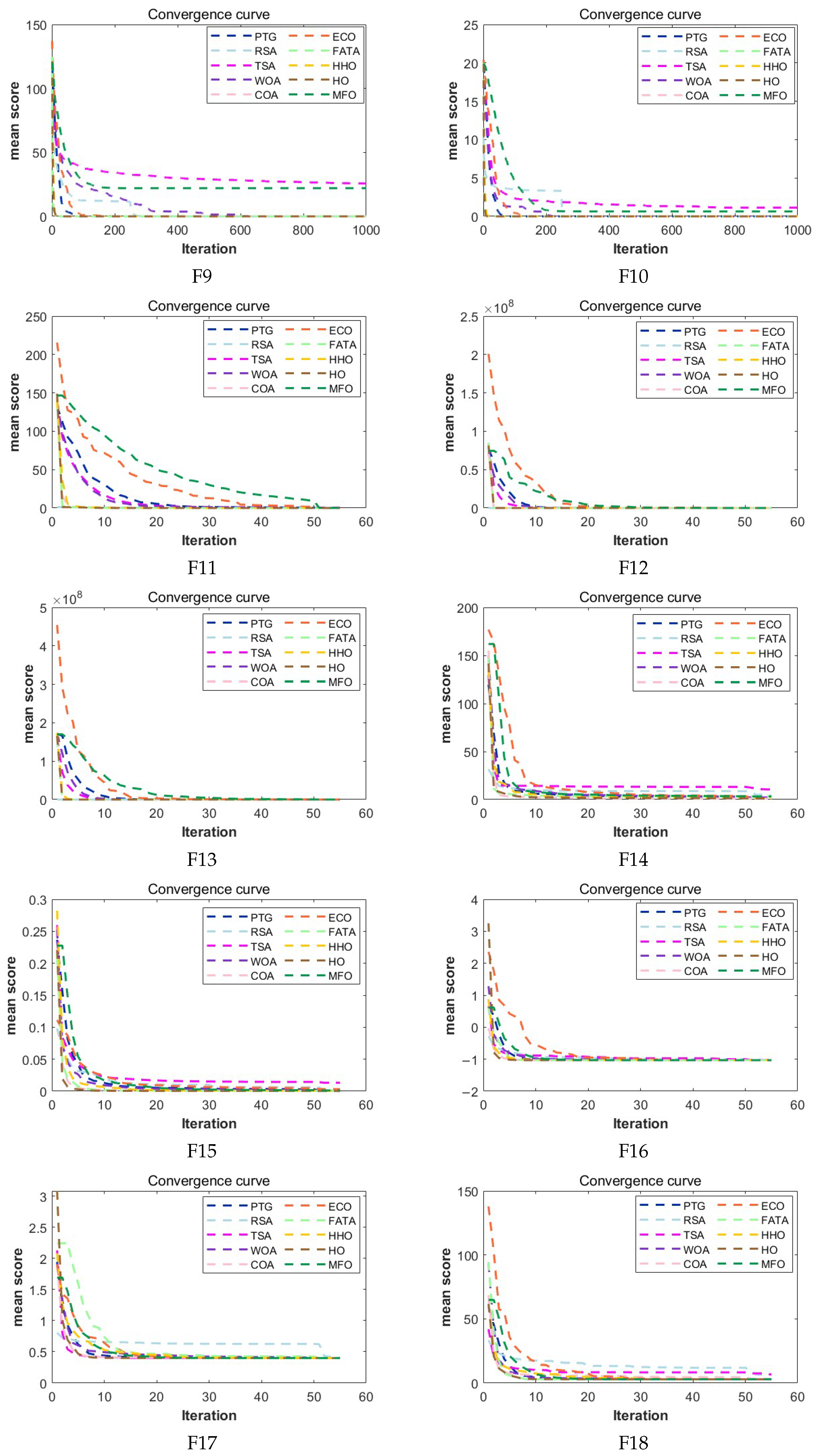
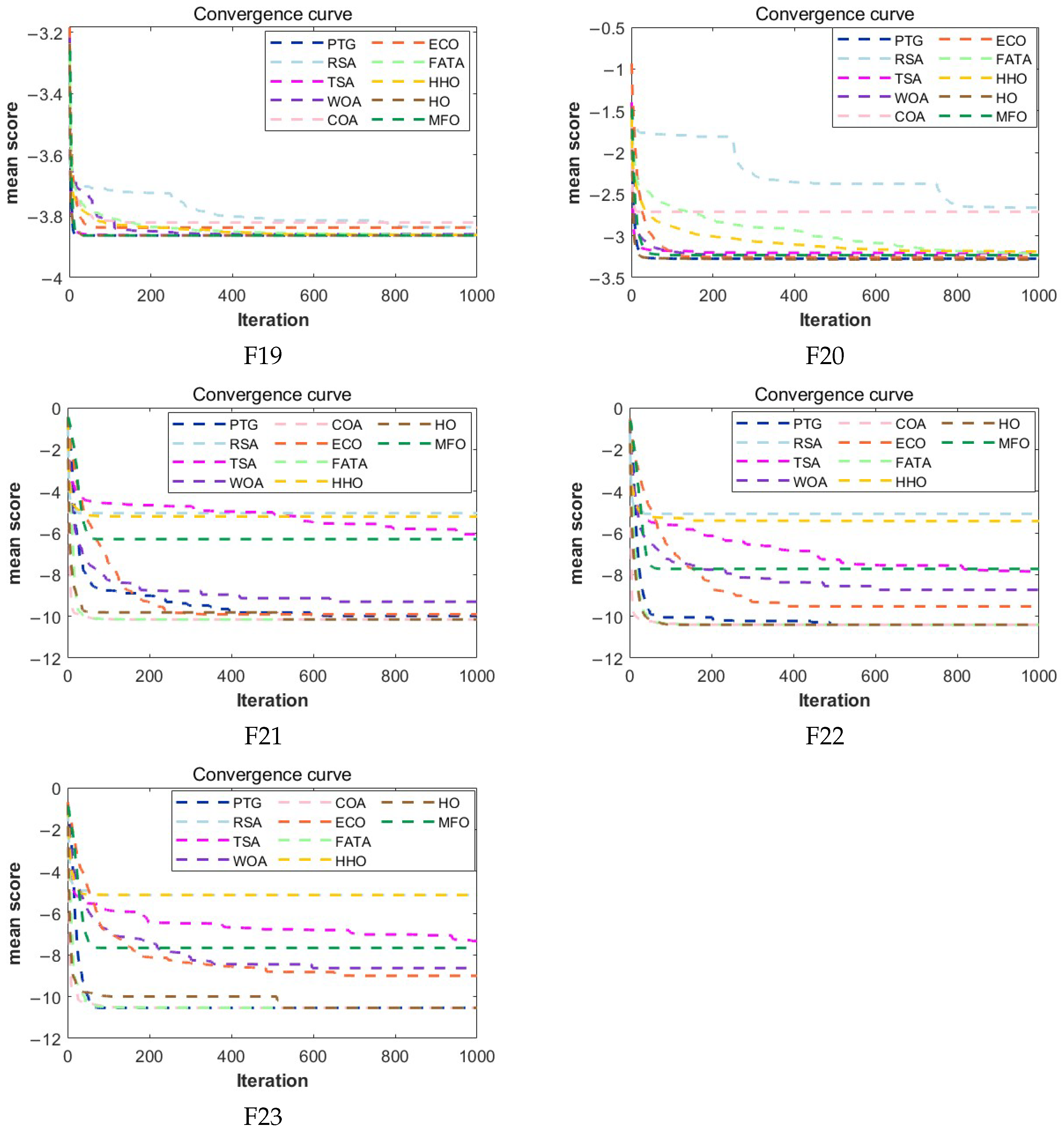
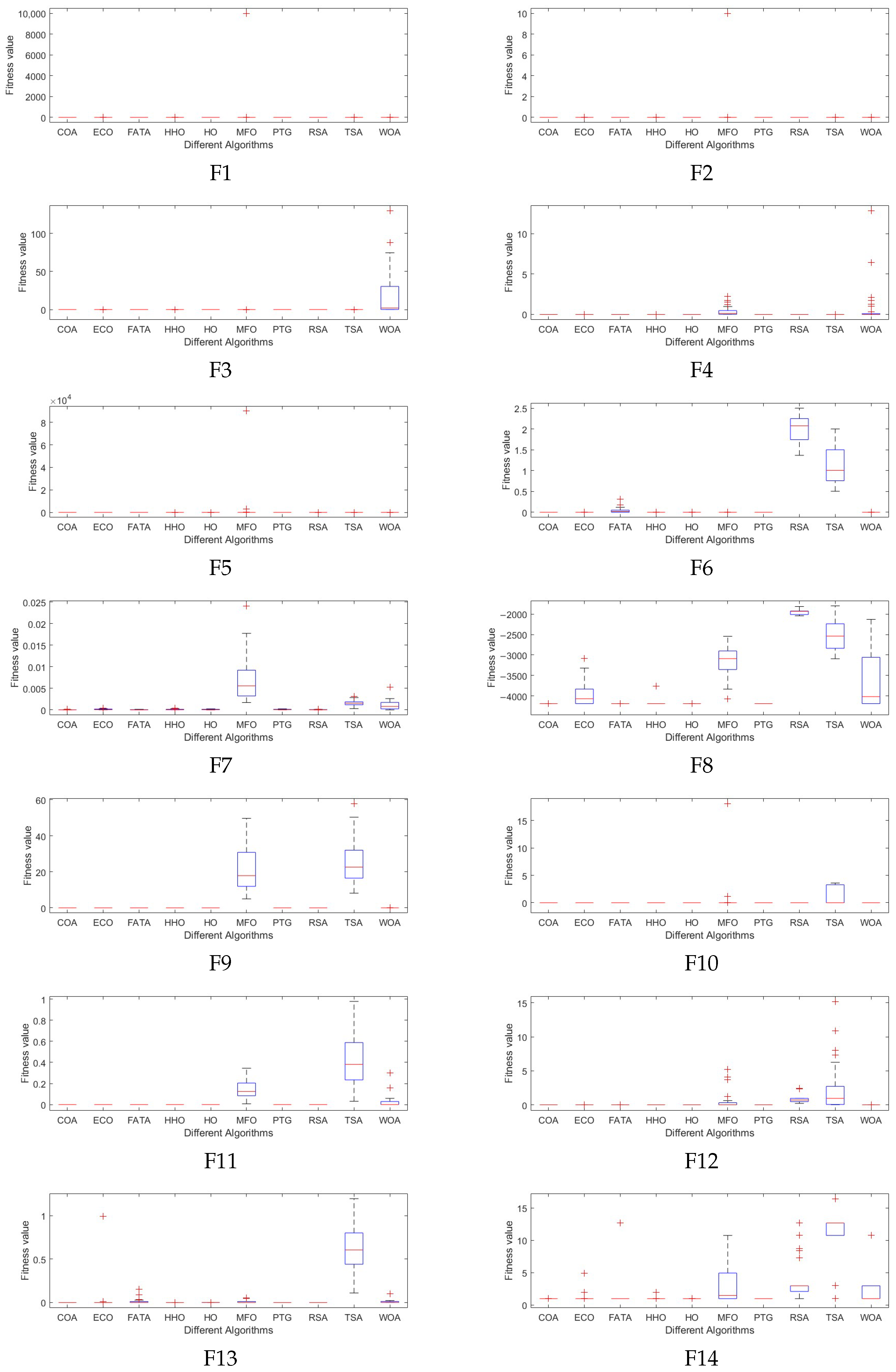
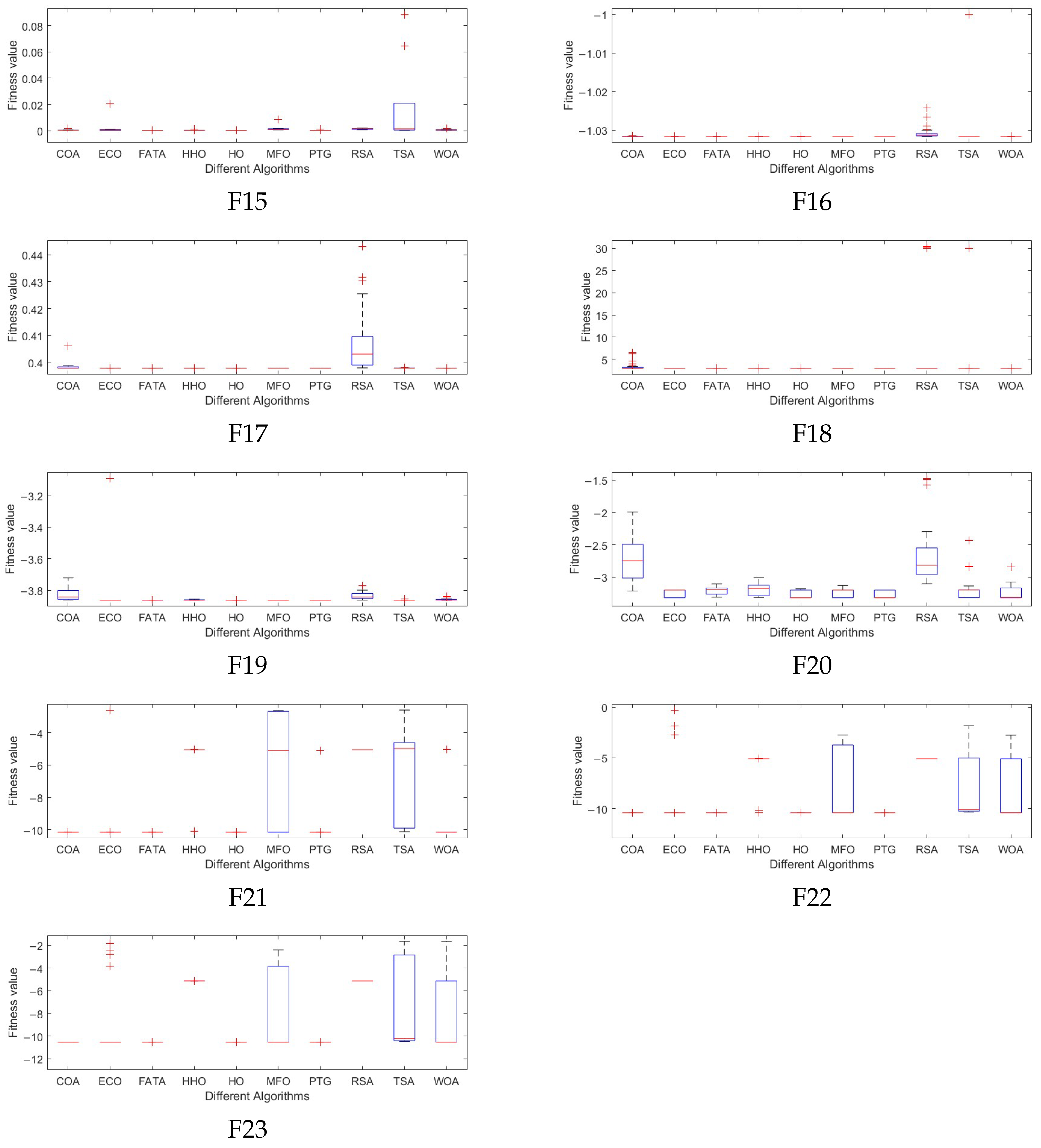
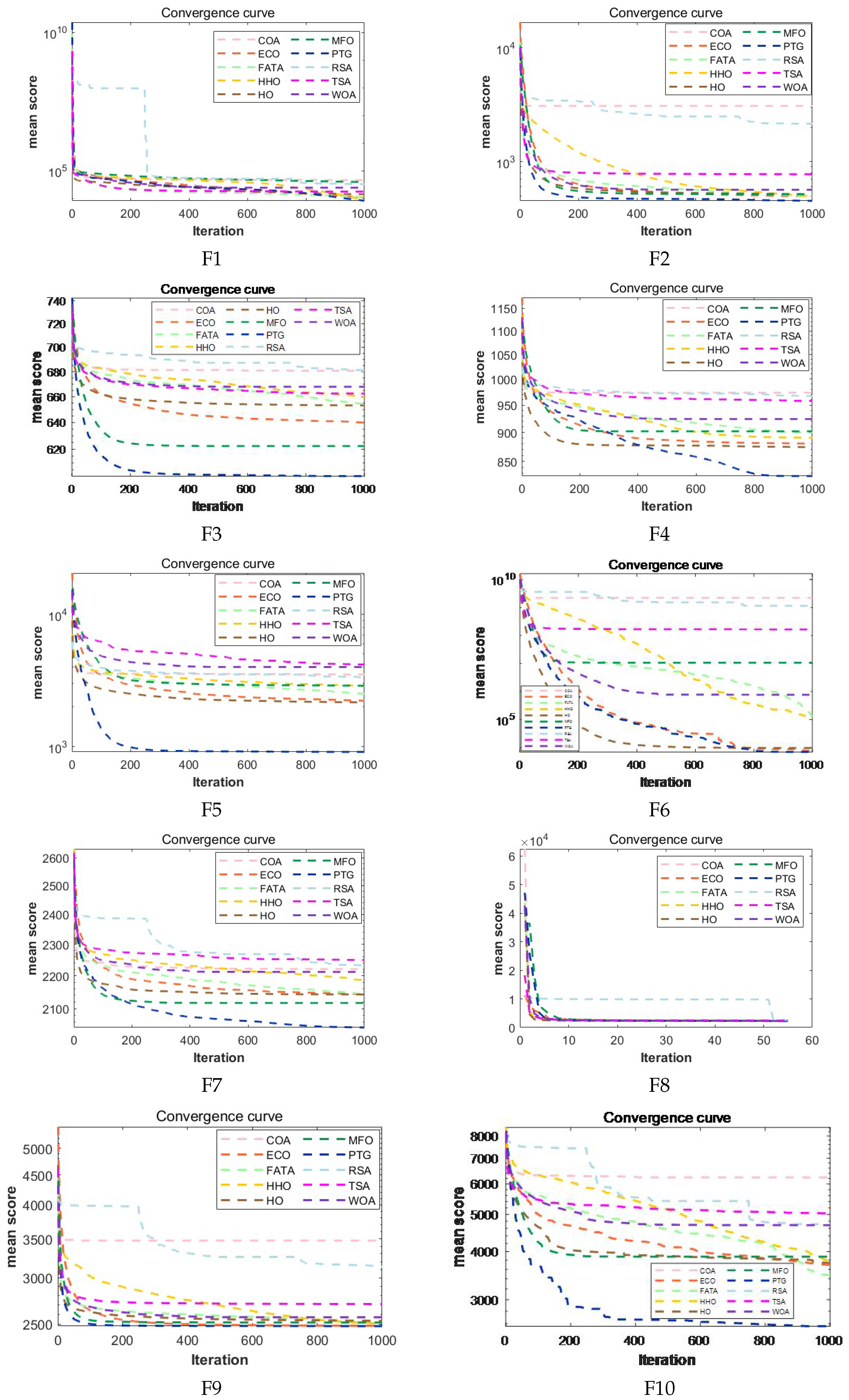
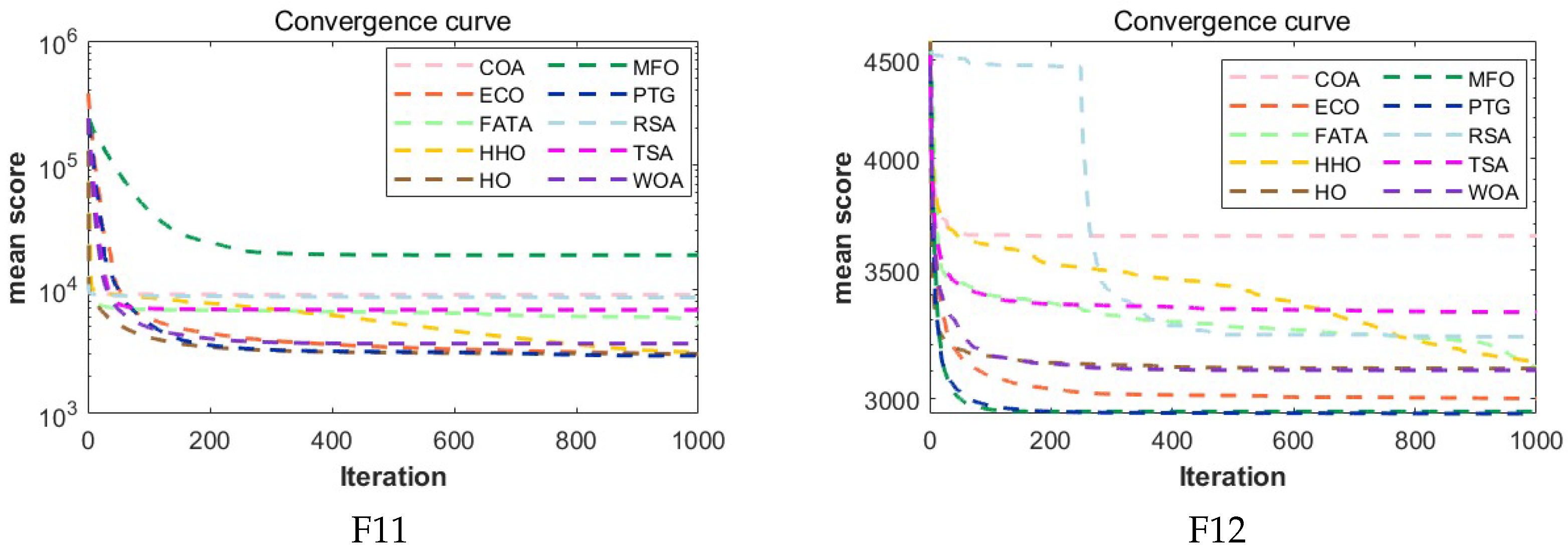
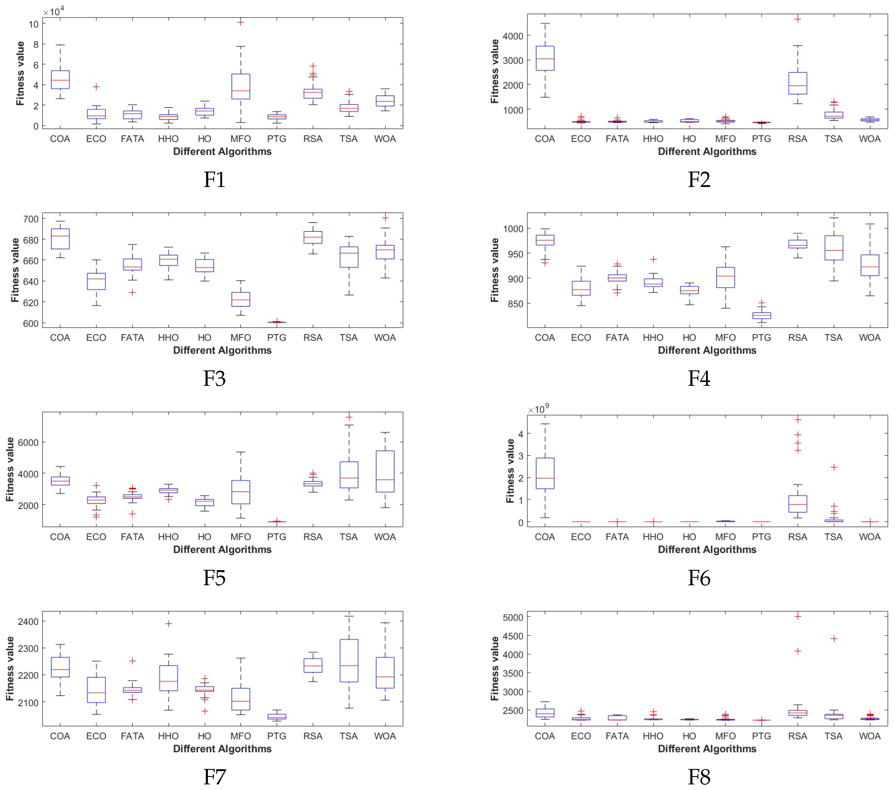
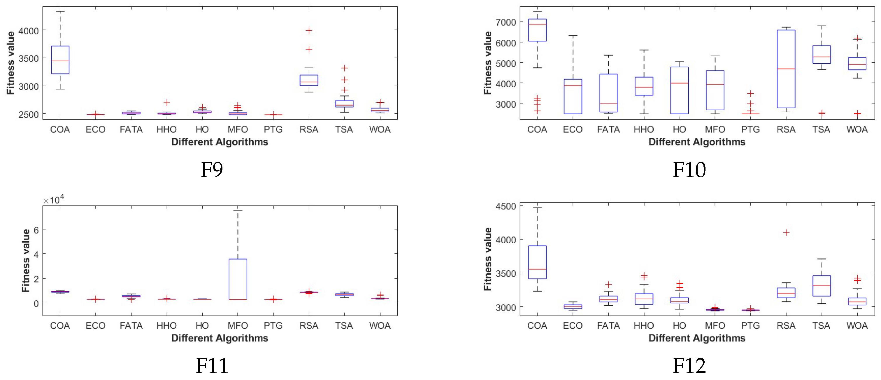
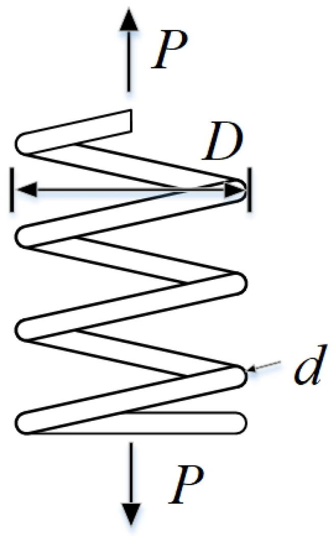
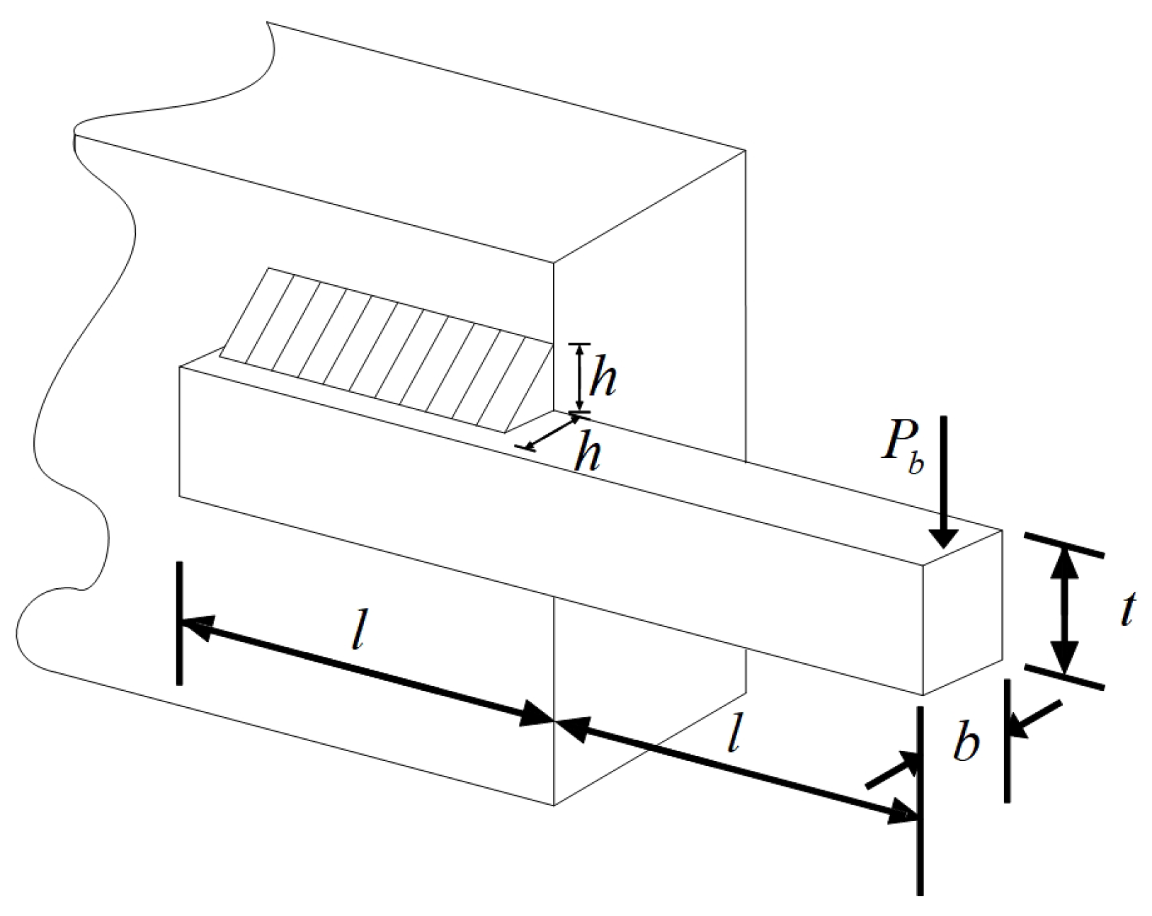
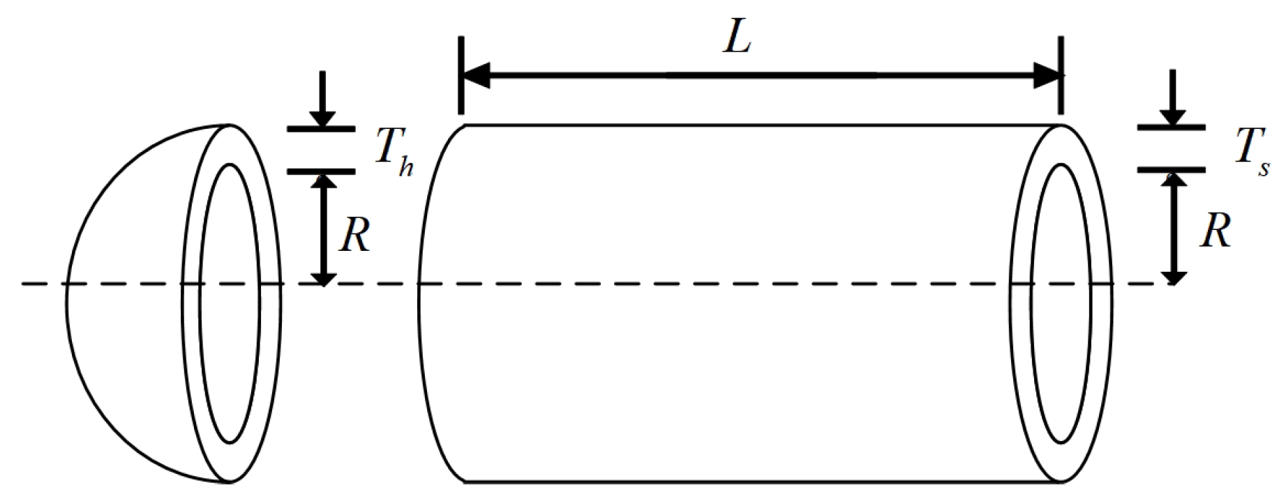
The experimental results show that compared with the other nine comparison algorithms, PTG performs best among 23 classical benchmark functions and CEC2022 benchmark functions, which shows that PTG is suitable for solving multimodal problems and unimodal benchmark functions with global convergence. In addition, PTG has solved four engineering problems, including spring compression design, welded beam structure, pressure vessel, and reducer design, which have practical application value. In addition, PTG ranks first in the Friedman test, which shows that PTG has obvious advantages in two different types of test functions. Although PTG has many advantages, there are still several limitations. Firstly, when dealing with high-dimensional data, the performance of PTG is similar to that of contrast algorithms, which indicates that the dimension distribution strategy requires a more comprehensive design to handle high-dimensional complex problems. Secondly, real-world problems are intricate and complex. For issues under complex constraints, the PTG algorithm may perform poorly, and all these need to be improved in future work. And in the future, we also plan to further expand the PTG algorithm to solve multi-objective optimization problems and use it to optimize large deep models.