A Novel Recognition-Before-Tracking Method Based on a Beam Constraint in Passive Radars for Low-Altitude Target Surveillance

Abstract

Effective means are urgently needed to identify non-cooperative targets intruding on airport clearance zones for the safety of low-altitude flights. Passive radars are an ideal means of low-altitude airspace surveillance for their low costs in terms of hardware and operation. However, non-ideal signals transmitted by third-party illuminators challenge feature extraction and target recognition in such radars. To tackle this problem, we propose a light-weight recognition-before-tracking method based on a beam constraint for passive radars. Under the background of sparse targets, the proposed method utilizes the continuity of target motion to identify the same target from the same array beam. Then, with its peaks detected in range-Doppler maps, a feature vector based on the biased radar cross-section is constructed for recognition. Meanwhile, to use the local scattering characteristics of targets for dynamic recognition, we introduce a parameter named normalized bistatic velocity to characterize the attitude of the target relative to the receiving station. With the proposed light-weight metric, the similarity of feature vectors between the unknown target and standard targets is measured to determine the target type. The feasibility and effectiveness of the proposed method are validated by the simulated and measured data.

1. Introduction

The surveillance and identification of low-altitude airspace targets is an important topic for civil aviation and general aviation. Due to the lack of effective methods, incidents of non-cooperative targets, such as unregistered aviation vehicles, drones, and balloons, intruding on airport clearance zones occur frequently, which pose severe threats to flight safety. In recent years, the rapid popularization of consumer-grade unmanned aviation vehicles (UAVs) has made the situation even worse. Since such targets generally have no responders, it is hard to identify them through automatic dependent surveillance broadcast (ADS-B) systems. Effective alternative means to distinguish them from civil and general aviation aircrafts around airports are urgently needed. Although active radars can achieve promising performance in target recognition by using features like micro-Doppler effects [1] and high-resolution range profiles (HRRPs) [2,3], their costs in terms of hardware and operation are too high for median and small airports. Low-cost means of low-altitude target surveillance are essential to improve flight support capability in such airports. Passive radars, which do not need transmitting systems, are an ideal candidate to satisfy this need. However, limited by the signal characteristics of third-party illuminators, such radars usually have the problem of low detection accuracy [4]. Consequently, the recognition performance of existing methods that depend on high-accuracy information provided by the detecting and tracking stages would be severely degraded in such radars and cannot satisfy the needs of real-life applications sufficiently. To facilitate the application of bistatic passive radars in various airports, we address the problem of recognizing non-cooperative targets under low detection accuracy in this paper. It is worth mentioning that previous signal processing methods, like beamforming and target detection, are not within the scope of this paper. Our study makes the basic assumption that the targets analyzed are well detected, but with low range and velocity accuracy.

Radio and television signals possess advantages like wide coverage and high transmission power, which make them an important illuminator of opportunity (IO) for passive radars. Extensive studies on passive radars based on such IOs have been made and reported in the field of low-altitude target surveillance [5,6,7,8]. Their promising results make passive radars an ideal means for the surveillance of low-altitude non-cooperative targets around airports. However, due to non-ideal characteristics of third-party illuminators, which are not designed for target detection, the quality of echo signals is not ideal to obtain high-resolution features like HRRPs and inverse synthetic aperture radar (ISAR) images. For example, the widely used digital television terrestrial multimedia broadcasting (DTMB) signal only has a bandwidth of 7.56 MHz [9], which is not wide enough to obtain high-resolution features. Although efforts have been made to use passive radars to obtain micro-Doppler features [10,11] and ISAR images [12] and recognize targets with passive radar images [13], it is still a challenge to achieve high performance in recognizing small air targets using such features due to the low signal-to-noise ratio and resolution. Thus, existing studies on target recognition with such radars mainly focus on low-resolution features like the radar cross-section (RCS) and track features [14,15,16,17,18]. In this paper, we seek to develop an effective and light-weight recognition method for bistatic passive radars based on the RCS.

In the existing literature, RCS-based target recognition studies mainly make use of the RCS for feature extraction and recognition in two ways. One of them is to extract the RCS through an electromagnetic simulation according to the measured track information. In this way, the incident angle and scattering angle of electromagnetic waves are first estimated from measured target tracks. And then the simulated target RCS is either calculated with a simulation model or looked up from a pre-calculated database [14,15]. Target recognition is usually realized by comparing a noisy received power profile to a simulated power profile computed from the simulated RCS [14]. These methods are validated through simulated data and show promising recognition performance. The other way is to construct a biased RCS by taking the unknown parameters as constants since they have no effect on the characteristic difference between different targets [16,17]. Recognizers are then built based on the constructed biased RCS. Their methods are validated through the synthetic dataset and measured dataset, and promising recognition results are achieved and reported. However, such promising recognition performance of the above studies is all based on the high-accuracy tracks provided by the previous processing, which makes the recognition performance heavily dependent on the tracking performance. For example, in reference [16], the feature vectors are constructed according to the order of the aspect angles and bistatic angles estimated from the measured tracks. Thus, when there are large errors in the target tracks, the simulated RCS or the extracted biased RCS, as well as the constructed feature vectors, would deviate severely from the true values. Consequently, the recognition performance would also degrade.

This problem shows a similar nature to the weak target detection in passive radars, where the target tracking is hindered by the difficult detection in the previous stage due to the weak target energy. To overcome the difficulty of detection and tracking caused by a weak signal-to-noise ratio in a single frame of data, a bunch of tracking-before-detection (TBD) methods are proposed [19,20]. They integrate signals from multiple frames and then backtrack target plots to realize tracking and detection simultaneously. Good results have been reported in the detection of weak targets like UAVs. Inspired by the TBD methods, it is a feasible way to alleviate the constraint of tracking error imposed on the recognition performance by preceding the recognition stage with the tracking stage. The joint tracking and classification (JTC) method is a potential strategy that would satisfy this purpose. In ref. [21], the authors propose a JTC method for a ground-based passive radar to obtain improved JTC performance. They introduce the simulated target RCS into the measurement vector to assist tracking. Promising performance from simulated data is obtained. However, the RCS calculation relies on the target position and attitude provided by the tracker. Thus, the performance of classification is still heavily dependent on the tracking performance. What is more, the deviation of simulated RCS from measured RCS would also make the method hard to apply in real situations.

To tackle the above problems, we propose a light-weight recognition-before-tracking (RBT) method based on a beam constraint for passive radars in this paper. To eliminate the side effects of tracking error imposed on the feature extraction, we move the construction of the feature vector and recognition ahead of track association. And by taking advantage of the continuity of target motion, we propose to take the targets detected in the same beam in a period of time as the same targets. On this basis, the target is detected, and its feature vector is constructed from multi-frame data of the same beam. Then, target recognition is realized using the biased RCS amplitudes and the corresponding time-varying characteristics from the angle of similarity measurement of the time series. The results from both simulated and measured data validate the feasibility and effectiveness of the proposed method for recognizing sparse targets with different feature sizes. The proposed method is suitable for the surveillance of non-cooperative targets at airports, especially for airports that cannot afford expensive active radars.

The main contributions of this paper are summarized as follows:

(1)

We propose a new method for feature vector extraction and construction based on a beam constraint. It extracts biased RCS from the detected peak on the range-Doppler (RD) map and takes targets from a short period of time in the same beam as the same target and constructs feature vectors accordingly. In this way, the target tracking is no longer needed for feature vector construction. Thus, it can sufficiently eliminate the side effects of tracking error imposed on the feature vector construction.

(2)

We propose a light-weight metric for measuring the similarity of feature vectors between the unknown target and standard targets. The metric is proposed based on the Euclidean distance (ED), trend consistency (TC), and volatility consistency (VC) of the feature vectors. Experimental results based on the simulated and synthetic data both validate its feasibility and effectiveness for recognizing targets with different feature sizes.

(3)

We propose a novel RBT method for passive radars. It utilizes the time sequence, extracted before target tracking from the biased RCS, to construct the feature vector of the unknown target. Meanwhile, the feature vectors of standard targets are dynamically constructed based on the attitude information of the unknown target. By measuring the similarity of feature vectors between the unknown target and standard targets, target recognition is realized. Experimental results show that the proposed method can make good use of the local scattering characteristics for effective target recognition.

The rest of this paper is organized as follows. Section 2 presents the key details of the proposed method. Section 3 shows the experimental results obtained from simulated and measured data. Section 4 discusses the recognition results and future works. The conclusions are drawn in Section 5.

2. Design of the Proposed Method

2.1. Block Diagram of the Proposed Method

The block diagram of the proposed light-weight RBT method is shown in Figure 1. It consists of the training stage and the recognition stage. Both stages are conducted in the array beam, which is formed using the conventional beamforming technique. During the training stage, the recognizer is trained in a supervised way. We first detect the cooperative targets from the RD map. Then, according to their true bistatic ranges and velocities, we extract their spectrum peaks, from which we estimate the biased RCSs for recognition. At the same time, we also estimate the attitude of targets relative to the receiving station according to the bistatic velocity and the central direction of the corresponding array beam. In this paper, we introduce a parameter, namely, the normalized bistatic velocity (NBV), to approximate the attitude of targets relative to the receiving station. To utilize the local RCS for recognition, the value range of this parameter is divided into several sub-sections. Then, we put the biased RCS into these NBV sub-sections in the target database accordingly. After obtaining all training data, we carry out a statistical analysis of the biased RCSs in each NBV sub-section. The resulting minimum value, mean value, and maximum value of biased RCSs are used to characterize the local scattering characteristics of the standard targets. These features from all NBV sub-sections constitute the model of the standard target of the proposed method.

During the recognition stage, we first obtain the detection results of unknown targets from the RD map. Then, we estimate a biased RCS and an NBV from each of the detected peaks. Based on the continuity of target motion, we take targets detected in a short period of time from the same array beam as the same targets and construct feature vectors from their biased RCSs. Meanwhile, an NBV time sequence is also constructed correspondingly. According to the NBV time sequence, we extract the corresponding biased RCS features from the standard target model and construct three types of standard feature vectors, i.e., the minimum value sequence (MIVS), the mean value sequence (MEVS), and the maximum value sequence (MAVS). Then, we calculate the ED, TC, and VC scores between feature vectors of the unknown target and the standard targets and then fuse them with pre-trained weights to obtain the primary fusion score. It should be mentioned that we use the reciprocal of ED but not its absolute value as the recognition score in terms of the feature distance in order to fuse it with the TC and VC scores. Finally, after fusing the primary fusion scores obtained from the three standard feature vectors with proper weights, we obtain a final recognition score (FRS). According to the maximum subordination principle, we assign the target type corresponding to the highest FRS as the one that the unknown target belongs to. Details about the proposed method will be introduced in the following sections.

2.2. Acquisition of Data and Construction of Standard Target Model

Passive radars operate on the signals emitted by third-party illuminators. Thus, the transmitting parameters are unknown. To avoid the influence of transmitting parameters on RCS estimation, reference [16] proposes a method that utilizes the reference signal to eliminate the transmitting parameters. It obtains an RCS estimation that is unrelated to the transmitting parameters by calculating the ratio of surveillance signal power to reference signal power at the receiving end. The resulting RCS estimation is as follows [16]:

$$\widehat{\sigma }={\displaystyle \frac{P_{rs}{G}_{rt}{(4\pi )}^3{R}_{ts}^2{R}_{rs}^2}{P_{rd}{G}_{rs}{\lambda }^{2}L}},$$

(1)

where $\widehat{\sigma }$ is the RCS estimation, $P_{rs}$ is the surveillance signal power, $G_{rt}$ and $G_{rs}$ are the gains of the reference antenna and the surveillance antenna, respectively, $R_{ts}$ and $R_{rs}$ are the distances of the target to the transmitting station and the receiving station, respectively, $P_{rd}$ is the reference signal power, $\lambda$ is the radar’s operating wavelength, and $L$ is the propagation loss of the reference signal. In conventional methods that recognize targets after tracking, a good RCS estimation can be obtained from (1). However, in the RBT problem, (1) is no longer applicable since $R_{ts}$ and $R_{rs}$ are unavailable.

The key issue in the RBT problem is that it is hard to obtain an accurate estimation of the direction of arrival (DOA) of the target signal before target tracking. In fact, we can only obtain a coarse estimation of the signal DOA according to the array beam direction. Thus, in our study, we use the central direction of the array beam to approximate the signal DOAs of the targets detected in it. Apparently, the narrower the beam width is, the more accurate this approximation is. On this basis, we utilize the relationship of $R_b=R_{ts}+R_{rs}$ and the parameter equation of the positioning ellipsoid to derive a biased estimation of the target RCS. The resulting estimation can be expressed as follows:

$${\widehat{\sigma }}_{bia}({\theta }_c,{\phi }_c)={\displaystyle \frac{\pi P_k{G}_{rt}{\left(R_b^2-R_{td}^2{\sin }^2{\theta }_c{\cos }^2{\phi }_c\right)}^2}{4G_p{P}_{rd}{G}_{rs}{R}_{td}^2{L}_{TER}}},$$

(2)

where ${\widehat{\sigma }}_{bia}({\theta }_c,{\phi }_c)$ is the biased estimation of target RCS, namely, the biased RCS, $({\theta }_c,{\phi }_c)$ is the direction angle of the equivalent beam center, which originates from the middle point of the baseline, $P_k$ is the amplitude of the target peak in the RD map, $R_b$ is the bistatic range of the target, $R_{td}$ is the baseline distance of the passive radar, $G_p$ is the signal processing gain, and $L_{TER}$ is the terrain loss for the reference signal propagating near the ground. It can be proven that the estimation error of this biased RCS is less than the RCS differences among UAV, general aviation aircraft (GAA), and civil aviation aircraft (CAA) targets. Thus, it would not affect the differences in scattering characteristics among these target types, which lays the foundation of using the biased RCS for target recognition.

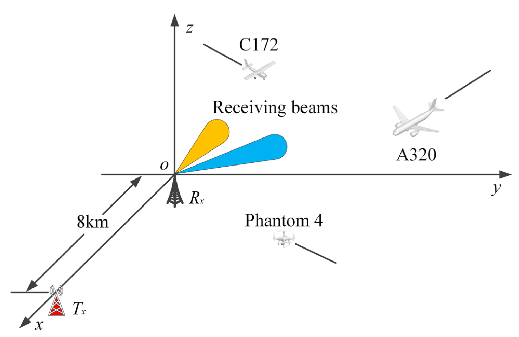
In this study, both simulated and measured data are used for validation of the proposed method. For the simulation validation, according to the application scenarios of the proposed method, we simulate a scene that contains targets of a CAA, a GAA, and a UAV simultaneously, as shown in Figure 2. The CAA is an A320 from Airbus, the GAA is a C172 from Cessna, and the UAV is a Phantom 4 from DJI (Shenzhen, China). Their feature sizes satisfy the following relationship: A320 > C172 > Phantom 4. Generally, the CAA and GAA are non-maneuvering targets and fly smoothly along their tracks. Thus, we simulate linear tracks for all targets in our study. For each target type, we randomly generate 150 tracks, each 50 points long. The direction of these tracks satisfies the uniform distribution in the range of [0, 2π]. And according to the velocities of these targets in real situations, we limit the value ranges of velocities of A320, C172, and Phantom 4 to [100, 150] m/s, [50, 65] m/s, and [10, 30] m/s, respectively.

From the generated tracks, we pick two-thirds of them as the training dataset and the remaining one-third as the testing dataset. The training dataset is used to construct the standard target model and train the weights for fusion of recognition features and statistical features. The testing dataset is used to evaluate the performance of the proposed method.

In the simulation scenario, we simulate a bistatic passive radar with a baseline distance of 8 km. As shown in Figure 2, the radar coordinate system originates at the receiving station, and the transmitting station is located in the east direction of the receiving station. In our study, the signal DOA of the target is estimated coarsely according to the central direction of the array beam, which is also used as the constraint to differentiate different targets under a sparse target background. That is, we take the targets detected in a short period of time in the same beam as the same target and construct feature vectors accordingly. With the simulated tracks, bistatic RCS of targets, and the configuration of the simulated passive radar, the received target echo power is generated accordingly. Finally, the biased RCS is extracted according to Formula (2).

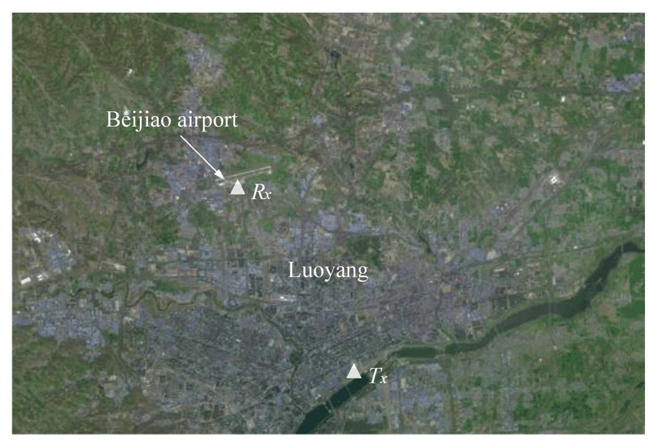
For the measured data validation, historical measured data provided by the Radio Detection Center of Wuhan University is used. The data used is collected with the multistatic passive radar developed by Wuhan University in 2019 at Beijiao Airport of Luoyang City, Henan Province, China, as shown in Figure 3. The illuminator of opportunity used in the field experiment is a television station that transmits DTMB signals. There are mainly two types of planes contained in the observation data, i.e., the A320 and the Cirrus SR20. It is worth mentioning that the SR20 has similar feature sizes to the C172, which is used in the simulation. All measured targets are confirmed through the ADS-B system.

In China, UAV flights are forbidden in the vicinity of airports. Thus, we cannot collect observation data of UAVs in such scenarios. To obtain the observation data containing the CAA, GAA, and UAV simultaneously, we generate the echo data of the UAV with the simulated Phantom 4 model and synthesize them with the measured data. The results shown in the measured data validation section are all obtained with the synthetic data. Similarly to the simulation data, we divide the synthetic data into two sets. The first two-thirds of them are used as the training data, and the remaining one-third is used as the testing data.

In our study, the recognition feature used for target recognition is constructed from the biased RCS. Specifically, it is the biased bistatic RCS, which is the true bistatic RCS attached with a small deviation induced by the unknown position, in the detection scenario of passive radars. Thus, the characteristic difference in the true bistatic RCS between different target types is the foundation of utilizing the biased bistatic RCS for recognition. In this section, we will investigate the characteristic difference in the bistatic RCS between the three simulated targets.

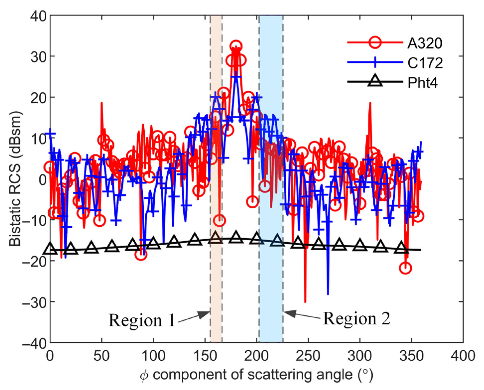
Under the scenario shown in Figure 2, we set the $\theta$ component and $\phi$ component of the incident angle (denoted as ${\theta }_{inc}$ and ${\phi }_{inc}$, respectively) to 93° and 0°, respectively, and those of the scattering angle (denoted as ${\theta }_{sca}$ and ${\phi }_{sca}$, respectively) to 93° and 0° ≤ ${\phi }_{sca}$ ≤ 359°, respectively. The resulting bistatic RCSs of the A320, C172, and Phantom 4 are shown in Figure 4. It should be noted that Pht4 in the legend denotes the Phantom 4. The results in Figure 4 show that the peak value of the bistatic RCS of the A320 is the largest, and that of the Phantom 4 is the smallest, which shows the same relationship as that between their feature sizes.

However, although the feature sizes of the A320 are greatly larger than those of the C172, the value ranges of their bistatic RCS overlap evidently with each other, according to the results shown in Figure 4. For example, the bistatic RCSs of A320 in region 1 have the same amplitudes as those of the C172 in region 2. Similar phenomena can also be observed in other angle regions. As a result of this, the bistatic RCSs of these two target types are not very distinguishable from their amplitude, which would lead to poor recognition performance. Nevertheless, we can further find that their bistatic RCSs corresponding to the same angle region show an obvious difference in the amplitude. Thus, it is feasible to differentiate these two target types from the local bistatic RCS. And this is exactly the foundation of the proposed method in this paper.

Based on the above analysis, we introduce a parameter, namely, the NBV, to characterize the attitude of targets relative to the receiving station. With the help of the NBV, we can make full use of the RCS difference between different targets in the local angular range for recognition. For this purpose, we first divide its value range into multiple sub-sections to realize the analysis of local scattering characteristics and the extraction of local RCS features of the target. The NBV is defined and calculated as follows:

$$v_{NBV}\triangleq \cos \delta ={\displaystyle \frac{{\widehat{v}}_b}{{\widehat{v}}_{b,\max }}},$$

(3)

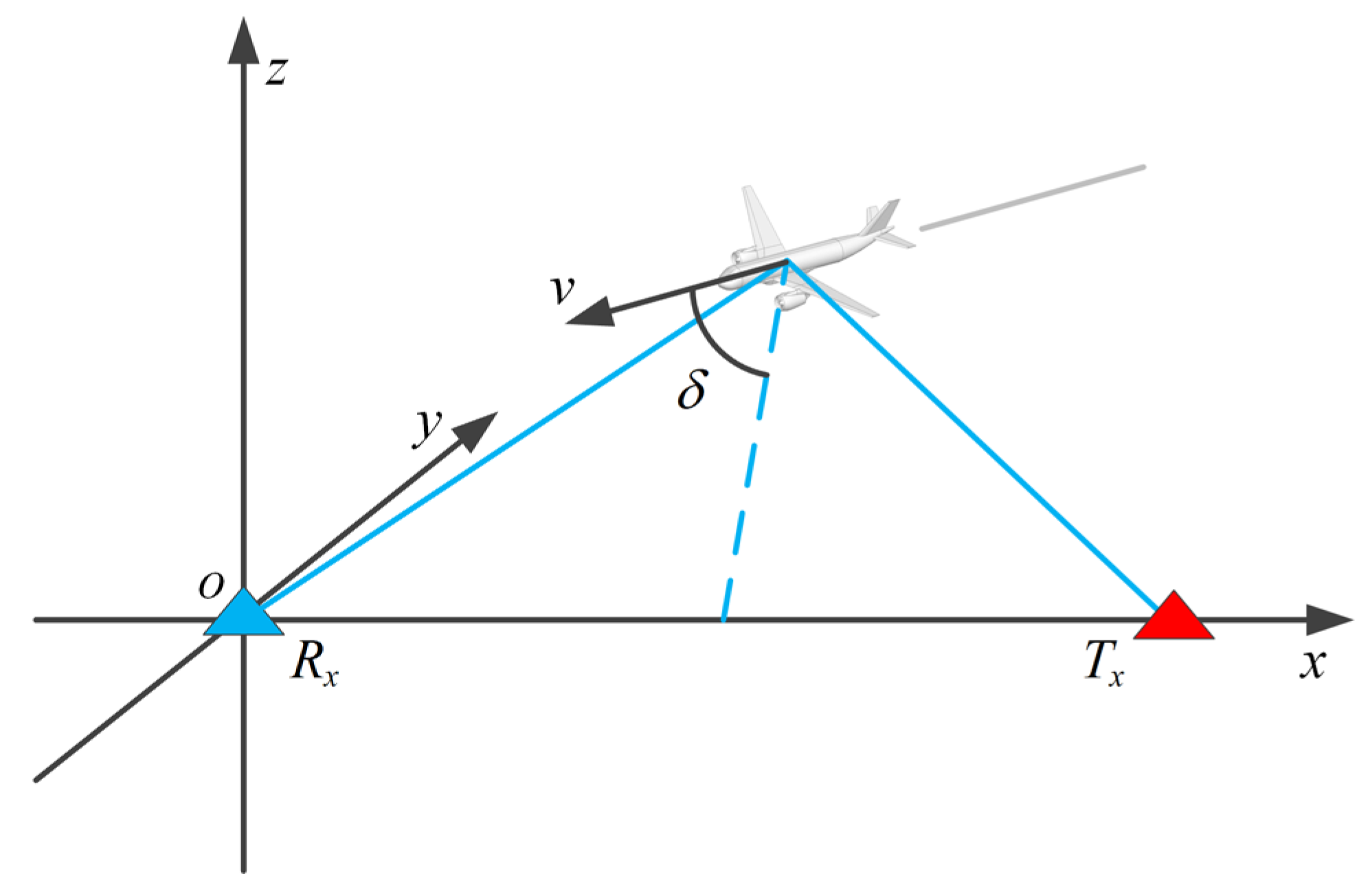
where $\delta$ is the angle between the velocity direction of the target and the bisector of the bistatic angle, ${\widehat{v}}_b$ is the biased bistatic velocity, and ${\widehat{v}}_{b,\max }$ is the maximum value of the biased bistatic velocity obtained from the training data. The ${\widehat{v}}_b$ is calculated as follows:

$${\widehat{v}}_b={\displaystyle \frac{\lambda f_d}{2\cos ({\beta }_{est}/2)}},$$

(4)

where $f_d$ is the Doppler frequency of the target, and ${\beta }_{est}$ is the biased estimation of the bistatic angle and is expressed as follows:

$${\beta }_{est}=\left\{\begin{array}{l}{\displaystyle \frac{R_b^2-R_{td}^2}{2(R_b+R_{td}\sin {\phi }_r)}}, {\phi }_r<0\\ {\displaystyle \frac{R_b^2-R_{td}^2}{2(R_b-R_{td}\sin {\phi }_r)}}, \mathrm{else}\end{array}\right.,$$

(5)

where ${\phi }_r$ = $\pi /2$ − ${\phi }_c$. It can be seen from (3) and (4) that the NBV is related to $\delta$. Figure 5 shows the relationship between $\delta$ and the target velocity. It can be seen that the facet of the target facing the receiving station is closely related to $\delta$. Generally, the plane targets have an axisymmetric shape. In our study, we take the symmetrical parts as the same one and thus can obtain a one-to-one relationship between the target facet facing the receiving station and the $\delta$ angle. Based on this relationship, we can obtain a coarse estimation of the target attitude relative to the receiving station through the NBV. It is worth mentioning that the NBV is valid only when the velocity direction coincides with the orientation of the target. Otherwise, it would fail to approximate the target attitude relative to the receiving station since the $\delta$ angle cannot accurately reflect the facet of the target facing the receiving station through its value.

Then, we divide the value range of NBV into multiple sub-sections. In each NBV sub-section, we make a statistical analysis on the training data of biased RCS and obtain three statistical features, which are the minimum value, mean value, and maximum value of the local biased RCSs. They are expressed as follows:

$${\widehat{\sigma }}_{MIVS}=\underset{n\in [1,N]}{\min }({\widehat{\sigma }}_{bia,n}),$$

(6)

$${\widehat{\sigma }}_{MEVS}={\displaystyle \frac{1}{N}}{\displaystyle \sum _{n=1}^N{\widehat{\sigma }}_{bia,n}},$$

(7)

$${\widehat{\sigma }}_{MAVS}=\underset{n\in [1,N]}{\max }({\widehat{\sigma }}_{bia,n}),$$

(8)

where the ${\widehat{\sigma }}_{MIVS}$, ${\widehat{\sigma }}_{MEVS}$, and ${\widehat{\sigma }}_{MAVS}$ are the minimum value, mean value, and maximum value of the local biased RCSs, respectively, and N is the number of biased RCSs in an NBV sub-section. These statistical features are used to characterize the local scattering characteristics of the standard targets in a small angle range.

2.3. Construction of Feature Vector of Unknown Targets Under Beam Constraint

In real scenarios, the non-cooperative targets are usually sparse in the vicinity of airports. This allows a radar to distinguish them with different beams. Under this condition and the continuity of target motion, we propose to take the targets detected in the same beam in a short period of time as the same target in this study. Thus, we are able to construct feature vectors of unknown targets before tracking.

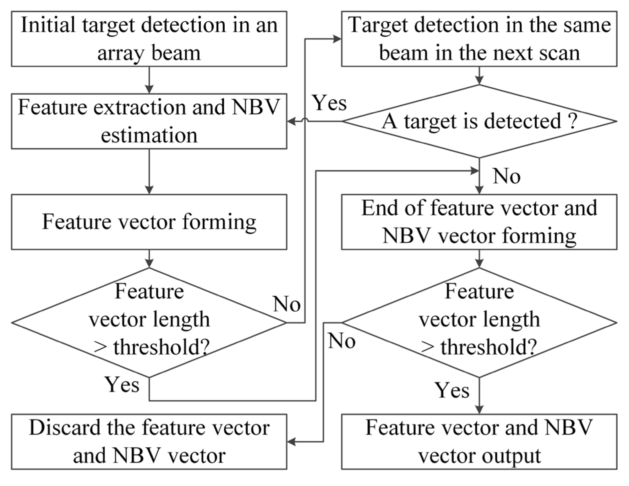
The flow diagram of the proposed method of feature vector construction in our study is shown in Figure 6. It starts when a target is detected in an array beam. Under such circumstances, we extract the biased RCS and NBV from the peak in the RD map using the method introduced in Section 2.2. Then, we move to the next scan of data to check whether or not there is still a target in the same beam. We continue to construct a feature vector with the newly extracted biased RCS and NBV from the newly detected peak until there are no targets detected in the new data or the length of the feature vector reaches the threshold. Then, the feature vector is output for further processing when its length satisfies the threshold. It is worth mentioning that under the assumption of sparse targets in the detection scenario, it is reasonable to assume that an array beam contains only one target. Under such circumstances, the strongest peak is considered the target in case of multiple detected peaks induced by false alarms.

Assuming that the biased RCS and NBV extracted from the target peak detected in the m-th array beam are ${\widehat{\mathit{\sigma }}}_{bia}^{(m)}$ and ${\mathit{v}}_{NBV}^{(m)}$, respectively, then the constructed feature vector and NBV vector can be expressed as follows:

$${\widehat{\mathit{\sigma }}}_{bia}^{(m)}= {({\widehat{\sigma }}_{bia,1}^{(m)}, {\widehat{\sigma }}_{bia,2}^{(m)}, \dots , {\widehat{\sigma }}_{bia,N_f}^{(m)})}^{\mathrm{T}},$$

(9)

$${\mathit{v}}_{NBV}^{(m)}={(v_{NBV,1}^{(m)}, v_{NBV,2}^{(m)}, \dots , v_{NBV,N_f}^{(m)})}^{\mathrm{T}},$$

(10)

where ${\widehat{\mathit{\sigma }}}_{bia}^{(m)}$ and ${\mathit{v}}_{NBV}^{(m)}$ denote the biased RCS vector and NBV vector, respectively, and $N_f$ denotes the vector length.

It should be mentioned that when there are multiple targets detected in multiple beams, we separate these targets according to the beam indices and construct feature vectors and NBV vectors for them.

2.4. Dynamic Recognition with Time-Varying Feature Vector

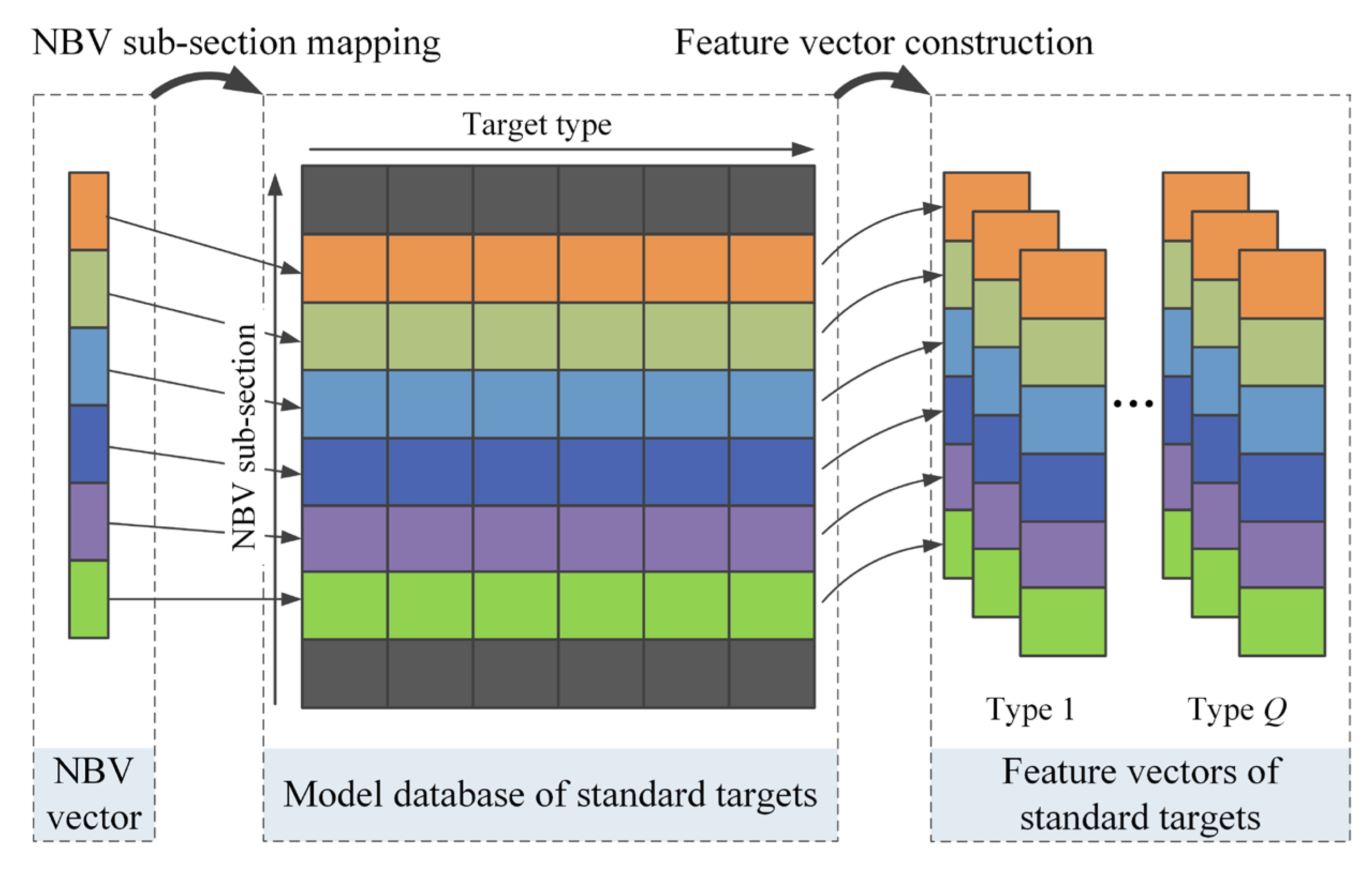
In this section, we realize target recognition by measuring similarity between feature vectors of the unknown target and standard targets. Unlike conventional pre-trained recognition methods, the standard target model, i.e., the standard feature vector, used in our study, is dynamically constructed according to the NBV vector estimated from the unknown target. As shown in Figure 7, we first extract statistical features of standard targets from the target model database to construct standard feature vectors according to the NBV vector of the unknown target. Since the values in the NBV vector indicate the NBV sub-sections corresponding to the biased RCSs in the feature vector of the unknown target, the constructed standard feature vectors reflect the same local characteristics as those of the unknown target. Then, by arranging these features according to the order of NBV values in the NBV vector, we obtain three feature vectors corresponding to the minimum value, mean value, and maximum value of the biased RCS for each standard target.

Assuming that the three constructed feature vectors corresponding to the q-th standard target are ${\widehat{\mathit{\sigma }}}_{MIVS}^{(q)}$, ${\widehat{\mathit{\sigma }}}_{MEVS}^{(q)}$, and ${\widehat{\mathit{\sigma }}}_{MAVS}^{(q)}$, respectively, then the similarity between the unknown target and standard targets will be measured through the comprehensive similarity between them. In essence, the feature vector can be regarded as a kind of time sequence. In published studies in the literature, there are numerous metrics for similarity measurement between time sequences, such as the ED [22,23], dynamic time warping (DTW) [24,25,26,27], and set-based similarity [28]. However, the ED and the set-based similarity suffer from noise and, hence, are not robust enough. The DTW is elastic in time shifting and effective in most scenarios. However, it suffers from a large computational burden when the length of the time sequence increases. Thus, to realize light-weight but robust similarity measurement, a new metric needs to be developed.

According to the differences in feature amplitude and feature vectors’ inside trend and volatility among different target types, we construct a new metric to measure the similarity of feature vectors between the unknown target and standard targets based on the ED, TC, and VC jointly, which is expressed as follows:

$$s_{\ast }^{(q)}=w_1{s}_{d,\ast }+w_2{s}_{TC,\ast }+w_3{s}_{VC,\ast },$$

(11)

where * denotes the feature type, i.e., the MIVS, the MEVS, and the MAVS; $s_{\ast }^{(q)}$, namely the proposed similarity metric, denotes the fusion score of the unknown target relative to the q-th standard target in terms of the statistical feature represented by *; $s_{d,\ast }$, $s_{TC,\ast }$, and $s_{VC,\ast }$ are the recognition scores corresponding to the ED, TC, and VC in terms of the feature ‘*’, respectively; and $w_1$, $w_2$, and $w_3$ are the weights for fusing them. The effectiveness of the proposed similarity metric has been validated through simulated data, which shows that the resulting recognition performance is the best when the ED, TC, and VC are considered simultaneously.

The score corresponding to the ED, namely, the distance recognition score (DRS), is defined as follows:

$$s_{d,\ast }={\displaystyle \frac{1}{{‖{\widehat{\mathit{\sigma }}}_{\ast }^{(q)}-{\widehat{\mathit{\sigma }}}_{bia}^{(m)}‖}_2}},$$

(12)

where ${\widehat{\mathit{\sigma }}}_{\ast }^{(q)}$ denotes the feature vector of the q-th standard target in terms of the feature ‘*’. The denominator in (12) is the ED. We use the reciprocal of the ED as the DRS based on the ground truth that the more similar the unknown target is to the standard target, the smaller the distance between their feature vectors. Thus, the more similar the unknown target is to the standard target, the higher the DRS.

The recognition score corresponding to the TC is defined according to the varying trend in the features inside the feature vector. Since the biased RCS varies non-linearly with the NBV sub-section, we measure the TC between two feature vectors, one segment by one segment. Thus, the score of TC, namely the TC score (TCS), is calculated as follows:

$$s_{TC,\ast }=N_{sm,\ast }/N_{seg,\ast },$$

(13)

where $N_{seg,\ast }$ and $N_{sm,\ast }$ are the total segments of the feature vector curve and the number of segments that have the same direction, respectively.

In the field of statistics, the standard deviation is the index that is used to characterize the volatility of data. On this basis, we construct a parameter, namely the VC score (VCS), to characterize the volatility of features inside the feature vector as follows:

$$s_{VC,\ast }=1-{\displaystyle \frac{\left|{\sigma }_{std,\ast }-{\sigma }_{unk,\ast }\right|}{{\sigma }_{std,\ast }+{\sigma }_{unk,\ast }}},$$

(14)

where ${\sigma }_{std,\ast }$ and ${\sigma }_{unk,\ast }$ are the standard deviations of features in the feature vector of the standard target and the unknown target, respectively. Substituting the three feature vectors of the standard target into (11)–(14), we obtain three primary fusion scores corresponding to them, which are expressed as follows: $s_{MIVS}^{(q)}$, $s_{MEVS}^{(q)}$, and $s_{MAVS}^{(q)}$.

It is worth mentioning that in our study, we use three statistical features of the biased RCS to measure the similarity between the unknown target and the standard target. The main reason is that the feature vector of the unknown target is a result estimated from multiple scans of data in a short period of time. Since it is not a statistical result, the values in the feature vector fall into the range defined by the minimum value and the maximum value. Thus, the characteristics reflected by the feature vector of the unknown target are moderate ones between those reflected by the minimum value and the maximum value. Under such circumstances, it is not appropriate to use only the feature vector of the minimum value, the mean value, or the maximum value of the biased RCS to recognize the unknown target. Instead, it is better to comprehensively take all three types of feature vectors to measure the similarity between the unknown target and the standard target. Thus, we further fuse the recognition scores corresponding to the three types of feature vectors with proper weights to obtain the final recognition score, i.e.,

$$s_q=w_4{s}_{MIVS}^{(q)}+w_5{s}_{MEVS}^{(q)}+w_6{s}_{MAVS}^{(q)},$$

(15)

where $s_q$ is the FRS of the unknown target relative to the q-th standard target, and $w_4$, $w_5$, and $w_6$ are the pre-trained fusion weights for the $s_{MIVS}^{(q)}$, $s_{MEVS}^{(q)}$, and $s_{MAVS}^{(q)}$, respectively.

After comparing the feature vector of the unknown target to those of the standard targets in the database, we obtain a final recognition score relative to each of them, which can be expressed as s = ($s_1$, $s_2$, …, $s_q$)^T. Then, the target type of the unknown target can be determined according to the maximum subordination principle, i.e.,

$$j=\underset{q\in [1,Q]}{\arg \max }(s_1, s_2, \dots , s_q),$$

(16)

where j denotes the index of the target type that the unknown target belongs to.

In our study, all of the above weights are trained with the training data. Since there are no explicit constraints for these weights, we use the particle swarm optimization (PSO) algorithm, which is the algorithm that is widely used in unconstrained optimization problems, to train them. Details about the realization of the PSO algorithm can be found in [17]. Moreover, it can be inferred from the above derivation that the computational complexity of the proposed method is only O(3$N_f$ + 8), which is significantly less than that of the DTW method, which possesses a computational complexity of O($N_f^2$), when $N_f$ is a large value. Thus, when the length of the feature vector increases to a large value, the computational burden will not increase significantly. What is more, the number of coefficients used in the proposed method is only 6, which is significantly less than that used in the neural network-based methods. Thus, the proposed method is more light-weight and easier to train. This is the main reason that we call the proposed method a light-weight one.

3. Simulation and Measured Data Results

The proposed method is currently in the stage of laboratory development and testing. Real-life use will be implemented after adequate testing with simulated data and measured data collected historically. In this section, validation results obtained from simulated data and measured data are presented.

3.1. Performance Evaluation of the Proposed Method Under Different Beam Widths

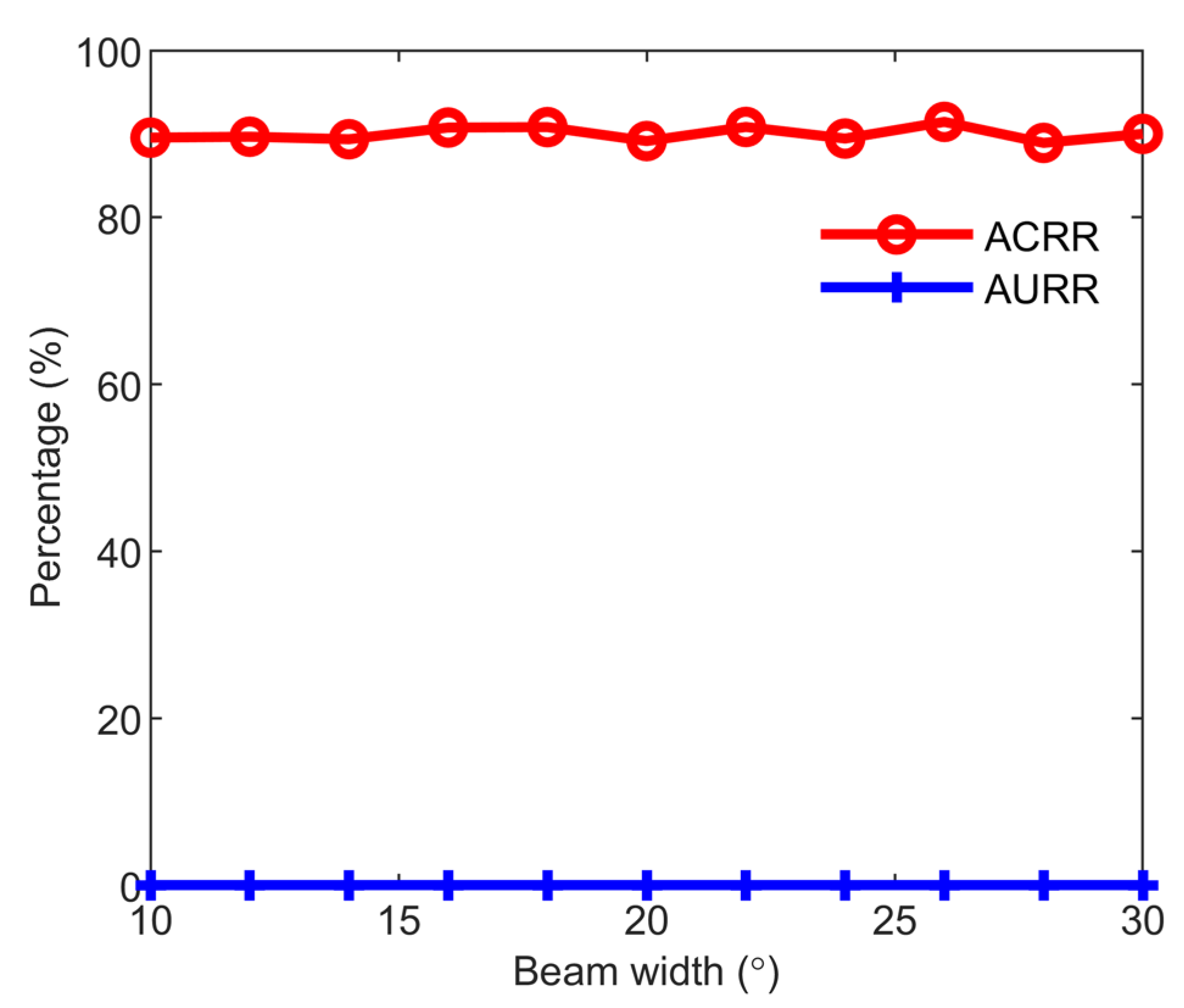
In our method, the array beam is the constraint of constructing feature vectors, and its central direction is used as the approximation of the signal DOA of the target. Thus, beam width is a key parameter that determines the accuracy of feature vector construction and attitude estimation. This section investigates the influence of this parameter on the performance of the proposed method. We conduct a series of recognition experiments by varying the beam width in the range of [10°, 30°] with a step of 2° and calculate the average correct recognition rates (ACRRs) and the average unknown recognition rates (AURRs) correspondingly. The results are shown in Figure 8. It is worth mentioning that the feature vector length used in all recognition experiments is 20.

It can be seen from the red curve that the ACRR fluctuates around 90% when the beam width increases. At the same time, the AURR remains unchanged and is always 0%, as shown in the blue curve. These results indicate that the performance of the proposed method is insensitive to the beam width in the range of [10°, 30°]. Thus, the proposed method is suitable for use in passive radars with narrow array beams since its performance is robust under such circumstances. The main reason for this phenomenon is that the differences in bistatic RCS among the three simulated targets are greatly larger than the estimation error of biased RCS induced by the beam width, even if it reaches 30°. Thus, although the estimation error of the biased RCS increases with the increasing beam width, it is still less than the difference in bistatic RCS among the targets and will not affect the recognition. However, there is still fluctuation on the ACRR curve since the varying beam width will change the direction of the beam center, which will further change the estimation of the NBV. Since the biased RCSs obtained from the training dataset are divided into different NBV sub-sections according to the corresponding NBV values, the resulting standard target models in the NBV sub-sections vary accordingly. Although such variation is mild under different beam widths, it will still change the final ACRR. Thus, the ACRR fluctuates when the beam width increases.

3.2. Performance Evaluation of the Proposed Method Under Different Lengths of Feature Vectors

The feature vector is a short time sequence that depicts the trend in the biased RCS of targets varying with the attitude. Its length determines the amount of information to be used for recognition, which is another key factor that determines the performance of the proposed method. In this section, we investigate the influence of this parameter on the ACRR and AURR of the proposed method. The conclusions found in this section will be of great value to the determination of the feature vector length in real-life applications.

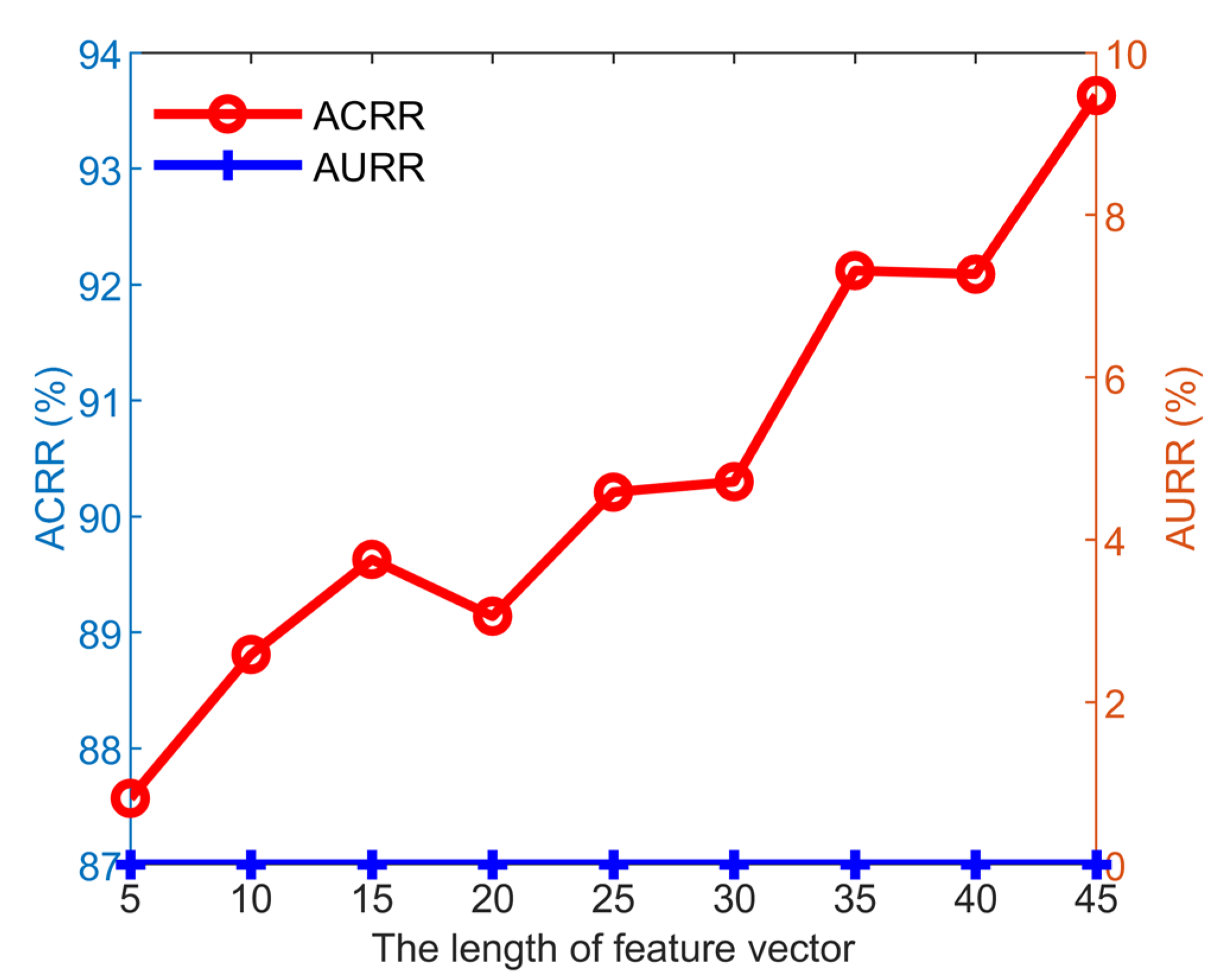
In the recognition experiments, we vary the feature vector length in the range of [5, 45] with a step of 5 and fix the other parameters. The resulting ACRR and AURR curves versus the feature vector length are shown in Figure 9. It can be seen that the AURR remains unchanged with the value of 0% whereas the ACRR fluctuates and rises when the feature vector length increases. It is easy to understand the increment of the ACRR since more information is used for recognition when the feature vector length increases, which helps with better recognition. However, it also shows that the increment is not monotonic but fluctuating. For example, the ACRR corresponding to a feature vector length of 15 is not only larger than that corresponding to the length of 10, but it is also larger than the one corresponding to the length of 20. The main reason for this comes from the poor discriminability of the biased RCS in certain NBV sub-sections. When the feature vector length increases, it is possible to include the biased RCS in such NBV sub-sections into the feature vector since the target attitude relative to the receiving station changes with the motion. As a result of this, the trend and volatility of the biased RCS varying with the NBV sub-sections would deviate from the true trend and volatility, which will lead to poor TCS and VCS. Consequently, the recognition performance degrades and the ACRR decreases accordingly. Nevertheless, we can find from Figure 4 that the angle range where the biased RCSs are difficult to distinguish is only a small portion of the whole angular section. Thus, when the feature vector length increases further, more information that is beneficial to recognition will be obtained, and the ACRR will finally increase. For real-life applications, the feature vector length is recommended to be determined through historically collected data or field tests in order to obtain expected recognition performance.

From the results shown in Figure 8 and Figure 9, we can demonstrate that the proposed method has good recognition performance for targets with a significant difference in feature sizes. Moreover, the performance can be adjusted flexibly by the feature vector length in order to meet the application needs. These results not only validate the feasibility of the proposed method but also show its good application prospects in non-cooperative target recognition in the vicinity of airports.

3.3. Performance Evaluation with Measured Data

To verify the feasibility and effectiveness of the proposed method in real situations, we conduct recognition experiments with the synthetic data obtained from the measured data. It should be noted that the feature vector used in the recognition experiments is 20 points long.

Table 1. Confusion matrix obtained from synthetic data.

		Standard Targets				CRR	URR
		Pht4	SR20	A320	Unknown
Testing targets	Pht4	109	0	0	0	100%	0%
	SR20	1	72	16	0	80.90%	0%
	A320	0	29	83	0	74.11%	0%
Total		110	101	99	0	85.16%	0%

shows the confusion matrix of the recognition experiments conducted with the synthetic data. It shows that the proposed method has the best recognition performance on recognizing Phantom 4, as the correct recognition rate (CRR) reaches 100%, whereas the CRRs for SR20 and A320 are relatively poor, with less than 85%. The main reason for the CRR difference is that the bistatic RCS of Phantom 4 is the smallest and hardly overlaps with those of the other two target types in the value range. Instead, the value range of the bistatic RCS of the SR20 overlaps with that of the A320, which can be inferred from the comparison of the bistatic RCS between the C172 and A320 made in Section 2.2. As a result of these reasons, Phantom 4 is easier to recognize than the other two target types. It should be mentioned that although we managed to realize target recognition with the local scattering characteristics with the help of NBV sub-sections, it is not a high-accuracy method since the attitude estimation is only an approximation and cannot accurately reflect the incident angle and scattering angle of the electromagnetic waves. In other words, the proposed method is not an accurate method to utilize the local scattering characteristics, but only a light-weight one. Thus, its performance for recognizing SR20 and A320 is not as good as for Phantom 4.

Despite all of this, the ACRR of the proposed method still reaches 85.16% with an AURR of 0%. Based on these results, we can demonstrate that the proposed method possesses good performance in recognizing targets with different feature sizes. Thus, it is believed to be a good candidate for non-cooperative target recognition at airports in real scenarios.

4. Discussion

To address the problem of recognizing non-cooperative targets under low detection accuracy, we propose a light-weight target recognition method for passive radars based on the bistatic RCS in this paper, which is validated through simulated and synthetic data. Although the three target categories studied in this paper exhibit significant differences in feature sizes, their bistatic RCS differences are not as pronounced as the differences in the feature sizes, as shown in Figure 4. Thus, it is impossible to recognize them based on the received signal strength or extracted RCSs. At the same time, due to the overlapping range of bistatic RCSs at different angles among different target categories, we also need to utilize the angular differences in RCS to carry out recognition. Otherwise, the performance of target recognition will deteriorate significantly. This conclusion can also be drawn from the results presented in references [16,17]. It is precisely for the above reasons that this paper introduces the NBV to assist in target recognition in passive radars based on angular differences in the bistatic RCS.

From the results shown in Figure 9 and Table 1, we can see that the ACRR obtained with the synthetic data is a little less than that obtained with the simulated data under the same feature vector length. Figure 9 shows that when the feature vector length is 20, the ACRR obtained from the simulated data reaches above 89%, which is a little larger than the ACRR of 85.16% obtained from the synthetic data. This discrepancy mainly comes from the unknown factors in the field experiments, like the colored noise, channel fading, residual interferences, etc. However, this discrepancy is not significant, and the recognition performance obtained from the synthetic data is still promising.

Furthermore, it should be noted in this paper that, although the RCS of drones in the radio and television frequency band varies little with the incident and scattering angles of electromagnetic waves, making intra-class differentiation challenging, the method proposed in this paper is not solely aimed at the recognition of drone targets, especially not at the intra-class target recognition of drone targets. Instead, it focuses on the recognition of non-cooperative targets in the airport clearance zone. Among these non-cooperative targets, drones are merely a part of them. In other words, the method proposed in this paper realizes inter-class target recognition. Moreover, although we have only achieved good performance in inter-class target identification so far, it can also effectively enhance the recognition capability of airport surveillance means for non-cooperative targets.

To better validate the feasibility and effectiveness of the proposed method, we plan to collect true measured data of UAVs around an airport in the future after obtaining the flying permission from the administration. In addition, measured data from more kinds of air targets are also planned to be collected. In fact, although the method is proposed for the recognition of air targets, an extension to terrestrial or maritime targets is feasible so long as the target density is not high enough. From this aspect, collecting measured data from terrestrial and maritime targets is also planned to be conducted in the future. Thus, the proposed method will be tested in a wider range of targets.

Moreover, although the proposed method is based on a well-detected target, false alarms could also occur in the array beam when there are no targets. Under such circumstances, a false alarm may be mistakenly taken as a target. However, the feature vector constructed from the false alarms is hard to reach the expected length with the proposed feature vector construction method, since they would not always be there. Hence, the feature vector will not be output to the subsequent target recognition and will not affect the recognition performance of the proposed method. Nonetheless, it is still a research point to be investigated in the future in order to comprehensively evaluate the proposed method.

In addition, since the proposed method is based on an assumption of a sparse target background, when the density of targets in the detection area increases, the array beam should be accordingly narrower in order to separate the adjacent targets. Otherwise, the proposed method will fail to construct the right feature vectors for the same target. For such circumstances, new techniques using other characteristics, like the velocity to differentiate different targets, are also planned to be developed in future work.

5. Conclusions

In order to tackle the problem of distinguishing non-cooperative targets from the CAA and GAA in the background around airports, we propose a light-weight RBT method for passive radars based on the beam constraint in this paper. Under the assumption of a sparse target background, it takes advantage of the motion continuity to construct feature vectors from the targets detected in the same array beam in a short period of time. And then, target recognition is realized by comparing the ED and the varying trend and volatility of feature vectors between the unknown target and the standard targets. Key details about the proposed method are introduced, and recognition results obtained from simulated data and synthetic data are presented and analyzed. The results from the synthetic data show that with the feature vector that is only 20 points long, the proposed method can achieve an ACRR that reaches above 85% in recognizing the UAV, GAA, and CAA. Moreover, the ACRR can be further improved with a longer feature vector. The results from recognition experiments demonstrate the good application prospects of the proposed method in real scenarios.

References

1. Ma, B.; Egiazarian, K.O.; Chen, B. Low-resolution radar target classification using vision transformer based on micro-Doppler signatures. IEEE Sens. J. 2023, 23, 28474–28485. [Google Scholar] [CrossRef]
2. Du, L.; He, H.; Zhao, L.; Wang, P. Noise robust radar HRRP target recognition based on scatterer matching algorithm. IEEE Sens. J. 2016, 16, 1743–1753. [Google Scholar] [CrossRef]
3. Guo, P.; Liu, Z.; Wang, J. Radar group target recognition based on HRRPs and weighted mean shift clustering. J. Syst. Eng. Electron. 2020, 31, 1152–1159. [Google Scholar] [CrossRef]
4. Shu, K.; Yi, J.X.; Wan, X.R.; Cheng, F. A hybrid tracking algorithm for multistatic passive radar. IEEE Syst. J. 2021, 15, 2024–2034. [Google Scholar] [CrossRef]
5. Colone, F.; Filippini, F.; Pastina, D. Passive radar: Past, present, and future challenges. IEEE Trans. Aerosp. Electron. Syst. Mag. 2022, 38, 54–69. [Google Scholar] [CrossRef]
6. Del-Rey-Maestre, N.; Jarabo-Amores, M.-P.; Mata-Moya, D.; Almodovar-Hernandez, A.; Gomez-del-Hoyo, P.J. A DVB-T passive radar 3D-detection approach based on non-coherent spatial integration. In Proceedings of the 2020 17th European Radar Conference (EuRAD), Utrecht, The Netherlands, 10–15 January 2021. [Google Scholar]
7. Azimifar, M.; Sebt, M.A. Clutter suppression in passive ISAR using compressive sensing. IEEE Trans. Aerosp. Electron. Syst. 2024, 60, 2210–2223. [Google Scholar] [CrossRef]
8. Mahfoudia, O.; Horlin, F.; Neyt, X. Pilot-based detection for DVB-T passive coherent location radars. IET Radar Sonar Navig. 2020, 14, 845–851. [Google Scholar] [CrossRef]
9. Wang, T.; Liu, B.; Wang, X.; Xu, X.; Wei, Q. Passive radar analysis using DTMB signal. In Proceedings of the 19th International Conference on Optical Communications and Networks (ICOCN), Qufu, China, 23–27 August 2021. [Google Scholar]
10. Kulpa, K.; Malanowski, M.; Baczyk, M. Passive radar for drone detection and classification. In Proceedings of the 2025 26th International Radar Symposium (IRS), Hamburg, Germany, 21–23 May 2025. [Google Scholar]
11. Dong, H.; Shan, T.; Feng, Y. Noise suppression and ridge extraction based on squeezing bandwidth for micro-Doppler feature extraction. IEEE Trans. Instrum. Meas. 2025, 74, 8509113. [Google Scholar] [CrossRef]
12. Santi, F.; Pisciottano, I.; Pastina, D.; Cristallini, D. Multi-angle DVB-S based passive ISAR sensitivity to target motion estimation errors. In Proceedings of the 2023 IEEE Radar Conference (RadarConf23), San Antonio, TX, USA, 1–5 May 2023. [Google Scholar]
13. Manno-Kovacs, A.; Giusti, E.; Berizzi, F.; Kovacs, F. Image based robust target classification for passive ISAR. IEEE Sens. J. 2019, 19, 268–276. [Google Scholar] [CrossRef]
14. Ehrman, L.M.; Lanterman, A.D. Incorporation of aircraft orientation into automatic target recognition using passive radar. IET Radar Sonar Navig. 2020, 14, 1079–1087. [Google Scholar] [CrossRef]
15. Fix, J.; Ren, C.F.; Lopes, A.C.; Morice, G.; Kobayashi, S.; Letertre, T.; Hinostroza, I. Deep learning for aircraft classification from VHF radar signatures. IET Radar Sonar Navig. 2021, 15, 697–707. [Google Scholar] [CrossRef]
16. Pisane, J.; Azarian, S.; Lesturgie, M.; Verly, J. Automatic target recognition for passive radar. IEEE Trans. Aerosp. Electron. Syst. 2014, 50, 371–392. [Google Scholar] [CrossRef]
17. Cao, X.; Yi, J.; Gong, Z.; Wan, X. Automatic target recognition based on RCS and angular diversity for multistatic passive radar. IEEE Trans. Aerosp. Electron. Syst. 2022, 58, 4226–4240. [Google Scholar] [CrossRef]
18. Zhan, W.J.; Yi, J.X.; Wan, X.R.; Rao, Y.H. Track-feature-based target classification in passive radar for low-altitude airspace surveillance. IEEE Sens. J. 2021, 21, 10017–10028. [Google Scholar] [CrossRef]
19. Tang, T.; Wang, P.B.; Zhao, P.; Zeng, H.C.; Chen, J. A novel multi-target TBD scheme for GNSS-based passive bistatic radar. IET Radar Sonar Navig. 2024, 18, 2497–2512. [Google Scholar] [CrossRef]
20. Zhang, C.; Shi, S.; Gong, J.; Li, R. A coherent TBD algorithm for remote sensing of weak targets using GNSS reflected signals. IEEE J. Sel. Top. Appl. Earth Observ. Remote Sens. 2024, 17, 11485–11502. [Google Scholar] [CrossRef]
21. Xu, L.; Zhan, K.; Jiang, H.; Bai, L.; Wu, M. Joint tracking and classification on aerodynamic model and RCS by ground-based passive radar. In Proceedings of the 2014 IEEE Chinese Guidance, Navigation and Control Conference, Yantai, China, 8–10 August 2014. [Google Scholar]
22. Faloutsos, C.; Ranganathan, M.; Manolopoulos, Y. Fast subsequence matching in time-series database. ACG SIGMOD Rec. 1994, 23, 419–429. [Google Scholar] [CrossRef]
23. Schafer, P.; Brand, J.; Leser, U.; Peng, B.; Palpanas, T. Fast and exact similarity search in less than a blink of an eye. In Proceedings of the IEEE 41st International Conference on Data Engineering (ICDE), Hong Kong, China, 19–23 May 2025. [Google Scholar]
24. Zhang, H.; Dong, Y.; Li, J.; Xu, D. Dynamic time warping under product quantization, with applications to time-series data similarity search. IEEE Internet Things J. 2022, 9, 11814–11826. [Google Scholar] [CrossRef]
25. Teng, Y.; Wang, G.; He, C.; Wu, Y.; Li, C. Optimization of dynamic time warping algorithm for abnormal signal detection. Int. J. Data Sci. Anal. 2025, 19, 115–127. [Google Scholar] [CrossRef]
26. Belkhouja, T.; Yan, Y.; Doppa, J.R. Dynamic time warping based adversarial framework for time-series domain. IEEE Trans. Pattern Anal. Mach. Intell. 2023, 45, 7353–7366. [Google Scholar] [CrossRef]
27. Li, W.; He, R.; Liang, B.; Yang, F.; Han, S. Similarity measure of time series with different sampling frequencies based on context density consistency and dynamic time warping. IEEE Signal Process. Lett. 2023, 30, 1417–1421. [Google Scholar] [CrossRef]
28. Liu, C.; Zeng, Q.; Cheng, L.; Duan, H.; Cheng, J. Measuring similarity for data-aware business processes. IEEE Trans. Autom. Sci. Eng. 2022, 19, 1070–1082. [Google Scholar] [CrossRef]
Figure 1. The block diagram of the proposed light-weight RBT method.
Applsci 15 09957 g001
Figure 2. Targets and the scenario for simulated target recognition experiments. The feature sizes of the A320 are the largest, followed by those of the C172, and those of the Phantom 4 are the smallest. In the proposed method, we use the central direction of the array beam as a coarse estimation of the signal DOA of the target and differentiate different targets according to different array beams.
Applsci 15 09957 g002
Figure 3. The scenario of field experiments for real-life data collection.
Applsci 15 09957 g003
Figure 4. Comparison of the bistatic RCSs among A320, C172, and Phantom 4. These bistatic RCSs are all obtained under the conditions of θ i n c = 93°, φ i n c = 0°, θ s c a = 93°, and 0° ≤ φ s c a ≤ 359°.
Applsci 15 09957 g004
Figure 5. The schematic diagram of the relationship between δ and the target velocity. There is an explicit correspondence relationship between δ and the NBV. Thus, it is feasible to obtain a coarse estimation of the target attitude relative to the receiving station according to the NBV.
Applsci 15 09957 g005
Figure 6. The flow diagram of the proposed method of feature vector construction.
Applsci 15 09957 g006
Figure 7. The schematic diagram of constructing standard feature vectors according to the NBV vector of the unknown target.
Applsci 15 09957 g007
Figure 8. The ACRRs and AURRs calculated by varying the beam width in the range of [10°, 30°] with a step of 2°. The feature vector length used in all recognition experiments is 20.
Applsci 15 09957 g008
Figure 9. The ACRR and AURR curves versus the feature vector length in the range of [5, 45] with a step of 5. The beam width used in all recognition experiments is 20°.
Applsci 15 09957 g009