Abstract
A critical challenge in engine research lies in minimizing harmful emissions while optimizing the efficiency of internal combustion engines. Dual-fuel engines, operating with methanol and diesel, offer a promising alternative, but their combustion modeling remains complex due to the intricate thermochemical interactions involved. This study proposes a predictive framework that combines validated CFD simulations with deep learning techniques to estimate key combustion and emission parameters in a methanol–diesel dual-fuel engine. A three-dimensional CFD model was developed to simulate turbulent combustion, methanol injection, and pollutant formation, using the RNG k-ε turbulence model. A temporal dataset consisting of 1370 samples was generated, covering the compression, combustion, and early expansion phases—critical regions influencing both emissions and in-cylinder pressure dynamics. The optimal configuration identified involved a 63° spray injection angle and a 25% methanol proportion. A Gated Recurrent Unit (GRU) neural network, consisting of 256 neurons, a Tanh activation function, and a dropout rate of 0.2, was trained on this dataset. The model accurately predicted in-cylinder pressure, temperature, NOx emissions, and impact-related parameters, achieving a Pearson correlation coefficient of ρ = 0.997. This approach highlights the potential of combining CFD and deep learning for rapid and reliable prediction of engine behavior. It contributes to the development of more efficient, cleaner, and robust design strategies for future dual-fuel combustion systems.
1. Introduction
In the face of growing environmental concerns and the urgent need to reduce pollutant emissions in the transportation sector, improving the performance of internal combustion engines remains a major challenge. Dual-fuel engines, which combine liquid fuel (such as diesel) with gaseous fuel (such as natural gas), have emerged as a promising solution, offering a satisfactory compromise between energy efficiency and emission reduction. However, accurately evaluating their performance and pollutant emissions (NOx, soot, etc.) remains complex due to the intricacies of the combustion process, especially the thermochemical interactions between the two fuel types [1,2,3]. Moreover, regular engine maintenance often requires stopping the engine and incurring significant costs, which can impact productivity and does not always guarantee the prompt detection of faults. Corrective maintenance typically occurs only after failures have manifested, making it difficult to prevent performance degradation or mechanical damage. In this context, the development of predictive techniques appears as a promising approach to anticipate significant changes in key engine parameters [2]. With the rapid evolution of modern industrial technologies, equipment systems are becoming increasingly intelligent and automated [3]. Traditional diesel engine diagnostic techniques primarily rely on external signals, which generally reveal noticeable anomalies only when the degradation has reached an advanced stage [4]. Consequently, these conventional approaches often fail to deliver timely warnings or early fault detection.
Parameter prediction technology uses data analysis to anticipate potential critical variations and promptly implement corrective actions to prevent them. These forecasts help enhance the reliability and stability of equipment, while particularly reducing damage and maintenance costs associated with failures [5].
Traditional prediction techniques rely primarily on empirical principles and statistical models, but their accuracy and reliability remain limited [6]. Deep learning techniques have proven effective in the fields of image and speech processing, which has led to their incorporation into the modeling of diesel engine performance and operation [6,7,8].
To evaluate the performance and efficiency of a diesel engine, key criteria are often considered, such as combustion parameters (e.g., pressure and temperature) and pollutant emissions (e.g., NOx, soot, etc.) [9]. Due to their cyclic variation and sensitivity to operating conditions, these parameters are useful for detecting potential anomalies in the combustion process [10]. By accurately anticipating them, it becomes possible to monitor engine operating conditions, quickly identify possible issues, and implement targeted maintenance measures to ensure the engine’s stability, performance, and environmental compliance.
Thus, the evaluation of combustion parameters (such as pressure and temperature) and harmful emissions is an essential tool for diagnostics, real-time management, and optimization of the performance of biofuel-powered engines. Historically, these predictions were based on sophisticated physical models, which were generally computationally intensive and relied on simplifying assumptions [11,12]. Today, the development of artificial intelligence, particularly recurrent neural networks (GRU), offers new opportunities for modeling such dynamic systems. The rapid advancement of artificial intelligence (AI), especially deep learning, in recent years has opened up promising avenues for the modeling and prediction of complex phenomena in thermal engines [13].
Thus, the central objective of this study is to demonstrate the ability of a GRU network to accurately predict, based on this simulated database, key combustion parameters (pressure, temperature) and pollutant emissions (NOx, soot) in relation to the crankshaft angle. This approach offers two advantages:
- It significantly reduces the computation time required by CFD simulations while maintaining acceptable accuracy.
- It paves the way for real-time applications, such as onboard diagnostics, predictive monitoring, and optimization of dual-fuel engine operation from the design phase.
Thus, this study fits into an innovative approach combining physical modeling and artificial intelligence, aiming to provide an efficient, fast, and accurate solution for predicting the performance and emissions of a dual-fuel engine.
Although research on predicting comprehensive diesel engine parameters is still evolving, several studies have explored related areas. Zhao, R et al. [14] developed a method using bidirectional convolutional Long Short-Term Memory (LSTM) networks for machinery health monitoring, utilizing time-series data from sensors recording vibration, temperature, and pressure. Their findings indicated superior performance over other machine health monitoring techniques. Saleem et al. [15] also proposed a convolutional bidirectional LSTM (CBLSTM) network, where a Convolutional Neural Network (CNN) extracts local features from sequential input, followed by bidirectional LSTM to encode temporal information. This model demonstrated strong performance on test data. Alcan et al. [16] presented a Gated Recurrent Unit (GRU) network-based technique to forecast diesel engine soot emissions, achieving satisfactory prediction performance with normalized root mean square error (NRMSE) values below 0.038 and 0.069 for training and validation, respectively. Zhang et al. [17] predicted marine diesel engine exhaust gas temperature using LSTM networks, effectively modeling complex temporal correlations. Their study concluded that the LSTM model can produce precise forecasts. Shi et al. [18] proposed a novel approach integrating LSTM with Mahalanobis Distance (MD) to predict diesel engine performance degradation. Elmaz et al. [19] created a CNN-LSTM architecture for indoor temperature prediction, where CNNs extracted spatial information and LSTMs modeled temporal correlations. Their CNN-LSTM model outperformed Multi-Layer Perceptron (MLP) and standalone LSTM models over various prediction horizons, showing robustness against error accumulation. Hybrid models have also been explored, such as combining LSTM with decomposition techniques and Grey Wolf Optimizer for parameter tuning, yielding more accurate predictions than single-technique models. Kayaalp et al. [20] used LSTM to predict turboprop combustion and emissions performance with over 95% accuracy, reducing the need for extensive experimental investigations. Liu, B et al. [21] developed a CNN-BiGRU model for forecasting diesel engine exhaust temperature, achieving low MAE, MAPE, and MSE values. Hu et al. [22] employed a CNN-GRU model to calibrate parameters in a 0-D physics-based combustion model, demonstrating improved accuracy in reconstructing the combustion process. Shen et al. [23] suggested a CNN-LSTM hybrid model for predicting transient NOx emissions, where CNNs extracted spatial features and LSTMs captured temporal dependencies, reporting higher accuracy than conventional techniques. Liu, Y et al. [24] also developed an attention-LSTM-based model for predicting marine diesel engine exhaust gas temperature.
These studies highlight that recurrent neural networks, particularly their more advanced variants such as GRU, LSTM, BiGRU, and BiLSTM, have demonstrated significant potential in predicting combustion parameters and emissions in thermal engines. However, most existing research has focused on conventional diesel or marine engines, typically using data obtained from sensors or test benches. In contrast, dual-fuel engines remain relatively underexplored in the field of artificial intelligence, especially in the context of simulation-assisted design using computational fluid dynamics (CFD).
The present study aims to fill this gap by proposing an innovative methodology that relies exclusively on validated CFD simulation data to train a GRU-based model. This model is designed to predict key combustion parameters (e.g., pressure and temperature) and pollutant emissions (e.g., NOx and its derivatives) of a methanol–diesel dual-fuel engine as a function of the crankshaft angle. Rather than depending on costly and time-consuming experimental techniques, this approach offers a balanced integration of physical modeling and deep learning, providing a robust, accurate, and flexible tool for monitoring, diagnostics, and optimization of next-generation engines.
2. Materials and Methods
This section details the diesel engine specifications, the CFD modeling approach used to generate the dataset, and the GRU-based regression model developed for predicting combustion and pollutant emissions. Data from CFD simulations were employed to train a regression model for dynamic modeling and prediction of the engine’s internal combustion processes.
2.1. Engine Model
The CFD simulations are based on the S3D simulation suite, developed at Sandia National Laboratories. This suite is extensively used for simulating turbulent combustion, knocking processes, and pollutant emissions in combustion systems, including dual-fuel engines. The underlying algorithms have been validated against manufacturer’s information and experimental data from various research engines [25]. The model has demonstrated capability in generating accurate predictions of combustion conditions and pollutant releases in typical operating contexts. The numerical simulation mechanism considers phenomena such as spray atomization, turbulent mixing within the cylinder, and chemical kinetics relevant to diesel and methanol combustion. The experimental engine concept providing the basis for the CFD model is illustrated in Figure 1.
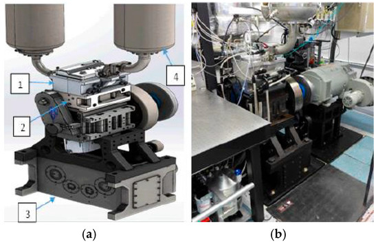
Figure 1.
Experimental diesel engine [26,27]. Note: (a) Numerical illustration of the test bench, (b) actual illustration of the test bench: 1. cast aluminum cylinder head; 2. custom deck adapter facilitates conversion to optimal engine; 3. reconfiguration, belt-driven Lanchester balancing box; 4. control of intake flow rate, composition, and temper.
This study utilized the characteristics of a 4-stroke, single-cylinder diesel engine equipped with a common rail injection system [28], adapted for dual-fuel operation. Table 1 and Table 2 provide the engine’s technical specifications and the properties of the fuels used.

Table 1.
Technical specification of the engine.
Table 2.
Properties of diesel and methanol [29,30].
2.2. CFD Simulation Framework
Computational fluid dynamics (CFD) simulation is a powerful tool that helps reduce the number of experiments needed to develop a new method. It is particularly suitable for internal combustion engines, where laboratory testing can be expensive. Indeed, in this field, where tests can be costly and time-consuming, computer simulations offer a relevant alternative. Although 0-D models are easy to implement, their performance does not compare to that of CFD models, which rely on numerical calculations in the field of fluid mechanics. This approach requires solving the fundamental fluid mechanics equations within a given geometry, which can, if necessary, be coupled with relevant heat transfer or chemical reaction equations. The use of cost-effective numerical CFD, compared to experimental testing, enables a multiplication of tests. This often constitutes a preliminary step in the development of new techniques related to engine operation or the use of new fuels, which pose many physical challenges requiring appropriate modeling. The code and the implemented calculation algorithm are illustrated in Figure 2 below.
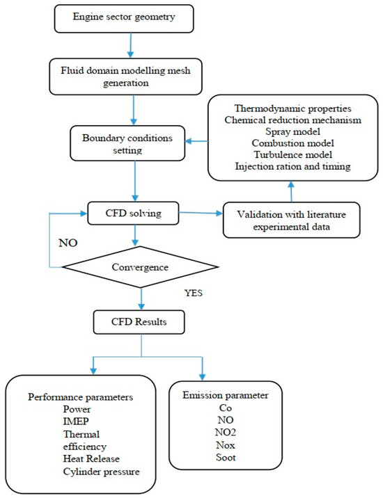
Figure 2.
Diagram of the numerical study.
2.2.1. Geometry and Mesh
Figure 3 provides a three-dimensional illustration of the engine geometry, focusing on the representation of the combustion chamber. To reduce computational time while maintaining model accuracy, a sectorial geometry was chosen. This approach involves modeling only an angular section of the cylinder (typically 45° or 60°, depending on the symmetry of the injector and valves), assuming a symmetric distribution of injection and combustion processes [31].
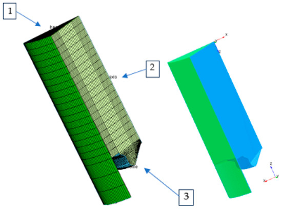
Figure 3.
Geometry and mesh of the cylindrical sector. Note: (1) The cylinder head houses the combustion chamber, valves, and injector, ensuring resistance to high pressures and effective cooling, (2) The liner provides the piston’s sliding surface, ensures sealing, and dissipates heat, (3) The bowl profile determines turbulence and the homogeneity of the air/fuel mixture, directly influencing combustion and emissions.
The computational model incorporates the fundamental components of the combustion chamber, including the piston, cylinder head, valves, and centrally located injector, as well as the cylinder volume, which varies according to the piston displacement. This configuration provides a robust framework for accurately capturing the complex physical and chemical processes governing mixture preparation, fuel atomization, combustion dynamics, and pollutant formation in Diesel engines [32].
We refine the mesh distribution in the injection zone and within the combustion chamber to ensure higher resolution of pressure and temperature gradients, as well as multiphase interactions between the atomized fuel and the intake air. This sectorial model serves as the foundation for the CFD simulation of combustion and emission in the context of our research.
2.2.2. Governing Equations of CFD
Eulerian Phase
The Eulerian phase includes the gaseous phase of the fuel as well as the surrounding air. The Navier–Stokes equations, focused on the conservation of mass, momentum, and energy, are used to represent the behavior of this phase [33,34]. We use Equation (1) to ensure mass conservation:
With the vapor density , the components of the Eulerian velocity , and the source term arising from droplet evaporation, this term ensures the coupling between the Lagrangian and Eulerian phases. The source term accounts for the mass transferred to the Eulerian phase due to the evaporation of the liquid phase.
For the conservation of momentum, Equation (2) is used.
with the absolute pressure p and the stress tensor given by Equation (3):
with the Kronecker delta symbol . The source term arises from the drag force exerted by the droplets and corresponds to the momentum transfer in the opposite direction.
For energy conservation, Equation (4) is used:
For energy conservation, Equation (4) is used: and heat flux are calculated with Equations (5) and (6).
with adiabatic index of gas and thermal conductivity index gas. The term heat transfer source is the inverse of heat change caused by evaporation and conduction.
Lagrangian Phase
The Lagrangian phase contains the liquid phase of the fuel. This phase is superimposed on the Eulerian phase, and transfer terms make it possible to link the two phases. The equation to be solved is that of conservation of momentum.
The momentum contains the forces that are applied to the drop, namely drag force FT, virtual mass FMV and gravity g. The equations for the forces FT and FMV are given by Equations (8) and (9).
Relative Reynolds numbers and drag coefficient are calculated with Equations (10) and (11).
The term drag is the dominant term in the equation, considering the high relative velocity of droplets in ambient air. The virtual mass force is calculated with the inertia of the displaced volume and is proportional to the density of the fluid. Since air is much less dense than fuel, this term is quite weak, and it is possible to overlook it. Since the size of the drops is less than 0.1 mm, the force of gravity is minimal, which also makes it possible to neglect the term gravity. By limiting the equation of the balance of forces to the drag forces, it is possible to write the equation of conservation of momentum as follows:
2.2.3. Combustion Modeling
Turbulence Models (Standard k-ε and RNG k-ε)
Turbulence modeling is essential for simulating reactive flows. In this study, two turbulence models were used: the conventional k-ε model and the RNG k-ε model.
The standard k-ε model is based on two separate transport equations: the first addresses turbulence related to kinetic energy (k), while the second concerns the dissipation rate (ε). Although this model is robust and has been successfully implemented in industrial simulations, it may face limitations in regions with strong shear or significant velocity gradients. The RNG k-ε model is an evolution of the standard k-ε model, developed through the application of the Renormalization Group (RNG) technique. This model provides increased accuracy in highly swirling flows, turbulent jets, and recirculation zones, making it particularly suitable for combustion scenarios in dual-fuel engines [31].
Modèle Standard k-ε
Developed by Launder and Spalding, this model is the simplest of the turbulence models commonly used in CFD. The k-ε model is a semi-empirical model that assumes the flow is fully turbulent and that the effects of molecular viscosity are negligible. It uses two transport equations to independently determine the turbulent kinetic energy k and its dissipation rate ε [35]. The model is numerically efficient, robust, and sufficiently accurate for many turbulent flow applications. It is generally popular in industrial contexts. The transport equations of k and ε are written according to Equations (13) and (14).
In these equations, , , , , are model constants. The source terms involved are calculated based on the probability distribution function of the droplets. Physically, represents the negative rate at which turbulent eddies perform dispersion work on the spray droplets. A value of Cs =5 has been suggested, based on the assumption of length scale conservation during interactions between the jet and the turbulence.
Modèle RNG k-ε
This model is a modified version of the standard k-ε model. In the RNG model, the k equation is exactly the same as in the standard model. However, the mathematical derivation of the ε equation is more rigorous and does not rely on empirically derived constants [36,37].
where the last term RRR on the right-hand side of the equation is defined as follows:
with
and is the mean strain rate tensor.
Compared to the standard ε equation, the RNG model includes an additional term that accounts for anisotropic turbulence [33].
The values of the model constants Prk, Prꜫ, , , used in the RNG version are also listed in Table 3. In the ANSYS Forte 19.0 implementation, the RNG variable value is based on the work of Ji et al. [34], who modified the constant to account for compressibility effects.
where , for an ideal gas, and…
with
Table 3.
Values of the constants in the standard k-ε and RNG k-ε turbulence models.
Using this approach, the value of Cꜫ3 varies within a range from to , and in ANSYS Forte, it is determined automatically based on the flow conditions and the specification of the other model constants and β; Ref. [38] applied their version of the RNG k-ε model to engine simulations and observed improved results compared to the standard model.
2.2.4. KH-RT Injection Model
To enhance combustion modeling, two additional aspects are examined to achieve a more accurate representation of the air–fuel mixture and injection processes. First, a sensitivity analysis on the spray–spray interaction threshold is conducted to assess the impact of fuel jet interactions within a flexible injection strategy [39]. This study helps identify the precise moment when the fuel jets begin to interact significantly, thereby influencing the composition and homogeneity of the air–fuel mixture. Adjusting this parameter is essential to ensure optimal control of the initial combustion conditions.
The Kelvin–Helmholtz Rayleigh–Taylor (KH-RT) model describes spray atomization. It considers instabilities arising from Kelvin–Helmholtz (KH) waves due to aerodynamic forces and Rayleigh–Taylor (RT) instabilities due to body forces. Reitz established correlations for the wavelength () and growth rate (Ω) of the fastest-growing KH instabilities [40].
where is the initial droplet radius, Z is the Ohnessorge number, is the Taylor number, and is the Weber number based on gas properties (note: original Equations (8) and (9) reformatted for clarity).
Turbulent Flame Propagation Model (G-Equation)
The G-equation model, based on Peters’ flamelet concept for premixed turbulent combustion, describes the propagation of the flame front. It is applicable to both wrinkled flamelet and thin reaction zone regimes. The model, as formulated by Wang et al. [41] and Liang et al. [42] for internal combustion engines, uses Favre-averaged equations for the G-field and its variance . In addition, a model equation is used for the ratio between the surface of a turbulent and laminar flame . Using the equation for the surface ratio between the turbulent flame and the laminar flame, we obtain a precise expression for the velocity of the turbulent flame . The complete set of equations to describe the propagation of the premixed turbulent flame front is formed using the mean Navier–Stokes equations on Reynolds and the turbulence modeling equations. The equations used in ANSYS Forte are as follows:
where denotes the tangential gradient operator; is the velocity of the fluid; vertex is the velocity of the moving vertex; and are the average densities of the unburned and burnt mixtures, respectively; is turbulent diffusivity; is the average curvature of Favre’s flame front; , , , et are modeling constants; et are the average Favre turbulent kinetic energy and its dissipation rate from the RNG model k-ε (note: original Equations (10) and (11) adapted for more standard G-equation representation).
NOx Model
Primarily, combustion causes the production of nitrogen oxides (NOx) at high temperatures. It results from chemical reactions between the nitrogen contained in the air and oxygen, mainly through the thermal Zeldovich mechanism. This process involves the gradual formation of nitric oxide (NO) via reversible reactions that depend on temperature, oxygen and nitrogen levels, as well as the residence time in the combustion zone. Through oxidation, NO can then be converted into nitrogen dioxide (NO2). Many researchers have looked at the process of NO formation. Nevertheless, Yakhot et al. [43] highlighted the function of the following reactions in the formation of NO. The concentration of NO is determined by distinguishing the combustion process, i.e., by a post-processing method based on the reversible reactions of the Zeldovich mechanism:
where, the following notations have been introduced, designating by the equilibrium concentrations. The concentration of NO in Equation (27) can be converted into a mass fraction as:
where R1, R2, R3 are reaction rates, is equilibrium concentration, is molar mass of NO, is density.
Soot Model
Soot formation is a complex phenomenon that occurs especially during incomplete combustion, particularly when the fuel is rich. It is common in diesel engines and those operating with dual fuels. Soot consists of carbon particles that form, grow, agglomerate, and can subsequently be oxidized in the combustion chamber. An empirical two-step model is often used, accounting for soot formation and oxidation. The Kadota and Hiroyasu model (1983) is frequently employed for engine simulations [44]. The net rate of soot mass change is:
where is the net soot mass formed, is fuel vaporized mass, is oxygen mole fraction, and are activation energies for formation and oxidation, P is pressure, T is temperature, and are parameters that can be adjusted to match the simulation to the experiment.
2.2.5. Boundary and Initial Conditions
Appropriate boundary and initial conditions are crucial for accurate CFD simulations. Table 4 lists the conditions used.
Table 4.
Initial and boundary conditions for CFD simulation [45].
2.2.6. CFD Model Validation
The simulation results from our previous study are considered. Nang et al. [45] analyzed the combined effects of spray tilt angle, methanol concentration, and turbulence model on the combustion efficiency and pollutant emissions of a diesel engine operating in dual-fuel mode. Several configurations were examined, combining different spray angles (60° and 63°), methanol concentrations (12% and 50%), as well as two turbulence models (standard k-epsilon and RNG k-epsilon).
The optimal configuration identified, namely 25% methanol, a spray angle of 63°, and the RNG k-ε turbulence model, was selected for the validation and exploitation of CFD results in the present study. The numerical data obtained from this configuration were compared with experimental measurements of in-cylinder pressure and heat release rate (HRR) provided by Sandia National Laboratories.
Figure 4 shows the simulated pressure and heat release curves obtained using the CFD model, while Figure 5 compares these numerical results with the corresponding experimental data. Remarkable agreement is observed between the experimental and simulated profiles, particularly during the pressure rise phase and at the peak of heat release.
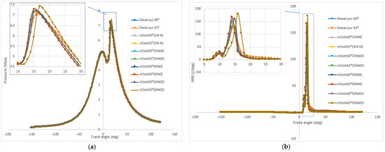
Figure 4.
Simulated curves of in-cylinder pressure and heat release rate. Note: (a) Heat release rate variation and (b) Cylinder pressure variation.
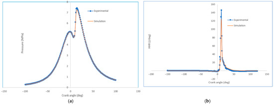
Figure 5.
CFD model validation: comparison of simulated in-cylinder pressure and heat release rate for the CH3OH 63° 25% RNG k-ε configuration with experimental data. Note: (a) Validation of cylinder pressure and (b) Validation of heat release rate.
The deviation at the simulated peak pressure is less than 15%, and the heat release profile closely follows the trend of the experimental data [46]. These findings confirm that the current CFD model configuration accurately and reliably reproduces the thermodynamic behavior of the engine, providing a solid foundation for generating the data used to train our predictive model.
3. Dataset and Preprocessing
The dataset used for developing and validating regression models must accurately reflect the engine mechanisms, providing sufficient detail to capture the fluctuations in combustion parameters and harmful emissions in a dual-fuel engine. This study is based on a dataset obtained from simulations conducted at an engine speed of 2000 rpm, using the RNG k-ε turbulence model, with a spray angle set at 63° and a methanol proportion of 25%. These parameters were selected due to the low discrepancy observed between experimental and simulated data regarding cylinder pressure. The simulation experiment was conducted in transient mode, with fine angular resolution (0.2°), aiming to capture transient events throughout the engine cycle. The adjustment of engine parameters is performed for each specific crankshaft position. Each angular phase includes numerous parameters, such as cylinder pressure, temperature, and local pollutant concentrations (NOx, soot, among others). This method allows for monitoring the progression of parameters throughout the entire engine cycle, from intake (−151°) to exhaust (121°). For each crankshaft angle, the parameters are then extracted and stored. The entire database comprises 1370 cases covering 32 combustion and pollutant emission parameters.
3.1. Choice of Input and Output Variables
In engine modeling, parameters related to combustion and pollutant emissions are crucial, particularly for dual-fuel engines. This research focused on pressure, temperature, NOx, and soot emissions due to their direct impact on energy efficiency, overall performance, and pollutant contributions [47]. These parameters aid in understanding combustion mechanisms and optimizing engine operation for environmental compliance and performance. Table 5 presents the selected parameters.
Table 5.
Combustion and emissions parameters.
3.2. Dataset Partitioning
The dataset was divided into two parts: one for training and the other for testing. The regression model was trained on the training data to identify underlying patterns, while the validation samples were used to evaluate the performance of the selected model. The training dataset can also be split into separate groups for training and validation, with the latter used to fine-tune the algorithmic model. When enough data are available, the “hold-out” technique [48] is applied to divide the dataset as follows: 70% for training and 30% for testing. However, this technique can lead to overfitting of the regressor, especially when the dataset is insufficient in size. In this context, cross-validation techniques such as sequential K-fold (or temporal K-fold) can be applied. In this technique, the dataset is regularly divided into K parts (or folds). Unlike traditional K-fold, this approach is specifically designed for time-series data, where preserving the data sequence is crucial. It involves segmenting the dataset into K successive subsets while maintaining the chronological order of the observed data.
The sequential K-fold technique involves progressively using an increasing number of folds for training, while the next fold is used for evaluation. For example, in the first iteration, the model is trained on the first data batch and tested on the second. In the next iteration, the first two segments are used for training, while the third is used for testing, and this process repeats. This continues until each segment has been used at least once as a test set, without ever introducing future data into the training process [49,50]. In this study, particular attention was given to the choice of the parameter K in sequential K-fold cross-validation, considering the temporal dimension and the data volume. The selection of K is important, as it directly influences the relevance of the model evaluation, the processing time required, and the risk of overfitting. In theory, a higher K value (such as K = 8 or 10) provides a more accurate assessment since the model is tested on a wider range of segments and benefits from multiple trainings on different partitions.
However, this alternative significantly increases the computational load, which can be problematic for complex models, especially those using neural networks [51]. Furthermore, in the context of time series, an excessively high K selection could lead to smaller, less representative, and noisier test samples, thereby reducing the reliability of the evaluation. Conversely, a too-low K (such as K = 2 or 3) generates larger test sets while decreasing the number of iterations during cross-validation. This could reduce the statistical robustness of the results and provide a less accurate representation of the model’s generalization capability. Thus, the selection of the optimal K is based on a balance between the representativeness of the data analyzed, the amount of information available for training, and the intended generalization. For a dataset of intermediate size, K values ranging between 4 and 6 are often considered appropriate. This study uses four K-fold segments, as illustrated in Figure 6.
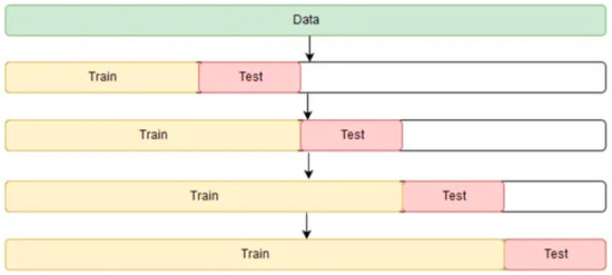
Figure 6.
Sequential K-fold cross-validation blocks [50].
3.3. Normalization
Normalization (or standardization) is an initial data processing step to scale features and reduce model complexity, often required by certain algorithms. Standardizing data to have zero mean and unit variance can improve learning by eliminating discrepancies arising from different scales and distributions [52]. The transformation is as follows:
where is the normalized data, is the original feature vector, m is the mean of the mean of the feature, and σ is its standard deviation.
3.4. Description of the GRU Model
For time-series predictive analysis, recurrent neural networks (RNNs) and their variants are frequently employed. Compared to traditional neural networks, RNNs possess a unique memory structure that allows them to associate the influence of past data with the current learning and training process, leading to more optimal predictions [53]. However, since only a single tanh unit is used, issues such as vanishing or exploding gradients often arise during the training process. In response to this issue, the Long Short-Term Memory (LSTM) network and the Gated Recurrent Unit (GRU) were developed as improvements over the standard RNN. These architectures are specifically designed to overcome the vanishing gradient problem and enhance the model’s prediction performance.
The LSTM is essentially composed of a forget gate, an input gate, and an output gate. The main function of the forget gate is to discard irrelevant or invalid information. The input gate selects incoming data by retaining only the most relevant information. The output gate is responsible for passing useful information to the next layer [54]. LSTM enhances the traditional RNN by modifying the internal structure of the neurons and addressing the vanishing gradient problem. However, due to its more complex internal structure, the model incorporates a greater number of activation functions and learnable parameters, which makes training more challenging and slows down prediction speed.
To improve the prediction speed of the model while ensuring prediction accuracy, it is necessary to simplify the model’s internal structure as much as possible, making it easier to understand and implement. Therefore, some researchers have proposed the Gated Recurrent Unit (GRU) network.
The GRU is also considered an activator in the context of recurrent neural networks, proposed as a response to challenges such as long-term memory and gradient issues during backpropagation [55]. The GRU shares similarities with the LSTM. By optimizing the internal structure of the LSTM network, an update gate is used to replace the functions of the input and forget gates within the network. Consequently, compared to the LSTM, the GRU has a reduced number of parameters [56]. In the GRU, the reset gate is used to merge information from the previous state with that of the current state to obtain the output for the present state. The update gate retains only the previous hidden state by retrieving the previous hidden state , the current input , and the current state information . It then applies a nonlinear transformation using the activation function to the combined matrix. In other words, this means ignoring some minor information in and selectively retrieving certain data in . The basic structure of the GRU is illustrated in Figure 7, and the corresponding mathematical formulas are presented in Equation (31).
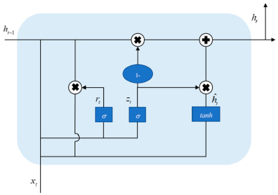
Figure 7.
Structure of the GRU cell [56].
In the formula, , , , , and , respectively, represent the current-time input information, the previous time-time hidden state, the update gate, the reset gate, the candidate hidden state, and the now-time hidden layer output. , , are the matrix of the weight parameters of the GRU neural network. σ is the sigmoid function.
3.5. Regression Metrics
The purpose of model evaluation is to assess its accuracy and efficiency. First, it is essential to examine a model’s generalization ability in order to compare various models and determine whether one outperforms the others. These indicators subsequently help to gradually improve the performance of our models. This study selects four commonly used evaluation metrics in deep learning: Mean Squared Error (MSE), Root Mean Squared Error (RMSE), Mean Absolute Error (MAE), and the Pearson Product-Moment Correlation Coefficient [57,58]. The corresponding equations are presented in Equation (32).
In the formula, represents the predicted value and the actual (real) value.
The MSE evaluates the discrepancy between the estimated value and the actual value. The Root Mean Squared Error (RMSE) is defined as the square root of the ratio between the sum of the squared errors—derived from the predicted and actual values—and the number of observations n. The Mean Absolute Error (MAE) is defined as the average of the absolute differences between each predicted value and the actual value. Using the MAE eliminates the issue of errors canceling each other out, enabling a more accurate assessment of the actual magnitude of the prediction error. The Mean Absolute Percentage Error (MAPE) reflects the average error as a percentage of the actual values, thereby allowing for easy comparison across datasets with different scales. Regarding the Pearson correlation coefficient, it is frequently used as a statistical measure of accuracy, as it facilitates the assessment of the strength and direction of the linear relationship between observed and predicted values. A result close to 1 indicates a strong positive correlation, highlighting the effectiveness of the predictive model. Finally, the Kling–Gupta Efficiency (KGE) is a metric that combines three components: bias, correlation, and variability between the predicted and observed series. It provides a more comprehensive evaluation of prediction quality than a single indicator. A KGE value close to 1 demonstrates strong model performance in terms of accuracy, temporal structure, and variability.
3.6. Feature Vector
The input (feature) vector for the GRU model consists of a sequence of parameters (pressure, temperature, NOx, soot) evaluated at specific crankshaft angle steps. Equation (33) represents this organized matrix, capturing engine dynamics over an interval θL (sequence length):
- : Pressure at angle step ;
- : Temperature at angle step ;
- : Emissions at angle step ;
- : Soot emissions at angle step.
Each row of this vector represents a set of combustion and emission parameters for a given angle , spanning over . The output vector is a prediction for the next crankshaft angle, , and has the following form:
- : Pressure at angle step ;
- : Temperature at angle step ;
- : NOx emissions at angle step ;
- : Soot emissions at angle step .
4. Results and Discussion
The regression analysis of combustion parameters and pollutant emissions followed a procedure similar to that adopted by Paul et al. [59] and Ji et al. [60], evaluating the system’s ability to model the engine combustion process.
4.1. Hyperparameter Tuning of the Regressor
Hyperparameter tuning is a crucial step in establishing an effective prediction model. This phase involves adjusting parameters external to the model, such as the size of the layers, the number of iterations, or the degree of regularization. These factors have a direct impact on learning efficiency and the model’s ability to generalize to previously unseen data. In this research, hyperparameter tuning of the GRU model was carried out using Keras Tuner, an automated tool specifically designed to efficiently search for optimal configurations. Keras Tuner offers various search strategies, such as Random Search, the Hyperband technique, and Bayesian optimization [61]. These methods help reduce the number of required trials while focusing on promising regions within the hyperparameter space. In this research, Random Search was preferred due to its ease of use, fast execution, and ability to efficiently explore the search space without requiring prior modeling of the model’s behavior. Instead of performing an exhaustive search (Grid Search), Random Search allows for exploration of a wide range of combinations while keeping computational cost moderate, which is particularly beneficial when optimizing a large number of parameters. Although this method is not as sophisticated as other strategies such as Bayesian optimization, it has proven useful in identifying effective hyperparameter combinations within a reasonable timeframe. The configured hyperparameters include the number of neurons in the GRU hidden layer, the batch size, the number of epochs, and the dropout rate applied to prevent overfitting.
For each combination analyzed, sequential cross-validation using K = 4 folds was applied. This approach preserves the chronological order of the data, ensuring a robust evaluation that respects their temporal nature. The selected performance metric is the mean of the Mean Squared Error (MSE) calculated across the different folds, allowing for the identification of the most effective hyperparameter configurations (Figure 8), Table 6 clearly illustrates the hyperparameters selected for the model training. This automated optimization method, combined with time-series-specific cross-validation, ensures that the selected GRU model has a strong generalization ability while efficiently managing the required computational resources.
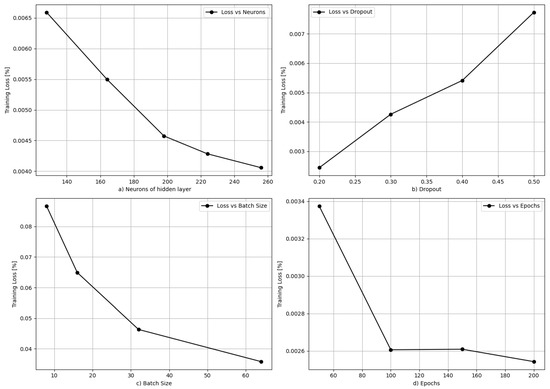
Figure 8.
Evolution of training and test loss functions with epoch number for the GRU model.
Table 6.
Optimized GRU hyperparameters.
Figure 9 shows the evolution of training and testing loss for the GRU model over 200 epochs after hyperparameter tuning. A sharp reduction in loss occurs within the first ~20 epochs, indicating rapid initial learning. Subsequently, training and test loss curves converge to low, stable levels, suggesting effective generalization without significant overfitting. The small gap between training and test losses indicates that the model predicts unseen data with accuracy comparable to its performance on training data, implying an appropriate fit.
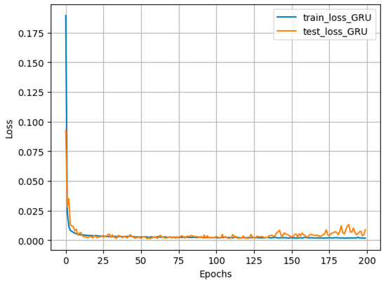
Figure 9.
Evolution of training and test loss functions with epoch number for the GRU model.
4.2. Regression Testing and Validation with Experimental Data
Predicted results from the proposed GRU model were compared with the experimental (CFD-derived baseline) results for cylinder pressure, temperature, NOx, and soot emissions, as shown in Figure 10, Figure 11, Figure 12 and Figure 13 (assuming these figures are available and correctly show experimental vs. predicted plots, scatter plots, and error metrics). The overall correlation coefficient (R) of 0.9975 indicates a high degree of correlation between the GRU model’s predictions and the target values. This implies that 99.75% of the variations in the experimental (CFD) results are explained by the GRU model’s predictions. The GRU model achieved a training loss (MSE) of 0.0013. Cross-validation results indicated good agreement between training and validation loss, confirming the model’s generalization capability.
4.2.1. Cylinder Pressure
Figure 10a–c (assumed content) display the correlation, time-series comparison, and error distribution for cylinder pressure prediction. Figure 10b (assumed) shows a comparison between the experimentally measured (CFD baseline) pressure and the GRU-predicted pressure over the analyzed crank angle range. For pressure prediction, an RMSE of 0.0117, MSE of 0.00013, and MAE of 0.01 were observed (from Figure 14 text), resulting in a MAPE of 0.081%, which is considered highly satisfactory. The prediction error is less than 1% (based on MAPE), indicating the model’s ability to accurately capture combustion dynamics, even with methanol presence. Correlation metrics (from Figure 15 text) were R = 0.9998, R2 = 0.9993, and KGE = 0.9775. These values suggest the model accurately reproduces test conditions and generalizes effectively. The GRU model’s capability to predict pressure values associated with complex combustion processes reflects efficient modeling of methanol’s influence and turbulence effects.

Figure 10.
Comparison of GRU-predicted cylinder pressure (P) with experimentally measured (CFD baseline) pressure: (a) scatter plot, (b) time-series overlay, (c) error analysis.
4.2.2. Cylinder Temperature
Figure 11a–c (assumed content) compare GRU-predicted temperature with empirically estimated (CFD baseline) temperature. The ch3oh-63°-25–RNGk-ε mixture was noted as achieving the optimal temperature among those tested in the CFD simulations. Figure 11b (assumed) compares experimental (CFD baseline) temperature with model estimates versus crank angle. For temperature, RMSE, MSE, and MAE values were 0.0179, 0.0003, and 0.0111, respectively (from Figure 14 text), with a MAPE of 0.013%. Correlation metrics (from Figure 15 text) were R = 0.9989, R2 = 0.9976, and KGE = 0.9929. Minor discrepancies observed around 80° crank angle might be attributable to complex turbulent interactions during combustion, as modeled by RNG k-ε, not fully captured by the GRU or indicating areas for hyperparameter refinement.

Figure 11.
Comparison of GRU-predicted temperature (T) with experimentally measured (CFD baseline) temperature: (a) scatter plot, (b) time-series overlay, (c) error analysis.
4.2.3. Nitrogen Oxide (Nox) Emissions
Figure 12a–c (assumed content) illustrate the relationship between GRU-predicted NOx and experimentally measured (CFD baseline) NOx. The CFD simulations indicated that incorporating methanol tended to reduce NOx emissions, with the ch3oh-63°-25–RNGk-ε configuration showing a significant reduction. For NOx emission prediction, the GRU model achieved an RMSE of 0.0427, MSE of 0.0018, MAE of 0.0318 (from Figure 14 text), and a MAPE of 0.0286%. Correlation metrics (from Figure 15 text) were R = 0.9974, R2 = 0.9920, and KGE = 0.9474. A slight divergence in the test curve from experimental data around the 80-degree crank angle (Figure 12b, assumed) could stem from variations in combustion conditions or limitations in modeling local factors affecting NOx. Further model refinement or data augmentation could enhance robustness.

Figure 12.
Comparison of GRU-predicted NOx emissions with experimentally measured (CFD baseline) NOx: (a) scatter plot, (b) time-series overlay, (c) error analysis.
4.2.4. Soot Emissions
Figure 13a–c (assumed content) compare GRU-generated soot emissions with experimentally measured (CFD baseline) values. The ch3oh-63°-25%-RNGk-ε CFD simulation showed the lowest soot emissions compared to pure diesel operation. Model predictions closely matched experimental (CFD baseline) results, demonstrating good generalization (Figure 13b, assumed). The correspondence between training/test predictions and target values (Figure 12c, assumed) suggests no significant overfitting. Error metrics for soot (from Figure 14 text) were RMSE = 0.0465, MAE = 0.0278, and MSE = 0.0021, with a MAPE of 0.0249%, considered satisfactory. Correlation metrics (from Figure 15 text) were R = 0.9952, R2 = 0.9882, and KGE = 0.9563. Minor variations are permissible. The GRU model’s ability to capture methanol’s impact on reducing soot emissions highlights its potential for optimizing engine operation for lower pollutant output.

Figure 13.
Comparison of GRU-predicted soot emissions with experimentally measured (CFD baseline) soot: (a) scatter plot, (b) time-series overlay, (c) error analysis.

Figure 14.
Comparison of model error metrics (RMSE, MAE, MSE, MAPE) for pressure, temperature, NOx, and soot on the test set.

Figure 15.
Comparison of model correlation coefficients (R, R2, KGE) for pressure, temperature, NOx, and soot on the test set.
The error analysis (RMSE, MSE, MAE, MAPE) across parameters indicates the model’s consistent performance in predicting combustion and emission characteristics. Slightly higher RMSE and MAE for temperature (T) and NOx, compared to pressure, might be attributed to the greater complexity and sensitivity of these processes. The MSE values were generally low (around 0.0013 overall, as per Abstract/text), signifying that the model predicts parameters without significant dispersion, aligning with acceptable thresholds mentioned by Paul et al. [59] and Najafi et al. [58]. Correlation coefficients (R, R2, KGE) reveal a strong relationship between GRU predictions and target data for all parameters, generally close to 1 by Paul et al. [59]. This ensures the model effectively captures data trends according to Ji et al. [60]. The KGE values, while slightly lower for some parameters than R or R2, are still significant, indicating adequate error distribution. While the RNG k-ε model (used for data generation) showed adequate matching in turbulence simulations, the GRU model’s ability to directly learn from these complex, high-dimensional data enhances its overall predictive power for these transient engine processes. This underscores the advantage of using recurrent neural networks for complex combustion prediction tasks.
4.3. Global Prediction Error Analysis and Parameter Sensitivity
The examination of global prediction errors reveals performance varies depending on the parameters considered. As shown in Figure 16, for the variable pressure, the residuals exhibit a bimodal distribution, suggesting possible model non-conformities or missing explanatory factors. This fluctuation highlights a marked sensitivity of the model to this parameter, while still maintaining average prediction accuracy. In contrast, the temperature variable shows slightly scattered residuals centered around zero, although somewhat asymmetric. This reflects the model’s ability to accurately predict this variable while remaining relatively insensitive to perturbations. Regarding NOx, the residuals display clear asymmetry with extreme negative values, indicating that the model tends to underestimate this variable. This wide dispersion underscores the parameter’s high responsiveness and suggests the need for model refinement or the inclusion of additional explanatory features. Finally, the soot residuals cluster predominantly around zero, demonstrating excellent predictive capability and low sensitivity for this parameter. Overall, the model performs remarkably well in predicting temperature and soot variables.
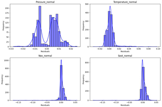
Figure 16.
Residual value distribution map.
4.4. Comparison of Results with Other RNN Models
This work employs a comparative experimental approach to establish the validity and effectiveness of the proposed GRU predictive model, highlighting its high accuracy and reliability in the practical task of parameter forecasting. The GRU prediction model is compared with three other prediction models, namely LSTM, BiLSTM, and BiGRU. Before starting the experimental comparison, it is crucial to ensure that the input data for each model correspond to the same standardized dataset after processing, and that hyperparameter tuning has been accurately performed for each model, taking into account their distinct characteristics. It is also essential to ensure maximum consistency in the input parameters of the models and the experimental conditions during the comparisons, in order to facilitate the evaluation of prediction accuracy, model training speeds, and so on. By assessing the models using various performance metrics, one can accurately highlight the strengths and weaknesses of each model in the context of the actual predictive task. The upcoming figures will provide a visual comparison of the prediction results generated by the different models.
After completing the training, the time required for each model to predict a step in the test process is recorded as shown in Table 7.
Table 7.
Comparison of time required for single step of each model.
Figure 17, Figure 18, Figure 19 and Figure 20 show that the GRU prediction model provides the most accurate fit and the highest degree of similarity to the actual data compared to the other prediction models. According to Figure 21 and Figure 22, the performance index of the GRU model exhibits the lowest error compared to the others, indicating minimal discrepancy between the model’s predicted value and the actual value.
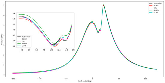
Figure 17.
Comparison of cylinder pressure predictions by different models.
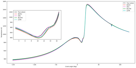
Figure 18.
Comparison of cylinder temperature predictions by different models.
Figure 19.
Comparison of NOx predictions by different models.
Figure 20.
Comparison of soot predictions by different models.
Figure 21.
Summary of evaluation indicators for the prediction results of different models during training.
Figure 22.
Summary of evaluation indicators for the prediction results of different models during testing.
5. Conclusions
This study presented a GRU-based deep learning model for predicting combustion (cylinder pressure, temperature) and pollutant emission parameters (NOx, soot) in a diesel engine operating in dual-fuel mode with methanol. The primary conclusions are as follows:
- -
- Data preprocessing, including normalization, effectively mitigated the impact of varying magnitudes and orders of magnitude across different prediction parameters.
- -
- The proposed GRU model can automatically learn time-series characteristics from the CFD-generated engine data.
- -
- Comparative experiments against LSTM, BiLSTM, and BiGRU models, based on evaluation metrics (RMSE, MAE, MSE), demonstrated that the GRU model achieved higher prediction accuracy for this specific task, highlighting its advantages for time-series prediction of engine parameters.
- -
- The prediction model exhibits acceptable accuracy (e.g., overall MAPE of 0.0251%, R of 0.9975), providing a reliable tool for interpreting engine behavior and potentially identifying deviations indicative of early-stage faults.
- -
- The model’s ability to accurately predict these parameters can facilitate proactive maintenance strategies, potentially reducing downtime and operational costs, thereby playing a crucial role in preventative maintenance and engine health management.
Future work could involve validating the GRU model with experimental data from a physical engine testbed, exploring other advanced deep learning architectures, and expanding the range of predicted parameters or operational conditions.
Author Contributions
Conceptualization, C.V.N.A.; Methodology, J.F.E. and F.P.N.N.; Software, J.F.E.; Validation, F.P.N.N.; Investigation, J.F.E. and F.T.N.; Resources, L.M.A.T.; Data curation, F.P.N.N.; Supervision, C.V.N.A. All authors have read and agreed to the published version of the manuscript.
Funding
This work was funded by the University of Douala and the Ministry of Higher Education of Cameroon.
Institutional Review Board Statement
Not applicable.
Informed Consent Statement
Not applicable.
Data Availability Statement
The raw data supporting the conclusions of this article will be made available by the authors on request.
Acknowledgments
The authors sincerely thank the University of Douala for its support and contribution to the completion of this study.
Conflicts of Interest
The authors declare that they have no conflicts of interest.
References
- Som, S.; Aggarwal, S.K. Effects of primary breakup modeling on spray and combustion characteristics of compression ignition engines. Combust. Flame 2010, 157, 1179–1193. [Google Scholar] [CrossRef]
- Payri, R.; Salvador, F.J.; Gimeno, J.; Peraza, J.E. Experimental study of the injection conditions influence over n-dodecane and diesel sprays with two ECN single-hole nozzles. Part II: Reactive atmosphere. Energy Convers. Manag. 2016, 126, 1157–1167. [Google Scholar] [CrossRef]
- Bardi, M.; Bruneaux, G.; Malbec, L.-M. Study of ECN Injectors’ Behavior Repeatability with Focus on Aging Effect and Soot Fluctuations. In Proceedings of the Présenté à SAE 2016 World Congress and Exhibition, Detroit, MI, USA, 12–14 April 2016. [Google Scholar] [CrossRef]
- Sana, S.S. Optimum buffer stock during preventive maintenance in an imperfect production system. Math. Methods Appl. Sci. 2022, 45, 8928–8939. [Google Scholar] [CrossRef]
- Duan, Y.; Li, Z.; Tao, X.; Li, Q.; Hu, S.; Lu, J. EEG-Based Maritime Object Detection for IoT-Driven Surveillance Systems in Smart Ocean. IEEE Internet Things J. 2020, 7, 9678–9687. [Google Scholar] [CrossRef]
- Liu, J.; Yang, G.; Li, X.; Hao, S.; Guan, Y.; Li, Y. A deep generative model based on CNN-CVAE for wind turbine condition monitoring. Meas. Sci. Technol. 2023, 34, 035902. [Google Scholar] [CrossRef]
- Zhu, Y.; Wu, P.H.J.; Liu, F.; Kanagavelu, R. Disk Failure Prediction for Software-Defined Data Centre (SDDC). In Proceedings of the 2021 IEEE Intl Conf on Dependable, Autonomic and Secure Computing, Intl Conf on Pervasive Intelligence and Computing, Intl Conf on Cloud and Big Data Computing, Intl Conf on Cyber Science and Technology Congress (DASC/PiCom/CBDCom/CyberSciTech), Calgary, AB, Canada, 25–28 October 2021; pp. 264–268. [Google Scholar] [CrossRef]
- Gao, Z.; Jiang, Z.; Zhang, J. Identification of power output of diesel engine by analysis of the vibration signal. Meas. Control. 2019, 52, 1371–1381. [Google Scholar] [CrossRef]
- Shao, S.; McAleer, S.; Yan, R.; Baldi, P. Highly Accurate Machine Fault Diagnosis Using Deep Transfer Learning. IEEE Trans. Ind. Inf. 2019, 15, 2446–2455. [Google Scholar] [CrossRef]
- Han, S.H.; Rahim, T.; Shin, S.Y. Detection of Faults in Solar Panels Using Deep Learning. In Proceedings of the 2021 International Conference on Electronics, Information, and Communication (ICEIC), Jeju, Republic of Korea, 31 January–3 February 2021; pp. 1–4. [Google Scholar] [CrossRef]
- Jana, B.B.; Farmanb, H.; Khanc, M.; Imranc, M.; Islamc, I.U.; Ahmadd, A.; Ali, S.; Jeone, G. Deep learning in big data Analytics: A comparative study. Comput. Electr. Eng. 2019, 75, 275–287. [Google Scholar] [CrossRef]
- Kumar, A.; Srivastava, A.; Goel, N.; McMaster, J. Exhaust gas temperature data prediction by autoregressive models. In Proceedings of the 2015 IEEE 28th Canadian Conference on Electrical and Computer Engineering (CCECE), Halifax, NS, Canada, 3–6 May 2015; pp. 976–981. [Google Scholar] [CrossRef]
- Ismail, H.M.; Ng, H.K.; Queck, C.W.; Gan, S. Artificial neural networks modelling of engine-out responses for a light-duty diesel engine fuelled with biodiesel blends. Appl. Energy 2012, 92, 769–777. [Google Scholar] [CrossRef]
- Zhao, R.; Yan, R.; Wang, J.; Mao, K. Learning to Monitor Machine Health with Convolutional Bi-Directional LSTM Networks. Sensors 2017, 17, 273. [Google Scholar] [CrossRef] [PubMed]
- Saleem, U.; Khan, M.A.; Khan, M.A. EnerNet: Attention-based Dilated CNN-BiLSTM for State of Health Monitoring of Lithium-Ion Batteries. Energy 2025, 276, 126890. [Google Scholar] [CrossRef]
- Alcan, G.; Yilmaz, E.; Unel, M.; Aran, V.; Yilmaz, M.; Gurel, C.; Koprubasi, K. Estimating Soot Emission in Diesel Engines Using Gated Recurrent Unit Networks. IFAC-PapersOnLine 2019, 52, 544–549. [Google Scholar] [CrossRef]
- Zhang, Y.; Liu, P.; He, X.; Jiang, Y. A prediction method for exhaust gas temperature of marine diesel engine based on LSTM. In Proceedings of the 2020 IEEE 2nd International Conference on Civil Aviation Safety and Information Technology (ICCASIT, Weihai, China, 14–16 October 2020; pp. 49–52. [Google Scholar] [CrossRef]
- Shi, B.; Shi, H.; Wang, H. Performance Prediction of Marine Diesel Engine Based on Long Short-Term Memory Network. J. Phys. Conf. Ser. 2020, 1631, 012135. [Google Scholar] [CrossRef]
- Elmaz, F.; Eyckerman, R.; Casteels, W.; Latré, S.; Hellinckx, P. CNN-LSTM architecture for predictive indoor temperature modeling. Build. Environ. 2021, 206, 108327. [Google Scholar] [CrossRef]
- Kayaalp, K.; Metlek, S.; Ekici, S.; Şöhret, Y. Developing a model for prediction of the combustion performance and emissions of a turboprop engine using the long short-term memory method. Fuel 2021, 302, 121202. [Google Scholar] [CrossRef]
- Liu, B.; Gan, H.; Chen, D.; Shu, Z. Research on Fault Early Warning of Marine Diesel Engine Based on CNN-BiGRU. J. Mar. Sci. Eng. 2022, 11, 56. [Google Scholar] [CrossRef]
- Hu, D.; Wang, H.; Yang, C.; Wang, B.; Duan, B.; Wang, Y. Engine combustion modeling method based on hybrid drive. Heliyon 2023, 9, e21494. [Google Scholar] [CrossRef]
- Shen, Q.; Wang, G.; Wang, Y.; Zeng, B.; Yu, X.; He, S. Prediction Model for Transient NOx Emission of Diesel Engine Based on CNN-LSTM Network. Energies 2023, 16, 5347. [Google Scholar] [CrossRef]
- Liu, Y.; Gan, H.; Cong, Y.; Hu, G. Research on fault prediction of marine diesel engine based on attention-LSTM. Proc. Inst. Mech. Eng. Part M: J. Eng. Marit. Environ. 2023, 237, 508–519. [Google Scholar] [CrossRef]
- Pastor, J.V.; García, A.; Micó, C.; Lewiski, F.; Vassallo, A.; Pesce, F.C. Effect of a novel piston geometry on the combustion process of a light-duty compression ignition engine: An optical analysis. Energy 2021, 221, 119764. [Google Scholar] [CrossRef]
- Kosaka, H.; Wakisaka, Y.; Nomura, Y.; Hotta, Y.; Koike, M.; Nakakita, K. Concept of “Temperature Swing Heat Insulation” in Combustion Chamber Walls, and Appropriate Thermo-Physical Properties for Heat Insulation Coat. SAE Int. J. Engines 2013, 6, 142–149. [Google Scholar] [CrossRef]
- Nkol, F.P.N.; Banta, N.J.I.; Offole, F.; Abbe, C.V.N.; Mouangue, R. Effect of direct water injection on emission of pollutants in a diesel engine using CFD and water/fuel mass ratio based parametric analysis. arXiv 2022. [Google Scholar] [CrossRef]
- Teoh, Y.H.; Tan, S.S.; Tan, S.S.; Tan, C.S. Implementation of Common Rail Direct Injection System and Optimization of Fuel Injector Parameters in an Experimental Single-Cylinder Diesel Engine. Int. J. Mol. Sci. 2020, 21, 2099. [Google Scholar] [CrossRef]
- Yao, C.; Cheung, C.S.; Cheng, C.; Wang, Y.; Chan, T.L.; Lee, S.C. Effect of Diesel/methanol compound combustion on Diesel engine combustion and emissions. Energy Convers. Manag. 2008, 49, 1696–1704. [Google Scholar] [CrossRef]
- Cheng, C.H.; Cheung, C.S.; Chan, T.L.; Lee, S.C.; Yao, C.D. Experimental investigation on the performance, gaseous and particulate emissions of a methanol fumigated diesel engine. Sci. Total Environ. 2008, 389, 115–124. [Google Scholar] [CrossRef]
- Perini, F.; Busch, S.; Kurtz, E.; Warey, A.; Peterson, R.C.; Reitz, R. Limitations of Sector Mesh Geometry and Initial Conditions to Model Flow and Mixture Formation in Direct-Injection Diesel Engines. In Proceedings of the Présenté à WCX SAE World Congress Experience, Detroit, MI, USA, 2 April 2019; p. 2019-01-0204. [Google Scholar] [CrossRef]
- Totla, N.B.; Bhalerao, Y.J. CFD simulation of in cylinder combustion of multi-cylinder diesel engine. Mater. Today Proc. 2024, 102, 31–51. [Google Scholar] [CrossRef]
- Zawawi, M.; Saleha, A.; Hassan, N.H. A review: Fundamentals of computational fluid dynamics (CFD). In Proceedings of the Présenté à Green Design and Manufacture: Advanced and Emerging Applications: Proceedings of the 4th International Conference on Green Design and Manufacture 2018, Ho Chi Minh, Vietnam, 29–30 April 2018; p. 020252. [Google Scholar] [CrossRef]
- Ji, G.; Zhang, M.; Lu, Y.; Dong, J. The Basic Theory of CFD Governing Equations and the Numerical Solution Methods for Reactive Flows. In Computational Fluid Dynamics—Recent Advances, New Perspectives and Applications; Ji, G., Dong, J., Eds.; IntechOpen: London, UK, 2023. [Google Scholar] [CrossRef]
- Smith, L.M.; Reynolds, W.C. On the Yakhot–Orszag renormalization group method for deriving turbulence statistics and models. Phys. Fluids A Fluid Dyn. 1992, 4, 364–390. [Google Scholar] [CrossRef]
- Han, Z.; Reitz, R.D. Turbulence Modeling of Internal Combustion Engines Using RNG κ-ε Models. Combust. Sci. Technol. 1995, 106, 267–295. [Google Scholar] [CrossRef]
- Wilcox, D.C. Reassessment of the scale-determining equation for advanced turbulence models. AIAA J. 1988, 26, 1299–1310. [Google Scholar] [CrossRef]
- Launder, B.E.; Spalding, D.B. The numerical computation of turbulent flows. Comput. Methods Appl. Mech. Eng. 1974, 3, 269–289. [Google Scholar] [CrossRef]
- An, C.; Zhou, B.; Liu, Y.; Li, X.; Nishida, K. Threshold sensitivity study on spray–spray impingement under flexible injection strategy for fuel/air mixture evaluation. Phys. Fluids 2025, 37, 065124. [Google Scholar] [CrossRef]
- Fu, J.; Liu, J.; Ma, Y.; Wang, S.; Deng, B.; Zeng, D. Effects of injector spray angle on combustion and emissions characteristics of a natural gas (NG)-diesel dual fuel engine based on CFD coupled with reduced chemical kinetic model. Appl. Energy 2019, 233–234, 182–195. [Google Scholar] [CrossRef]
- Wang, B.-L.; Bergin, M.J.; Petersen, B.R.; Miles, P.C.; Reitz, R.D.; Han, Z. Validation of the Generalized RNG Turbulence Model and Its Application to Flow in a HSDI Diesel Engine. In Proceedings of the Présenté à SAE 2012 World Congress & Exhibition, Detroit, MI, USA, 2 April 2012. [Google Scholar] [CrossRef]
- Liang, L.; Reitz, R.D. Spark Ignition Engine Combustion Modeling Using a Level Set Method with Detailed Chemistry. In Proceedings of the Présenté à SAE 2006 World Congress & Exhibition, Detroit, MI, USA, 3–6 April 2006. [Google Scholar] [CrossRef]
- Yakhot, V.; Orszag, S.A.; Thangam, S.; Gatski, T.B.; Speziale, C.G. Development of turbulence models for shear flows by a double expansion technique. Phys. Fluids A: Fluid Dyn. 1992, 4, 1510–1520. [Google Scholar] [CrossRef]
- Kadota, T.; Hiroyasu, H. Soot concentration measurement in a fuel droplet flame via laser light scattering. Combust. Flame 1984, 55, 195–201. [Google Scholar] [CrossRef]
- Nkol, F.P.N.; Freidy, E.J.; Banta, N.J.I.; Yotchou, G.V.T.; Abbe, C.V.N.; Mouangue, R.M. Simulating the Effect of Methanol and Spray Tilt Angle on Pollutant Emission of a Diesel Engine Using Different Turbulence Models. Int. J. Heat Technol. 2023, 41, 105–1120. [Google Scholar] [CrossRef]
- Bush, S. Sandia’s New Medium-Duty Diesel Research Engine and What We’re Going to Do with It; Sandia National Laboratories: Livermore, CA, USA, 2020. Available online: https://www.osti.gov/servlets/purl/1764673 (accessed on 2 April 2020).
- Duysinx, P. Internal Combustion Engines. Part 1: Principles of Operation and Technologies; University of Liège: Liège, Belgium, 2018–2019; Available online: http://www.ingveh.ulg.ac.be/uploads/education/GCIV-2025/MCGTA6_ICE_PartA_2019.pdf (accessed on 27 August 2025).
- Yadav, S.; Shukla, S. Analysis of k-Fold Cross-Validation over Hold-Out Validation on Colossal Datasets for Quality Classification. In Proceedings of the 2016 IEEE 6th International Conference on Advanced Computing (IACC), Bhimavaram, India, 27–28 February 2016; pp. 78–83. [Google Scholar] [CrossRef]
- Bramer, M. Principles of Data Mining. In Undergraduate Topics in Computer Science; Springer: London, UK, 2016. [Google Scholar] [CrossRef]
- Karouche, I. La Détection des Ruptures et D’anomalies dans les Séries Temporelles. Master’s Thesis, École Nationale Supérieure d’Informatique, Alger, Oued Smar, Algerien, 2020. [Google Scholar] [CrossRef]
- Hestness, J.; Ardalani, N.; Diamos, G. Beyond Human-Level Accuracy: Computational Challenges in Deep Learning. In Proceedings of the 24th Symposium on Principles and Practice of Parallel Programming, Washington DC, USA, 16–20 February 2019; pp. 1–14. [Google Scholar] [CrossRef]
- Sefara, T.J. The Effects of Normalisation Methods on Speech Emotion Recognition. In Proceedings of the 2019 International Multidisciplinary Information Technology and Engineering Conference (IMITEC), Vanderbijlpark, South Africa, 21–22 November 2019; pp. 1–8. [Google Scholar] [CrossRef]
- Mishra, A.; Tripathi, K.; Gupta, L.; Singh, K.P. Long Short-Term Memory Recurrent Neural Network Architectures for Melody Generation. In Soft Computing for Problem Solving; Bansal, J.C., Das, K.N., Nagar, A., Deep, K., Ojha, A.K., Eds.; In Advances in Intelligent Systems and Computing; Springer: Singapore, 2019; Volume 817, pp. 41–55. [Google Scholar] [CrossRef]
- Li, Q.; Wang, B.; Jin, J.; Wang, X. Comparison of CNN-Uni-LSTM and CNN-Bi-LSTM based on single-channel EEG for sleep staging. In Proceedings of the 2020 5th International Conference on Intelligent Informatics and Biomedical Sciences (ICIIBMS), Okinawa, Japan, 18–20 November 2020; pp. 76–80. [Google Scholar] [CrossRef]
- Yu, J.; Zhang, X.; Xu, L.; Dong, J.; Zhangzhong, L. A hybrid CNN-GRU model for predicting soil moisture in maize root zone. Agric. Water Manag. 2021, 245, 106649. [Google Scholar] [CrossRef]
- Lu, Y.-W.; Hsu, C.-Y.; Huang, K.-C. An Autoencoder Gated Recurrent Unit for Remaining Useful Life Prediction. Processes 2020, 8, 1155. [Google Scholar] [CrossRef]
- Paul, A.; Bose, P.K.; Panua, R.S.; Banerjee, R. An experimental investigation of performance-emission trade off of a CI engine fueled by diesel–compressed natural gas (CNG) combination and diesel–ethanol blends with CNG enrichment. Energy 2013, 55, 787–802. [Google Scholar] [CrossRef]
- Najafi, G.; Ghobadian, B.; Tavakoli, T.; Buttsworth, D.R.; Yusaf, T.F.; Faizollahnejad, M. Performance and exhaust emissions of a gasoline engine with ethanol blended gasoline fuels using artificial neural network. Appl. Energy 2009, 86, 630–639. [Google Scholar] [CrossRef]
- Paul, A.; Bhowmik, S.; Panua, R.; Debroy, D. Artificial Neural Network-Based Prediction of Performances-Exhaust Emissions of Diesohol Piloted Dual Fuel Diesel Engine Under Varying Compressed Natural Gas Flowrates. J. Energy Resour. Technol. 2018, 140, 112201. [Google Scholar] [CrossRef]
- Ji, Z.; Gan, H.; Liu, B. A Deep Learning-Based Fault Warning Model for Exhaust Temperature Prediction and Fault Warning of Marine Diesel Engine. J. Mar. Sci. Eng. 2023, 11, 1509. [Google Scholar] [CrossRef]
- KerasTuner. Available online: https://keras.io/keras_tuner?utm_source=chatgpt.com (accessed on 29 July 2025).
Disclaimer/Publisher’s Note: The statements, opinions and data contained in all publications are solely those of the individual author(s) and contributor(s) and not of MDPI and/or the editor(s). MDPI and/or the editor(s) disclaim responsibility for any injury to people or property resulting from any ideas, methods, instructions or products referred to in the content. |
© 2025 by the authors. Licensee MDPI, Basel, Switzerland. This article is an open access article distributed under the terms and conditions of the Creative Commons Attribution (CC BY) license (https://creativecommons.org/licenses/by/4.0/).