Article

Direction-of-Arrival Estimation of Multiple Linear Frequency Modulation Signals Based on Quadratic Time–Frequency Distributions and the Hough Transform

College of Biomedical Engineering and Instrument Science, Zhejiang University, Hangzhou 310027, China
*
Author to whom correspondence should be addressed.
Appl. Sci. 2025, 15(18), 10264; https://doi.org/10.3390/app151810264
Submission received: 24 August 2025 / Revised: 18 September 2025 / Accepted: 19 September 2025 / Published: 21 September 2025
(This article belongs to the Special Issue Recent Progress in Radar Target Detection and Localization)

Abstract

The direction-of-arrival (DOA) estimation of multiple linear frequency modulation (LFM) signals typically requires the construction of a spatial time–frequency distribution (STFD) matrix via linear transforms or quadratic time–frequency distributions (QTFD) before joint spatial time–frequency estimation. Extensive research has been conducted on DOA estimation of LFM signals with overlapped instantaneous frequency (IF) trajectories and significantly different chirp rates. However, when LFM signals have the same chirp rate and slightly different initial frequencies with parallel and close IF trajectories, their linear transforms suffer from low resolution and quadratic distributions and are affected by cross-terms, both of which reduce accuracy. To address this problem, this study proposes a DOA estimation algorithm based on QTFD and the Hough transform. First, QTFD is used to improve the resolution and apply both spatial and directional smoothing to eliminate cross-terms. Second, the Hough transform is employed for IF estimation instead of threshold filtering to enhance accuracy. Finally, DOA results are obtained via time–frequency filtering and the multiple signal classification (MUSIC) algorithm. Experiments show that for two LFM signals at a −5 dB signal-to-noise ratio (SNR), the proposed algorithm improves accuracy by approximately 43.2% compared to similar algorithms and effectively estimates the DOA in underdetermined cases. Thus, the proposed algorithm enhances the DOA estimation accuracy for multiple LFM signals, is robust to noise, and expands the application scenarios of joint spatial time–frequency estimation.

1. Introduction

In the field of array signal processing, direction-of-arrival (DOA) estimation of received signals, also known as spatial spectrum estimation, can effectively acquire the spatial parameter information of the signals and is widely used in fields such as radar detection, wireless communication, and biomedicine [1,2,3,4,5]. As typical wideband signals, linear frequency modulated (LFM) signals possess advantages, including a strong anti-interference capability and a large time-bandwidth product. Thus, they play an important role in array signal processing applications [6,7,8,9]. The classic subspace-based DOA estimation algorithm, multiple signal classification (MUSIC), utilizes the orthogonality between the signal subspace and noise subspace to achieve super-resolution estimation results and has thus become widely adopted and investigated [10,11,12]. However, due to the time-varying characteristics of LFM signals, applying the MUSIC algorithm to DOA estimation of LFM signals suffers from low accuracy. To address this problem, it is necessary to combine time–frequency analysis algorithms for joint spatial time–frequency estimation using time–frequency energy to improve estimation accuracy. Belouchrani and Amin proposed a joint spatial time–frequency estimation algorithm based on the spatial time–frequency distribution (STFD) matrix [13]. This algorithm employs a series of linear or quadratic time–frequency distribution algorithms to process LFM signals and constructs an STFD matrix. Compared with the traditional MUSIC algorithm, the STFD matrix-based algorithm more effectively suppresses interference and enhance resolution by leveraging the characteristic of local power concentration in the time–frequency domain [14]. In contrast, traditional subspace methods rely solely on global statistical information and thus fail to utilize these local features. Therefore, for DOA estimation of multi-LFM signals, it is necessary to construct a high-resolution STFD matrix and separate each LFM source correctly in the time–frequency domain.
For multiple LFM signals with mutually independent chirp rates and initial frequencies, that is, LFM signals whose instantaneous frequency (IF) trajectories are disjointed, a morphological image method is first adopted for IF estimation [15]. The IF estimation results are then resampled and combined to obtain the final DOA estimation. For multiple LFM signals with significantly different chirp rates, that is, signals whose IF trajectories overlap in the time–frequency domain, the energy aliasing in the overlapping regions and the mutual interference between signal sources distort the DOA estimation results. Improving the DOA estimation accuracy of multiple LFM signals with overlapping IF trajectories is a long-standing and challenging research topic.
Based on differences in time–frequency analysis algorithms, relevant methods can be divided into two categories: (1) DOA estimation algorithms that construct STFD matrices using linear time–frequency transforms, represented by algorithms such as the short-time Fourier transform (STFT) and general parameterized time–frequency transform (GPTFT) [16,17]; (2) methods that build STFD matrices using quadratic time–frequency distributions, typified by algorithms such as the Wigner–Ville distribution (WVD) and compact kernel distribution (CKD) [18,19,20]. A forward–backward spatial smoothing algorithm has been proposed [21], which constructs an STFD matrix based on STFT to achieve DOA estimation; however, its estimation accuracy is limited. Based on STFD matrix construction using the STFT algorithm, the Hough transform can be used to identify overlapping regions of IF trajectories and perform signal source separation, thereby selecting time–frequency points that correctly correspond to signal sources for spatial spectrum analysis and further improving DOA estimation accuracy [16]. Ref. [22] unified the time–frequency analysis results of each array sensor using the GPTFT and adopted the Viterbi algorithm for IF estimation, ultimately achieving relatively accurate DOA estimation results but with high computational complexity. However, methods based on linear time–frequency transforms are limited by their resolution capability. When multiple LFM signals with the same chirp rate but slightly different initial frequencies are present, it is difficult to distinguish their parallel and closely spaced IF trajectories, leading to the emergence of “false peaks” in the final spatial spectrum, which affects the estimation accuracy. Therefore, QTFD-based algorithms with higher resolution have been proposed. Refs. [18,23] used WVD for signal source separation and parameter estimation, which effectively improved the time–frequency resolution. However, QTFD algorithms suffer from cross-terms, which also affect the DOA estimation accuracy, particularly in low-signal-to-noise ratio (SNR) environments. To further enhance the estimation accuracy and robustness, a series of kernel-based QTFDs were introduced to construct the STFD matrices, combined with adaptive directional time–frequency smoothing kernels to further eliminate the cross-terms [19,20,24]. Nevertheless, the strategy for selecting time–frequency points in these algorithms relies on a simple energy threshold judgment, which may result in the selection of irrelevant time–frequency points that are not located on the IF trajectories, thereby affecting the DOA estimation accuracy.
In summary, for DOA estimation of multiple LFM signals, linear time–frequency transform methods suffer from insufficient resolution, making it difficult to distinguish multiple LFM signals with the same chirp rates but slightly different initial frequencies. QTFD methods are affected by cross-terms, which impair the estimation accuracy; meanwhile, simple threshold filtering can also cause distortion in the DOA estimation results, with this issue being more pronounced in low-SNR environments. Therefore, this study proposes a DOA estimation algorithm based on QTFD and the Hough transform. The main contributions of this study are as follows:
  • The proposed algorithm employs the QTFD algorithm to perform time–frequency analysis on LFM signals and construct the STFD matrix. Compared with linear time–frequency transform algorithms, it enhances the time–frequency resolution, enabling effective separation of multiple LFM signals with parallel and closely spaced IF trajectories for subsequent processing. This expands the application scenarios of STFD matrix-based DOA estimation algorithms.
  • The proposed algorithm performs both spatial smoothing and directional smoothing on the STFD matrix to further eliminate the influence of cross-terms. Meanwhile, it employs the Hough transform for IF estimation. Compared with the method of selecting points after filtering by setting an energy threshold, this approach further filters out the time–frequency points that do not lie on the IF trajectories, thereby improving the accuracy of the DOA estimation algorithm in low-SNR environments.
  • The proposed algorithm performs time–frequency filtering on each signal source individually based on the results of IF estimation and obtains DOA estimation results by constructing a spatial spectrum using the MUSIC algorithm. Compared with the classical MUSIC algorithm, the proposed algorithm can support underdetermined conditions; that is, it does not require the number of signal sources to be less than the number of array elements.
The remainder of this paper is structured as follows: The basic signal model for DOA estimation is described in Section 2. The specific steps of the proposed algorithm based on this model are discussed in detail in Section 3. Section 4 presents the experimental results and performance comparisons with related algorithms. Section 5 presents the conclusions of this study.

2. Signal Model

This study considers a uniform linear array (ULA) consisting of M elements with an inter-element spacing of d. As shown in Figure 1, this ULA receives K LFM signals incident from directions θ 1 , θ 2 , , θ K . The signal sources are assumed to be static point sources located in the far-field. To quantify the signal differences among different elements in Figure 1, we designate the first element as the “reference element”: when the m-th element receives the k-th LFM signal, a time delay τ m k occurs relative to the reference element. This delay directly determines the phase difference of the signals received by each element and serves as the core basis for subsequent DOA estimation. For simplicity, the sources are assumed to lie in the same plane as the antenna array. The output of the array at time t can be expressed as follows:
X ( t ) = A ( t ) S ( t ) + N ( t ) , t = 0 , 1 , , L 1 .
In Equation (1), X ( t ) = [ x 1 ( t ) , x 2 ( t ) , , x M ( t ) ] T is an M × L matrix, where L denotes the snapshot number, representing the signals received by M array sensors. S ( t ) = [ s 1 ( t ) , s 2 ( t ) , , s K ( t ) ] T is a K × L matrix, containing the K LFM signals. N ( t ) is the additive white Gaussian noise matrix and A ( t ) = [ a ( θ 1 , f 1 ( t ) ) , a ( θ 2 , f 2 ( t ) ) , , a ( θ K , f K ( t ) ) ] is an M × K matrix that represents the array manifold where the steering vector is uniformly denoted as a ( θ k , f k ( t ) ) , k = 1 , 2 , , K . Its physical meaning is the array steering vector corresponding to the incident angle θ k and IF f k ( t ) , with the expression shown in Equation (2):
a ( θ k , f k ( t ) ) = [ e j f k ( t ) τ 1 k , e j f k ( t ) τ 2 k , , e j f k ( t ) τ M k ] T ,
where τ m k = 2 π ( m 1 ) d sin θ k / c represents the time delay of the kth LFM signal on the mth element with respect to the reference element, and c represents the speed of light. It should be specifically noted that the time-dependent characteristic of the steering vector only originates from the time-varying IF of the LFM signal: for a fixed single-frequency signal, the steering vector is only related to the incident angle θ k and has no time dependence. However, the informed f k ( t ) of the LFM signal in this study varies with time as shown in Equation (3):
f k ( t ) = f k 0 + α k t .
where f k 0 and α k are the initial frequency and chirp rate of the kth LFM signal, respectively. Similarly, s k ( t ) is the kth LFM signal, which is expressed as
s k ( t ) = A k e 2 π 0 t f k ( v ) d v .

3. Proposed Algorithm

As described in Section 1, DOA estimation algorithms based on linear time–frequency transforms are used to estimate multiple LFM signals with significantly different or even overlapping chirp rates. However, when multiple LFM signals have the same chirp rate and close initial frequencies, their IF trajectories on the time–frequency plane exhibit parallel and close characteristics. In such cases, energy aliasing may still occur in estimation algorithms that use linear time–frequency transforms, as shown in Figure 2. The energy of signals processed by the QTFD algorithm is concentrated more on the actual IF trajectories of the signals in both two- and three-dimensional spaces.
With the aim of identifying and separating LFM signals with the same chirp rate, an appropriate STFD matrix based on the QTFD is constructed in the proposed algorithm. Then, spatial smoothing and directional smoothing are performed to reduce the impact of cross-terms on the time–frequency resolution. Subsequently, the Hough transform is employed for IF estimation and time–frequency filtering to further eliminate the influence of the redundant time–frequency points on the DOA estimation accuracy. The overall algorithm flow is shown in Figure 3, and each processing step is introduced individually in the subsequent subsections.

3.1. Time–Frequency Analysis and STFD Matrix Construction

The general expression of the QTFD is as follows [25]:
ρ x i x j ( t , ω ) = 1 4 π 2 x i H ( u τ 2 ) x j ( u + τ 2 ) g ( v , τ ) e ( j ( v t v u + τ ω ) ) d u d τ d v .
In Equation (5), x i and x j are the input signals collected by M array sensors, where i , j = 1 , 2 , , M . The superscript H denotes the conjugate. g ( v , τ ) is the distribution kernel function, which determines the type and characteristics of the time–frequency distribution. Notably, as the temporary variable v does not appear in the signal, it can be further defined as follows:
r ( t , τ ) = 1 2 π g ( v , τ ) e v t d v .
Equation (5) can then be written as
ρ x i x j ( t , ω ) = 1 2 π r ( t u , τ ) x i H ( u τ 2 ) x j ( u + τ 2 ) e j τ ω d u d τ .
Using this distribution kernel function to characterize the general form of time–frequency distributions, distributions with specific characteristics can be obtained and investigated by constraining the kernel function. Moreover, the characteristics of the time–frequency distribution can be determined easily by examining the kernel function. The kernel function of WVD is g ( v , τ ) = 1 . Ref. [19] proposed the CKD algorithm based on compact kernel functions. In the time–frequency domain, the kernel function of this algorithm is non-zero only within a limited region. This characteristic can effectively suppress cross-terms, improve the time–frequency resolution, and make the time–frequency energy more concentrated. The kernel function and expression of this algorithm are as follows:
ρ x i x j ( t , ω ) = 1 4 π 2 G C K D ( v , τ ) x i H ( u τ 2 ) x j ( u + τ 2 ) e ( j ( v t v u + τ ω ) ) d u d τ d v .
G C K D = { e γ C K D ( v , 0 ) e γ C K D ( 0 , τ ) v 2 < D and τ 2 < E 0 others .
where γ C K D ( v , 0 ) = C + C D 2 V 2 D 2 and γ C K D ( 0 , τ ) = C + C E 2 τ 2 E 2 . When using the compact kernel function G C K D ( v , τ ) , external windowing or smoothing in the time–frequency domains is not required. Furthermore, the bandwidth range of the kernel is controlled by the parameter C, while shape adjustment is determined, respectively, by the parameter D in the time domain and the parameter E in the frequency domain. This also makes controlling of the bandwidth range of the kernel function in the CKD algorithm more flexible.
Therefore, according to Equation (8), the CKD-based STFD matrix can be constructed as follows:
ρ ( t , ω ) = ρ x 1 x 1 ( t , ω ) ρ x 1 x 2 ( t , ω ) ρ x 1 x M ( t , ω ) ρ x 2 x 1 ( t , ω ) ρ x 2 x 2 ( t , ω ) ρ x 2 x M ( t , ω ) ρ x M x 1 ( t , ω ) ρ x M x 2 ( t , ω ) ρ x M x M ( t , ω ) .
The expressions for each element of the matrix are given by Equations (8) and (9). The diagonal elements satisfy i = j , which means that they only process the local autocorrelation of data from a single sensor. The time–frequency analysis results obtained through such data processing are referred to as auto-terms. The off-diagonal elements (that is, when i j ) process the local cross-correlation between data from two sensors, and the resulting outcomes are called cross-terms. Although the selected CKD kernel achieves optimal performance in suppressing the cross-terms and ensuring information content, when dealing with multiple sources, this processing deteriorates the concentration of energy along the IF trajectories. Moreover, the geometric mean in the general sense cannot eliminate the cross-terms; therefore, further spatial smoothing and directional smoothing are required.

3.2. Spatial and Directional Smoothing

The spatial smoothing adopted in this study is based on the fact that the local cross-correlation between data received by two sensors depends on the distance between them and that the feature points of the auto-terms are preserved during the smoothing process [26]. Suppose that signals from K = 2 sources, s 1 ( t ) and s 2 ( t ) , are received by M uniform linear array elements. To highlight the energy of the auto-terms ρ s 1 s 1 ( t , ω ) and ρ s 2 s 2 ( t , ω ) , the elements of the STFD matrix can be spatially smoothed by classifying them according to the distance d j between the signals x i ( t ) and x i + j ( t ) received by two sensors (where j = 0 , 1 , , M 1 ). The expression for the processed matrix elements is as follows:
ρ ¯ j ( t , ω ) = 1 M j i = 1 M j ρ x i x i + j ( t , ω ) = 1 M j i = 1 M j [ ρ s 1 s 1 ( t , ω ) e j d j ω 1 + ρ s 2 s 2 ( t , ω ) e j d j ω 2 ] a u t o t e r m s + 1 M j i = 1 M j [ ρ s 2 s 1 ( t , ω ) e j d i ( ω 2 ω 1 ) e j d j ω 1 + ρ s 1 s 2 ( t , ω ) e j d i ( ω 1 ω 2 ) e j d j ω 2 ] c r o s s t e r m s .
In Equation (11), auto-terms are derived from the self-correlation of individual LFM signals ( ρ s 1 s 1 and ρ s 2 s 2 ). Their phase factors ( e j d j ω 1 and e j d j ω 2 ) are consistent across all sensor pairs (fixed d j and ω k ), so they accumulate constructively to retain signal energy. As for cross-terms, they are derived from cross-correlation between different LFM signals ( ρ s 2 s 1 and ρ s 1 s 2 ). Their phase factors ( e j d i ( ω 2 ω 1 ) and e j d i ( ω 1 ω 2 ) ) are inconsistent (vary with i), so they cancel each other out during averaging to suppress interference.
With spatial smoothing performed in this manner, the overall value of the auto-terms remains unchanged during the accumulation process due to their respective identical phase factors, e j d j ω 1 and e j d j ω 2 . In contrast, the cross-terms may cancel each other out during accumulation due to the difference in their phases, e j d i ( ω 2 ω 1 ) and e j d i ( ω 1 ω 2 ) , resulting in time–frequency analysis results distributed along the IF trajectories. Spatial smoothing in this manner suppresses cross-terms and noise while also improving the robustness of the STFD matrix. The spatially smoothed STFD matrix ρ ¯ ( t , ω ) can be reconstructed as follows:
ρ ¯ ( t , ω ) = ρ ¯ 0 ( t , ω ) ρ ¯ 1 ( t , ω ) ρ ¯ M 1 ( t , ω ) ρ ¯ 1 H ( t , ω ) ρ ¯ 0 ( t , ω ) ρ ¯ M 2 ( t , ω ) ρ ¯ M 1 H ( t , ω ) ρ ¯ M 2 H ( t , ω ) ρ ¯ 0 ( t , ω ) .
All elements on the main diagonal and other diagonals parallel to the main diagonal in the matrix ρ ¯ ( t , ω ) have the same value, and the matrix has a Hermitian Toeplitz structure. To further enhance the robustness of the spatially smoothed STFD matrix ρ ¯ ( t , ω ) against noise and cross-terms, an adaptive directional smoothing kernel function is used to perform directional smoothing on all its time–frequency feature points, such that their energy is concentrated near the IF trajectories. The expression of the adaptive directional smoothing kernel function is given as follows [20]:
γ β ( t , ω ) = a b 2 π d 2 d ω β 2 e a 2 t β 2 b 2 ω β 2 .
In Equation (13), t β = t cos ( β ) + ω sin ( β ) and ω β = t sin ( β ) + ω cos ( β ) , where β is the signal direction relative to the time axis. Essentially, γ β ( t , ω ) performs Gaussian filtering on the specified signal direction β , enhancing the auto-terms and suppressing the cross-terms in the time–frequency distribution. The parameters a and b control the degree of smoothing of the filter along the time and frequency axes, respectively. The smaller the values of a and b, the stronger the smoothing effect in that direction. When processing signals with similar LFM components, a smaller a can enhance the suppression effect on the cross-terms, facilitating the discrimination of similar LFM signals; a larger b helps retain the energy of the auto-terms, prevents the LFM components from merging, and prevents excessive diffusion of the signal energy. However, if the value of a is too small (less than 2), it can severely distort the shape of the Gaussian filter, affecting the filtering effect. Typically, the value range of a is between 2 and 3, and that of b is between 5 and 30 [20].
As the energy of the auto-term ρ ¯ 0 ( t , ω ) in the ρ ¯ ( t , ω ) matrix is mainly concentrated on the IF trajectories of the sources, it is then necessary to perform a two-dimensional convolution on ρ ¯ 0 ( t , ω ) using this smoothing kernel function by iterating over the direction parameter β , as shown below:
ϕ ( t , ω ) = argmax β | ρ ¯ 0 ( t , ω ) γ β ( t , ω ) | ,
where represents the two-dimensional convolution calculation. By taking the maximum value of the two-dimensional convolutions calculated for different β at each time–frequency feature point, the value of ϕ ( t , ω ) that best matches the direction of the IF trajectory of the actual signal and the corresponding angle value β can be obtained. Subsequently, the adaptive directional smoothing kernel γ β ( t , ω ) is used to perform directional smoothing on all elements of the ρ ¯ ( t , ω ) matrix to construct the optimized STFD matrix. ρ ¯ ¯ ( t , ω ) :
ρ ¯ ¯ ( t , ω ) = ρ ¯ ¯ 0 ( t , ω ) ρ ¯ ¯ 1 ( t , ω ) ρ ¯ ¯ M 1 ( t , ω ) ρ ¯ ¯ 1 H ( t , ω ) ρ ¯ ¯ 0 ( t , ω ) ρ ¯ ¯ M 2 ( t , ω ) ρ ¯ ¯ M 1 H ( t , ω ) ρ ¯ ¯ M 2 H ( t , ω ) ρ ¯ ¯ 0 ( t , ω ) .
Each element of the matrix ρ ¯ ¯ ( t , ω ) is expressed as
ρ ¯ ¯ j ( t , ω ) = ρ ¯ j ( t , ω ) γ β ( t , ω ) .

3.3. IF Estimation

The IF trajectories of LFM signals are all straight lines, and the Hough transform is a commonly used algorithm for straight line detection [27]. It converts the problem of straight-line detection into a problem of detecting local peaks after accumulation through coordinate transformation, making it well-suited for IF estimation of LFM signals. Therefore, it is first necessary to convert the direction-smoothed STFD matrix into a binary image through edge detection and then detect the IF trajectories via the Hough transform.
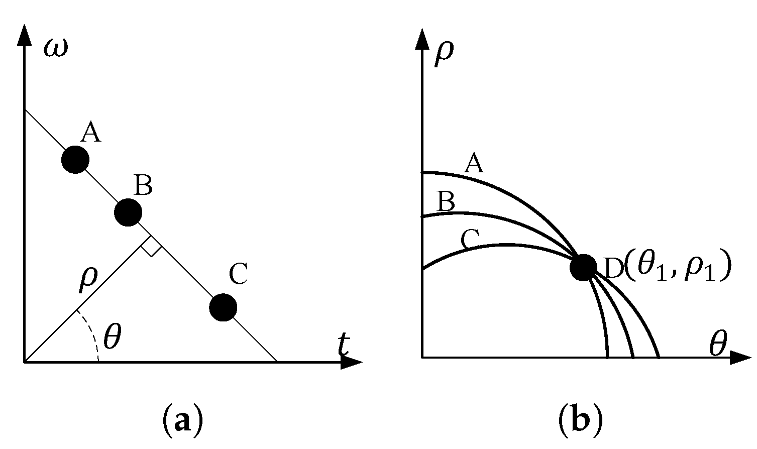
The basic principle of the Hough transform is shown in Figure 4. A straight line exists in the time–frequency space, with points A, B, and C lying on this line. In the time–frequency plane coordinate system, their coordinates can be expressed as ( t , ω ) , while in the polar coordinate system, they can be represented by ( θ , ρ ) , where ρ denotes the distance from the straight line to the origin of coordinates, and θ is the angle between the perpendicular from the origin to the straight line and the time axis t.
Figure 4b illustrates the mapping of points A, B, and C in the time–frequency space to the parameter space. The following relationship exists between ( t , ω ) and ( θ , ρ ) :
ρ = t cos ( θ ) + ω sin ( θ ) .
Equation (1) represents the curve expression corresponding to coordinate points in the time–frequency space mapped to the parameter space. Different points on the same straight line in the time–frequency space intersect at a single point in the parameter space. As shown in Figure 4b, the three curves corresponding to A, B, and C also intersect at point D. The expression of the straight line where A, B, and C lie in the original time–frequency space can be derived from the coordinates ( θ 1 , ρ 1 ) of D, namely,
ω = cot ( θ 1 ) t + ρ 1 csc ( θ 1 ) .
In Equation (18), θ 1 0 , and when θ 1 = ± π / 2 , ω = ρ 1 . In practical use, first, the step value of θ and the resolution of ρ are set to obtain a series of θ i and ρ i , respectively. A parameter space matrix H is then constructed with initial elements set to zero, where the number of rows and columns correspond to the number of previously set θ i and ρ i , respectively. By iterating through the set θ i , the Hough transform is performed on the non-zero elements ( t , ω ) of the binary matrix after edge detection according to Equation (1). After obtaining ρ i , the closest ρ i is determined and the count is incremented at the corresponding position in matrix H . Therefore, H can characterize the distribution of the parameter space curves corresponding to the feature points in the time–frequency space.
The larger the element at a certain position in H , the more parameter space curves pass through this point; the point corresponding to the maximum value is the intersection point of the curves. As previously mentioned, this intersection point corresponds to a straight line in the time–frequency space. As the proposed algorithm is adopted to improve the resolution of time–frequency analysis, concentrating energy on the IF trajectories of LFM signals and threshold filtering is performed on the edge detection results; the largest element in H represents the upper and lower bounds of the edge corresponding to the IF trajectory of the LFM signal. Therefore, local peak detection on H is required.
For K LFM components in the time–frequency space, after pre-processing the parameter space matrix H (obtained via the Hough transform) by setting an appropriate threshold, followed by maximum detection and non-maximum suppression within a reasonable neighborhood range, 2 K peak points can be searched for. These peak points follow a unified parameter set, explicitly defined as
Ω = { ( θ k upper , ρ k upper ) , ( θ k lower , ρ k lower ) | k = 1 , 2 , , K } .
In this set Ω , each LFM component corresponds to two peak points in the parameter space: one peak point ( θ k upper , ρ k upper ) for the upper boundary of its IF trajectory, and another peak point ( θ k lower , ρ k lower ) for the lower boundary. Taking the first LFM component ( k = 1 ) as an example, substituting its corresponding peak points ( θ 1 upper , ρ 1 upper ) and ( θ 1 lower , ρ 1 lower ) into the linear relationship of IF trajectory derived from the Hough transform (Equation (18)), the upper and lower bounds of its IF trajectory can be mathematically expressed as
{ ω 1 upper ( t ) = cot ( θ 1 upper ) t + ρ 1 upper csc ( θ 1 upper ) ω 1 lower ( t ) = cot ( θ 1 lower ) t + ρ 1 lower csc ( θ 1 lower ) .
In Equation (20), ω 1 upper ( t ) and ω 1 lower ( t ) are the upper and lower bounds of the IF trajectory of the first LFM component, respectively. As the energy of the actual LFM signal diffuses to both sides along the perpendicular direction of the IF trajectory, the IF estimate ω 1 ( t ) of the first LFM component can be derived as follows:
ω 1 ( t ) = ω 1 upper ( t ) + ω 1 lower ( t ) 2 .
The same applies to the remaining LFM components.

3.4. Time–Frequency Filtering

After obtaining the IF results of multiple LFMs, the de-chirping algorithm for time–frequency filtering is employed to separate individual sources. The specific calculation process is as follows:
First, for the IF IF k ( t ) of each LFM signal (where k = 1 , 2 , , K ), the phase ϕ ^ k ( t ) of each source can be estimated as follows:
ϕ ^ k ( t ) = 2 π 0 t IF k ( τ ) d τ , k = 1 , 2 , , K .
In Equation (22) ϕ ^ k ( t ) is a phase estimator specifically for LFM signals. For LFM signals, the IF is the derivative of the phase, so integrating the IF directly gives the phase. The initial phase term is omitted because it cancels out in subsequent de-chirping, not affecting results. Since LFM signals have known IF trajectories (estimated via Hough transform), making integration a simpler and more efficient method. Using the phase estimate ϕ ^ k ( t ) , de-chirping processing can be performed on the data z l k ( t ) (where l = 1 , 2 , , M ) collected by a uniform linear array with M elements spaced by d, as follows:
y l k ( t ) = z l k ( t ) e j ϕ ^ k ( t ) = ( i = 1 K e j 2 π ( l 1 ) d λ sin ( θ i ) a i ( t ) e j ϕ i ( t ) ) e j ϕ ^ k ( t ) = ( i = 1 , i K K e j 2 π ( l 1 ) d λ sin ( θ i ) a i ( t ) e j ϕ i ( t ) ) e j ϕ ^ k ( t ) + e j 2 π ( l 1 ) d λ sin ( θ k ) a k ( t ) e j ϕ i ( t ) ϕ ^ k ( t ) .
Assuming that the IF estimation is accurate, then ϕ i ( t ) ϕ ^ k ( t ) 0 , and it follows that
y l k ( t ) = ( i = 1 , i K K e j 2 π ( l 1 ) d λ sin ( θ i ) a i ( t ) e j ϕ i ( t ) ) e j ϕ ^ k ( t ) + e j 2 π ( l 1 ) d λ sin ( θ k ) a k ( t )
For y l k ( t ) , the low-frequency component LF l k ( t ) = e j 2 π ( l 1 ) d λ sin ( θ k ) a k ( t ) , whose phase is determined solely by θ k , can be obtained through low-pass filtering. x ^ l k ( t ) = LF l k ( t ) e j ϕ ^ k ( t ) is then used as the processed array data to construct the matrix X k ( t ) = [ x ^ 1 k ( t ) , x ^ 2 k ( t ) , , x ^ M k ( t ) ] T for input to the MUSIC algorithm. The calculation is performed by iterating K times and substituting the estimated IF k ( t ) at each step, thereby achieving source separation and spatial spectrum estimation.

3.5. DOA Estimation Using MUSIC

After time–frequency filtering, the covariance matrix of X k ( t ) is typically calculated through statistical averaging of the matrix in the time dimension and is expressed as follows:
R X X = 1 M X k X k H
Next, eigenvalue decomposition is performed on R X X to obtain the eigenvectors { v ^ 1 , v ^ 2 , …, v ^ M } , which are sorted in descending order according to their corresponding eigenvalues { λ 1 , λ 2 , , λ M } . As DOA estimation is performed for individual sources, the signal subspace is represented by the largest eigenvector, that is, v ^ 1 , while the noise subspace is represented by the remaining M 1 vectors. The spatial spectrum P k ( θ ) corresponding to the source can be obtained, and the DOA is estimated by the peak of P k ( θ ) using MUSIC algorithm [10]. The expression of the spatial spectrum is as follows:
P k ( θ ) = 1 ( m = 2 M | a ( θ k ) v ^ m | ) 2 .

4. Experiments and Comparisons

4.1. Two Sources

Consider two LFM signals with the following expressions, incident from angles of 5 and 5 , respectively, and received by 6 sensors:
s 1 ( t ) = e j ( 2 π ( 0.1 t + 0.15 255 t 2 ) ) s 2 ( t ) = e j ( 2 π ( 0.15 t + 0.15 255 t 2 ) ) ,
where t represents time ranging from 0 to 255.
Figure 5 shows the DOA estimation process of the proposed algorithm under the condition of SNR = 10 dB.
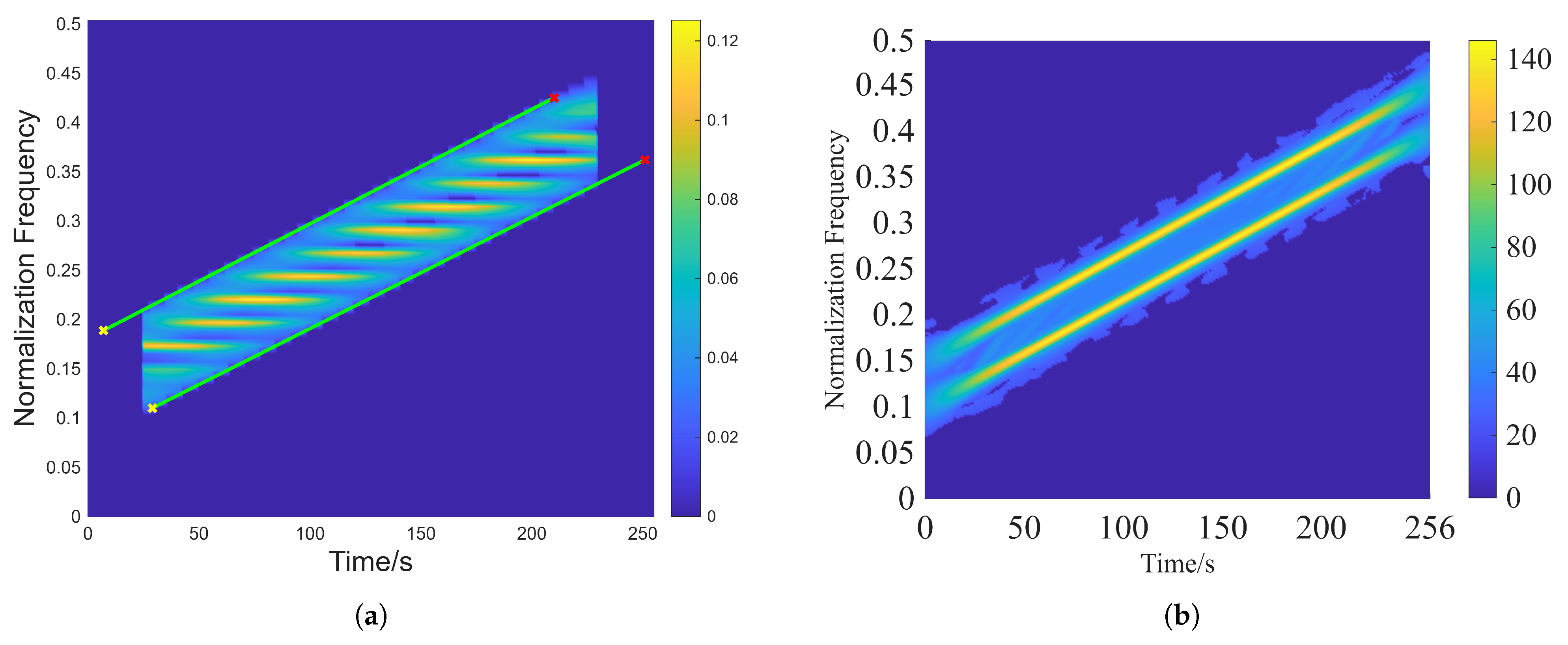
Figure 5a shows the time–frequency representation of the auto-terms of the STFD matrix constructed based on CKD. Figure 5b shows the results after the STFD matrix has undergone spatial smoothing and directional smoothing, followed by identification of the IF trajectory edges using the Hough transform. The time–frequency representation after smoothing effectively suppresses cross-terms, with energy concentrated on the IF trajectories. Meanwhile, compared with the Hough transform results of the STFT-based algorithm [16] shown in Figure 6a, the method proposed in this study, which combines QTFD and the Hough transform, successfully identifies the upper and lower edges of the two close IF trajectories.
Figure 5c shows the comparison between the IF estimation results obtained using the proposed algorithm and the theoretical values. Compared with the point selection results in Figure 6b, the proposed algorithm filters out irrelevant time–frequency points, which can improve the accuracy of the final DOA estimation. Figure 5d shows the spatial spectra and DOA estimation results constructed by the proposed algorithm, the STFT-Hough algorithm [16], and the robust spatial adaptive directional time–frequency distribution (SADTFD)-based algorithm [26]. The STFT-Hough DOA estimation algorithm exhibits distortion in the spatial spectrum due to time–frequency energy aliasing. Both the proposed algorithm and the robust SADTFD-based DOA estimation algorithm successfully estimate the DOA, but the estimation results of the proposed algorithm are closer to the theoretical values.
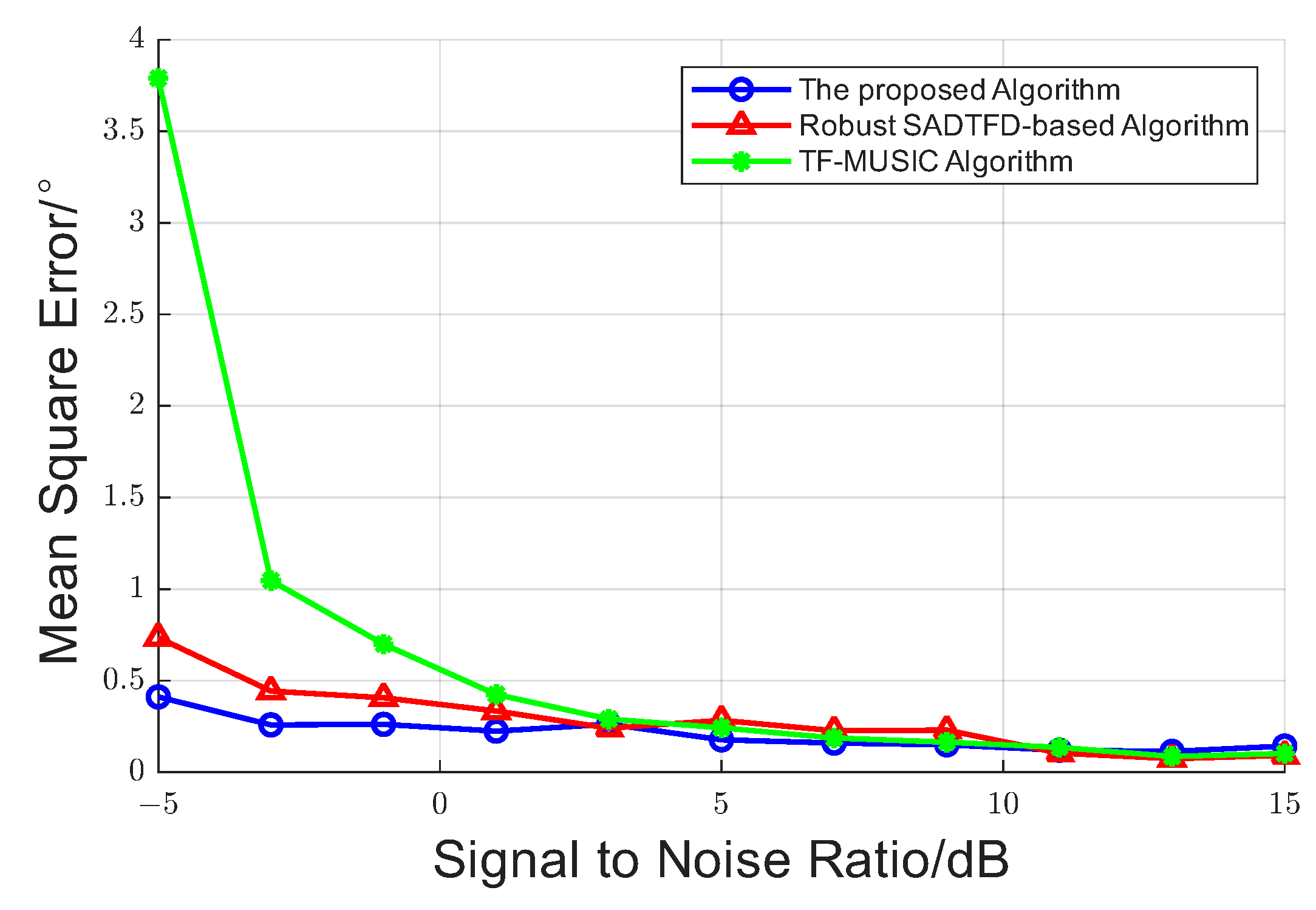
One hundred Monte Carlo simulation experiments were conducted on similar algorithms by varying the SNR from 5 to 15 dB, and the relationship between the root mean square error (RMSE) and SNR was obtained, as shown in Figure 7. The formula for calculating the RMSE is as follows:
RMSE = n = 1 N k = 1 K ( θ ^ n , k θ k ) 2 N K .
where θ ^ n , k denotes the DOA estimation value of the k-th signal source in the n-th experiment, N is the number of experiments, and K is the number of signal sources.
Figure 7 shows that when the SNR decreases to 5 dB, the traditional TF-MUSIC algorithm [28] has the lowest accuracy, while the estimation error of the proposed algorithm is reduced by approximately 43.2% compared with the robust SADTFD-based algorithm [26]. Moreover, as the SNR increases, when the SNR 5 dB, the accuracy of the proposed algorithm is still higher than that of other algorithms. In the range of 5 dB < SNR < 15 dB , the estimation errors of the three algorithms gradually converge. This experiment demonstrates that the proposed algorithm has a higher DOA estimation accuracy in low-SNR environments for two LFM signals with the same chirp rate and close initial frequencies than other algorithms.
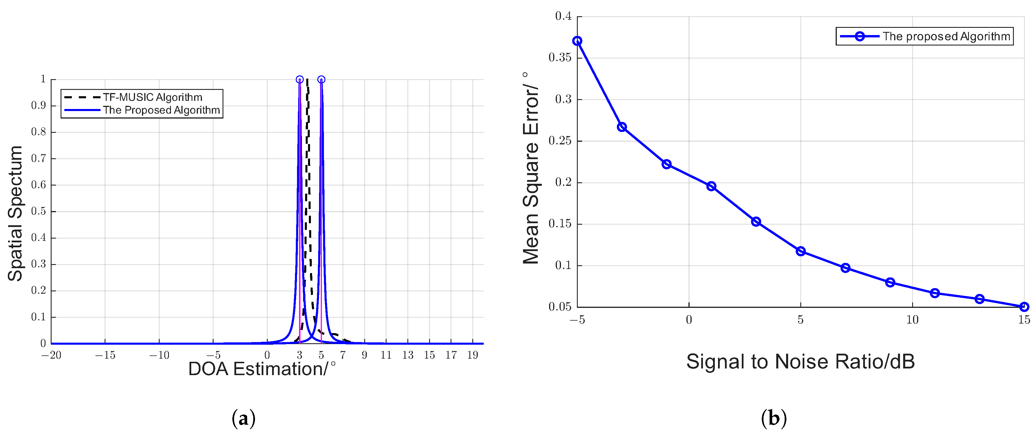
To further verify the performance of the proposed algorithm, this study still uses the two signals expressed in Equation (27). Under an environment with SNR = 10 dB, the two signals are adjusted to be incident at two close angles of 3 and 5 . After being received by ULA, the proposed algorithm is used for DOA estimation, Figure 8a shows the spatial spectrum constructed by the proposed algorithm. It can be observed that the algorithm proposed in this study estimates the DOAs of the two signal sources relatively accurately, whereas the TF-MUSIC algorithm exhibits distortion.
This study further conducts 100 simulation experiments with SNR ranging from 5 dB to 15 dB and calculates the estimation error according to Equation (28). The obtained results are shown in Figure 8b. It can be seen that as the SNR increases, the estimation accuracy gradually converges from approximately 0 . 37 to within 0 . 10 .
The traditional MUSIC algorithm suffers from the rank deficiency of the covariance matrix in underdetermined situations. As the proposed algorithm performs IF estimation individually for each signal source, it can correctly estimate DOA in underdetermined situations. Similarly, the two LFM signals in Equation (27) are received by 2 sensors in an environment with SNR = 10 dB. Figure 9 shows the spatial spectrum obtained by the proposed algorithm, indicating that the proposed algorithm successfully estimates the DOA.
Consistent with the underdetermined scenario, 100 Monte Carlo simulation experiments were conducted in which the SNR value was varied. The relationship between the RMSE and SNR is shown in Figure 10. When the SNR is <0 dB, the proposed algorithm achieves a higher accuracy compared with the ridge tracking-based algorithm [29] and the fast IF estimation-based algorithm [30]. As the SNR increases, the estimation errors of all algorithms gradually decrease and converge.

4.2. Three Sources

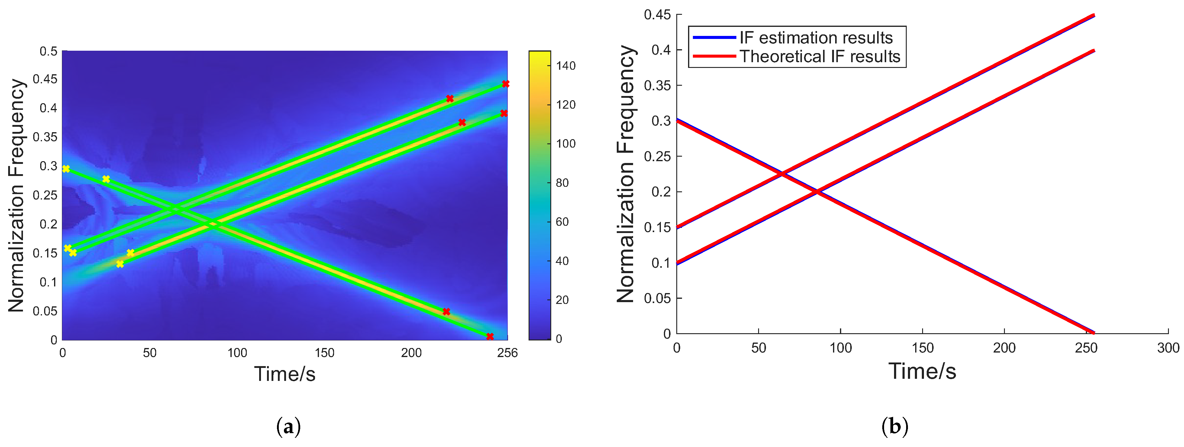
Consider three LFM signals with the following expressions, incident from angles of 5 , 5 , and 10 , respectively, received by six sensors under the condition of SNR = 10 dB:
s 1 ( t ) = e j ( 2 π ( 0.1 t + 0.15 255 t 2 ) ) s 2 ( t ) = e j ( 2 π ( 0.3 t 0.15 255 t 2 ) ) s 3 ( t ) = e j ( 2 π ( 0.15 t + 0.15 255 t 2 ) ) .
Figure 11a shows the results of constructing the STFD matrix via QTFD, followed by spatial directional smoothing and the Hough transform. Figure 11b shows the IF estimation results obtained using the proposed algorithm. The results are close to the theoretical IF trajectories.
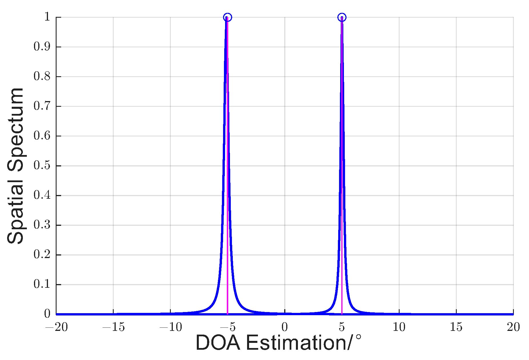
Figure 12 shows the spatial spectrum, as constructed by the proposed algorithm. In summary, the proposed algorithm can effectively handle DOA estimation for LFM signals with overlapping and close multiple IF trajectories.

4.3. Computational Complexity

To comprehensively compare the performance of algorithms similar to our proposed algorithm, their computational complexity was calculated and compared, as shown in Table 1. In Table 1, K denotes the number of signal sources, M denotes the number of array elements, L denotes the number of snapshots, and C × C denotes the size of the smoothing kernel. The computational complexity of the time–frequency analysis part of the proposed algorithm is O ( M L 2 log L ) , corresponding the “Constructing STFD matrix based on CKD” step in Figure 3. The complexity of the “Spatial smoothing and directional smoothing” step in Figure 3 is O ( M 2 C 2 L 2 ) , and Δ 1 is used to represent the complexity of “IF estimation using the Hough transform”, with Δ 1 M L 2 log L . The remaining steps in Figure 3 —“Time–frequency filtering” and “Spatial Spectrum construction using MUSIC” —contribute O ( K M L ) and O ( M 3 ) , respectively. Notably, since all the algorithms compared perform DOA estimation based on the MUSIC algorithm, the complexity of the MUSIC algorithm is not listed in Table 1.
Compared with the STFT-Hough algorithm, the proposed algorithm is nonlinear and therefore has a higher complexity [16]. In contrast to the complexity of O ( L 3 ) of the Viterbi-based algorithm adopted in [22], the complexity of the algorithm using the Hough transform for IF estimation is significantly lower. The fast IF estimation-based algorithm used in [30] involves running the fast Fourier transform (FFT) algorithm F times using a spectral analysis window of length W for P effective spectral points. The complexity of this algorithm, therefore, depends on the size of its selected parameters, F, W, and P. These parameters satisfy the relationship P , W , F L 2 ; thus, the complexity of this algorithm is significantly lower than that of the algorithm used in [22]. Similarly, the complexity of the robust SADTFD-based algorithm used in [26] is slightly lower than that of the proposed algorithm.

5. Conclusions

In conclusion, to estimate the DOA of multiple LFM signals, this study proposed an algorithm based on QTFD and the Hough transform. The algorithm analyzes time–frequency features through QTFD, performs source separation and IF estimation using the Hough transform, and finally constructs the spatial spectrum with the MUSIC algorithm to obtain the DOA estimation results. Compared with the DOA-estimation algorithm based on STFD matrices constructed by STFT, the proposed algorithm has a higher resolution, supports simultaneous processing of multiple LFM signals with the same chirp rates and close initial frequencies and thus expands the potential application scenarios. Compared with the DOA-estimation algorithm based on STFD matrices constructed by QTFD, the proposed algorithm adopts the Hough transform to further improve the IF estimation accuracy in low-SNR environments, thereby enhancing the accuracy and robustness of the DOA estimation algorithm. Moreover, this algorithm is applicable to both overdetermined and underdetermined cases.

Author Contributions

Conceptualization, G.W.; methodology, G.W. and H.F.; software, G.W. and Z.M.; validation, G.W. and H.F.; writing—original draft preparation, G.W.; writing—review and editing, Z.M. and B.Z.; project administration, B.Z. All authors have read and agreed to the published version of the manuscript.

Funding

This research received no external funding.

Data Availability Statement

The original contributions presented in this study are included in the article material. Further inquiries can be directed to the corresponding author.

Conflicts of Interest

The authors declare no conflicts of interest.

References

  1. Joshi, S.K.; Baumgartner, S.V.; da Silva, A.B.C.; Krieger, G. Direction-of-Arrival Angle and Position Estimation for Extended Targets Using Multichannel Airborne Radar Data. IEEE Geosci. Remote Sens. Lett. 2022, 19, 4022705. [Google Scholar] [CrossRef]
  2. Sümen, G.; Kurt, G.K.; Görçin, A. A Novel LFM Waveform for Terahertz-Band Joint Radar and Communications over Inter-Satellite Links. In Proceedings of the GLOBECOM 2022—2022 IEEE Global Communications Conference, Rio de Janeiro, Brazil, 4–8 December 2022; pp. 6439–6444. [Google Scholar] [CrossRef]
  3. Komeylian, S.; Mihovska, A.D.; Sarkar, M.; Paolini, C. A FFNN-Based System for the DoA Estimation in 6G Massive Wireless Communications: Analysis and Evaluation. In Proceedings of the 2024 IEEE Wireless Communications and Networking Conference (WCNC), Dubai, United Arab Emirates, 21–24 April 2024; pp. 1–6. [Google Scholar] [CrossRef]
  4. Latif, M.; Sanei, S.; Chambers, J.; Shoker, L. Localization of abnormal EEG sources using blind source separation partially constrained by the locations of known sources. IEEE Signal Process. Lett. 2006, 13, 117–120. [Google Scholar] [CrossRef]
  5. Hachad, L.; Mrabti, F.; Ghennioui, H.; Zouak, M. A Time Frequency Tensor Framework for DOA Estimation: Application to MIMO Systems. In Proceedings of the 2019 International Conference on Wireless Networks and Mobile Communications (WINCOM), Fez, Morocco, 29 October–1 November 2019; pp. 1–6. [Google Scholar] [CrossRef]
  6. Jia, W.; Cao, Y.; Zhang, S.; Wang, W.Q. Detecting High-Speed Maneuvering Targets by Exploiting Range-Doppler Relationship for LFM Radar. IEEE Trans. Veh. Technol. 2021, 70, 2209–2218. [Google Scholar] [CrossRef]
  7. Mulinde, R.; Kaushik, M.; Dissanayake, D.W.; Attygalle, M.; Chan, T.; Ho, S.W.; Aziz, S.M. DOA estimation of wideband LFM RADAR signals. In Proceedings of the 2019 International Radar Conference (RADAR), Toulon, France, 23–27 September 2019; pp. 1–6. [Google Scholar] [CrossRef]
  8. Mercuri, M.; Lorato, I.R.; Liu, Y.H.; Wieringa, F.; Hoof, C.V.; Torfs, T. Vital-sign monitoring and spatial tracking of multiple people using a contactless radar-based sensor. Nat. Electron. 2019, 2, 252–262. [Google Scholar] [CrossRef]
  9. Gilles Yowel, M.M.; Oh, D.H.; Kim, H.J.; Jeong, B.J.; Han, J.H. SNR Improvement for Heart Rate Estimation Using mmWave 79 GHz FMCW MIMO Radar. In Proceedings of the 2023 International Symposium on Electromagnetic Compatibility—EMC Europe, Krakow, Poland, 4–8 September 2023; pp. 1–5. [Google Scholar] [CrossRef]
  10. Schmidt, R. Multiple emitter location and signal parameter estimation. IEEE Trans. Antennas Propag. 1986, 34, 276–280. [Google Scholar] [CrossRef]
  11. Rao, B.; Hari, K. Performance analysis of Root-Music. IEEE Trans. Acoust. Speech Signal Process. 1989, 37, 1939–1949. [Google Scholar] [CrossRef]
  12. Roy, R.; Kailath, T. ESPRIT-estimation of signal parameters via rotational invariance techniques. IEEE Trans. Acoust. Speech Signal Process. 1989, 37, 984–995. [Google Scholar] [CrossRef]
  13. Belouchrani, A.; Amin, M. Blind source separation based on time-frequency signal representations. IEEE Trans. Signal Process. 1998, 46, 2888–2897. [Google Scholar] [CrossRef]
  14. Belouchrani, A.; Amin, M.G.; Thirion-Moreau, N.; Zhang, Y.D. Source Separation and Localization Using Time-Frequency Distributions. IEEE Signal Process. Mag. 2013, 30, 97–107. [Google Scholar] [CrossRef]
  15. Heidenreich, P.; Cirillo, L.A.; Zoubir, A.M. Morphological image processing for FM source detection and localization. Signal Process. 2009, 89, 1070–1080. [Google Scholar] [CrossRef]
  16. Zhang, X.; Zhang, W.; Yuan, Y.; Cui, K.; Xie, T.; Yuan, N. DOA estimation of spectrally overlapped LFM signals based on STFT and Hough transform. EURASIP J. Adv. Signal Process. 2019, 2019, 58. [Google Scholar] [CrossRef]
  17. Yang, Y.; Peng, Z.K.; Dong, X.J.; Zhang, W.M.; Meng, G. General Parameterized Time-Frequency Transform. IEEE Trans. Signal Process. 2014, 62, 2751–2764. [Google Scholar] [CrossRef]
  18. Xiang-qian, S.; Zhan, F.; Qing, L. A method of target DOA estimation based on correlation integral and cross spectrum WVD. Tech. Acoust. 2015, 34, 23–28. [Google Scholar] [CrossRef]
  19. Abed, M.; Belouchrani, A. Performance analysis and computational cost evaluation of high-resolution time-frequency distributions derived from compact support time-lag kernels. Digit. Signal Process. 2018, 78, 1–19. [Google Scholar] [CrossRef]
  20. Ali Khan, N.; Ali, S.; Jansson, M. Direction of arrival estimation using adaptive directional time-frequency distributions. Multidimens. Syst. Signal Process. 2018, 29, 503–521. [Google Scholar] [CrossRef]
  21. Cui, K.; Chen, X.; Huang, J.; Yuan, N. DOA estimation of multiple LFM sources using a STFT-based and FBSS-based MUSIC algorithm. Radioengineering 2017, 26, 1126–1137. [Google Scholar] [CrossRef]
  22. Zhang, J.; Li, T.; He, Q.; Peng, Z. DOA Estimation of Nonstationary and Close-Spaced Sources Based on Unified Parameterized Model. IEEE Sensors J. 2023, 23, 21599–21609. [Google Scholar] [CrossRef]
  23. Xia, X.; Yu, F.; Liu, C.; Zhao, J.; Wu, T. Time-Frequency Image Enhancement of Frequency Modulation Signals by Using Fully Convolutional Networks. In Proceedings of the 2018 15th International Conference on Control, Automation, Robotics and Vision (ICARCV), Singapore, 18–21 November 2018; pp. 1472–1476. [Google Scholar] [CrossRef]
  24. Eranti, P.K.; Barkana, B.D. An Overview of Direction-of-Arrival Estimation Methods Using Adaptive Directional Time-Frequency Distributions. Electronics 2022, 11, 1321. [Google Scholar] [CrossRef]
  25. Cohen, L. Time-Frequency Analysis: Theory and Applications; Prentice-Hall, Inc.: Upper Saddle River, NJ, USA, 1995. [Google Scholar]
  26. Khan, N.A. Robust Spatial Time-Frequency Distributions for DOA Estimation Using Spatial Averaging and Directional Smoothing. Signal Process. 2021, 180, 107897. [Google Scholar] [CrossRef]
  27. Duda, R.O.; Hart, P.E. Use of the Hough transformation to detect lines and curves in pictures. Commun. ACM 1972, 15, 11–15. [Google Scholar] [CrossRef]
  28. Belouchrani, A.; Amin, M. Time-frequency MUSIC. IEEE Signal Process. Lett. 1999, 6, 109–110. [Google Scholar] [CrossRef]
  29. Khan, N.A.; Ali, S.; Mohammadi, M.; Haneef, M. Direction of arrival estimation of sources with intersecting signature in time-frequency domain using a combination of IF estimation and MUSIC algorithm. Multidimens. Syst. Signal Process. 2020, 31, 549–567. [Google Scholar] [CrossRef]
  30. Khan, N.A.; Ali, S.; Choi, K. An Efficient Direction of Arrival Estimation Algorithm for Sources with Intersecting Signature in the Time-Frequency Domain. Appl. Sci. 2021, 11, 1849. [Google Scholar] [CrossRef]
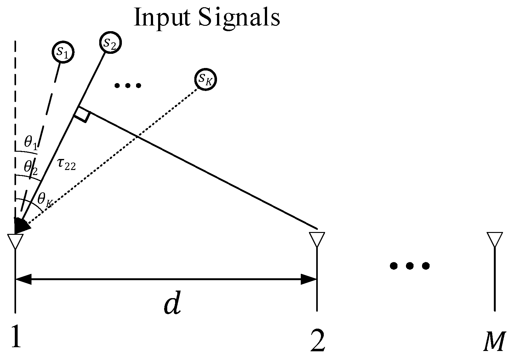
Figure 1. ULA model.
Applsci 15 10264 g001
Figure 2. Comparison between the processing results obtained using the STFT and WVD algorithms for two LFM signals with the same chirp rate and close initial frequencies: (a) Three-dimensional processing results of the STFT algorithm. (b) Three-dimensional processing results of the WVD algorithm. (c) time–frequency plane processed by the STFT algorithm. (d) Time–frequency plane processed by the WVD algorithm.
Applsci 15 10264 g002
Figure 3. ProposedDOA estimation algorithm.
Applsci 15 10264 g003
Figure 4. Schematic of the coordinate spaces before and after the Hough transform: (a) Time–frequency space before the Hough transform. (b) Parameter space after the Hough transform.
Applsci 15 10264 g004
Figure 5. DOA estimation process of the proposed algorithm: (a) Time–frequency analysis results based on the CKD algorithm. (b) Results of time–frequency analysis after spatial and directional smoothing, as well as results of IF trajectory edge recognition via the Hough transform. (c) Comparison between the IF estimation results obtained using the proposed algorithm and the theoretical values. (d) Comparison between the spatial spectra constructed by the proposed algorithm and other similar algorithms.
Applsci 15 10264 g005
Figure 6. Time–frequency analysis results of other similar algorithms: (a) Time–frequency analysis results of the DOA estimation algorithm based on the STFT algorithm. (b) Time–frequency analysis results of the DOA estimation algorithm using the robust SADTFD algorithm.
Applsci 15 10264 g006
Figure 7. Accuracy comparison of DOA estimation algorithms in overdetermined situations.
Applsci 15 10264 g007
Figure 8. Time–frequency analysis results of other similar algorithms: (a) Comparison between the spatial spectra constructed by the proposed algorithm and TF-MUSIC algorithm for two closely spaced LFM signals in the angular domain. (b) Accuracy of the proposed algorithm for two closely spaced LFM signals in the angular domain under different SNR conditions.
Applsci 15 10264 g008
Figure 9. Spatial spectrum of the proposed DOA estimation algorithm in underdetermined situations.
Applsci 15 10264 g009
Figure 10. Accuracy comparison of DOA estimation algorithms in underdetermined situations.
Applsci 15 10264 g010
Figure 11. Process of the proposed algorithm for three LFM signals: (a) Results of the time–frequency analysis based on QTFD after spatial smoothing and directional smoothing, and results of IF trajectory edge recognition via the Hough transform. (b) Comparison between the IF estimation results obtained using the proposed algorithm and the theoretical values.
Applsci 15 10264 g011
Figure 12. Comparisonbetween the spatial spectra constructed by the proposed algorithm and other similar algorithms for three LFM signals.
Applsci 15 10264 g012
Table 1. Comparison of the computational complexity.
AlgorithmComplexity
STFT-Hough algorithm [16] O ( K M L 2 log L + K Δ 1 + K M L )
Robust SADTFD-based algorithm [26] O ( M L 2 log L + M 2 C 2 L 2 )
Fast IF estimation-based algorithm [30] O ( 3 K M P W L + K M F W log W + K L W M )
Viterbi-based algorithm [22] O ( K M L 2 log L + L 3 + K M L )
The proposed algorithm O ( M L 2 log L + M 2 C 2 L 2 + K Δ 1 + K M L )
Disclaimer/Publisher’s Note: The statements, opinions and data contained in all publications are solely those of the individual author(s) and contributor(s) and not of MDPI and/or the editor(s). MDPI and/or the editor(s) disclaim responsibility for any injury to people or property resulting from any ideas, methods, instructions or products referred to in the content.