Abstract
Spaceborne Synthetic Aperture Radar (SAR) is extensively used in maritime surveillance due to its ability to monitor vast oceanic regions regardless of weather conditions and sun illumination. Over the years, numerous automatic ship detection algorithms have been developed, utilizing either single-polarimetric data (i.e., intensity) or leveraging additional information provided by polarimetric sensors. One of the main challenges in automatic ship detection using SAR is that sea clutter, influenced primarily by sea conditions and image acquisition angles, can exhibit strong backscatter, reducing the signal-to-clutter ratio (that is, the contrast) between ships and their surroundings. This leads inevitably to detection errors, which can be either false alarms or miss-detections. A potential solution to this issue is to develop methodologies that suppress backscattered signals from the sea while preserving the radar returns from ships. In this work, we analyse a contrast enhancement method which is designed to suppress unwanted sea clutter while preserving signals from potential ships. A key advantage of this method is that it is fully analytical, eliminating the need for numerical optimization and enabling the rapid generation of an enhanced image better suited for automatic detection. This technique, based on polarimetric orthogonality, was originally formulated for quad-polarimetric data, and here the adaptation for dual-polarimetric SAR images is also detailed. To demonstrate its effectiveness, a comprehensive set of results using both quad- and dual-polarimetric images acquired by various sensors operating at L-, C-, and X-band is presented.
1. Introduction
Synthetic Aperture Radar (SAR) imagery is widely used in maritime surveillance, providing a robust and reliable solution for monitoring vast oceanic areas. Unlike optical sensors, which are limited by weather conditions and daylight, SAR systems actively emit microwave signals that penetrate clouds, fog, and precipitation, making them operational in all weather and lighting conditions. This capability is particularly critical for maritime surveillance, where oceans often experience dynamic and unpredictable environments. SAR images are used for a wide range of applications, including detecting and tracking ships, monitoring illegal activities such as smuggling and unauthorized fishing, and supporting search-and-rescue operations. The high-resolution imaging capabilities of SAR, combined with its ability to cover extensive areas, provide consistent and actionable insights, making it an indispensable asset for both civilian and defence-related maritime operations.
A traditional and automatic ship detection method with SAR images is the one based on the well-known Constant False Alarm Rate (CFAR) and its variants [1,2,3,4,5,6]. The fundamental idea of a CFAR detector consists in taking advantage of the intensity difference between the ship and the surrounding sea clutter. Since ships appear as bright targets in the SAR image, with a stronger radar response compared to sea clutter, CFAR methods aim to statistically model the background clutter (the sea/water) to effectively distinguish each ship from its surroundings. In other words, CFAR detectors assume that the statistical distribution of the sea clutter is known and use it to threshold the image to distinguish the ship from the background. Different statistical models have been proposed, including the Weibull-, Log-normal-, K-, or Gamma-distributed models [7,8]. Major advantages of CFAR-based detectors are their fast processing speed and implementation simplicity. However, they are sometimes limited in complex scenarios where there is not enough contrast between the target (ship) and the background clutter, or for the detection of ships across multiple scales. Also, CFAR detection algorithms involve multiple processing parameters, the generalization of which is, normally, unfeasible. Such parameters are the dimensions of the search window and the probability of a false alarm, among others [4].
In recent years, with the inclusion of deep learning techniques for the exploitation of SAR data across a wide range of applications [9], sophisticated ship detection methods based on neural networks have emerged as a promising solution. A significant number of studies have demonstrated that advanced methods based on deep learning achieve similar or even higher detection accuracies compared to traditional algorithms. An extensive review of ship detection methods for SAR images based on deep learning can be found in the following references [10,11,12,13,14,15]. An advantage of Artificial Intelligence (AI)-based detectors is their data-driven and non-parametric nature, meaning they do not require manual configuration of detection parameters. However, training these models effectively necessitates a large dataset to provide the neural network with enough information to learn meaningful features from target ships. Generating such datasets presents considerable difficulties because of the extensive number of SAR images that need to be processed and analysed (using conventional methods). Additionally, manual intervention is often required to ensure the dataset is accurately curated, further complicating the process of preparing reliable training data for neural network models.
However, regardless of the detection method used, processing SAR images for automatically detecting ships poses significant challenges. This is mainly due to the following aspects. Firstly, the radar response of both ships and the sea surface is highly dependent on the sensor’s imaging geometry. It is well known that the incidence angle between the radar beam and the surface influences the amount of signal that is backscattered to the sensor. In this regard, steep incidence angles lead to a higher backscatter intensity, particularly from the sea, which reduces the contrast between the ship and its surroundings. On the contrary, shallow incidence angles benefit from a reduced return from the sea surface, resulting in a higher image contrast, but the occurrence of azimuth and range ambiguities increases [16]. Secondly, natural phenomena such as ocean currents, waves, wind, or other meteorological conditions can also impact the backscattering properties of the sea surface, leading to a reduction of image contrast and limiting the application of automatic ship detection methods [16]. This decrease in algorithm performance causes inevitably the appearance of either false positives (i.e., wrong detections) or miss-detections (i.e., undetected ships). Additionally, another important issue to consider is that vessels might be moving during the acquisition of the SAR image. Since SAR systems depend on the coherent processing of transmitted and received electromagnetic signals over time, vessel movement inevitably causes blurriness and defocusing effects, further complicating automatic detection. Reducing the impact of target movement requires specific processing to be applied before any detection technique. Different methods aim at reducing these undesired effects caused by the target’s motion, including Phase Gradient Autofocus algorithms [17], Inverse SAR (ISAR) processing [18], or recently published and more sophisticated techniques based on 3D Inverse Interferometric SAR (3D InISAR) [19] and its polarimetric extension [20].
To mitigate the impact of the previously mentioned issues, specifically the ones that cause a lack of contrast between vessels and surrounding sea clutter, a common strategy involves applying preprocessing to the data to optimize subsequent detection. In this context, leveraging the multiple polarizations provided by modern SAR sensors has gained significant attention and has proven effective in enhancing vessel detection capabilities using SAR images [21,22,23,24]. A sub-optimal solution is to process the VH polarization (if available), as it is expected to provide greater contrast between vessels and sea areas [25]. Another approach, when quad-polarimetric data are available, is to subtract the VV component from the image SPAN [26], given that the sea response is generally stronger in this channel. Alternatively, some methods proposed different polarimetric optimizations with the goal of suppressing sea clutter while preserving the polarimetric signatures of vessels, thereby improving subsequent detection [27,28,29,30]. More details about different polarimetric methods employed to improve vessel detection capabilities are given in the Discussion section (Section 5) of this manuscript.
In this paper, we propose the use of a recently published and innovative polarimetric optimization [31] as a preprocessing step to enhance image contrast, thereby improving the application of target detection techniques. The core idea of this method consists in exploiting target orthogonality leveraging all available polarimetric information. By manually selecting a reference pixel (or patch) containing an undesired feature (e.g., located at the sea), image data are projected onto an orthogonal space that cancels the selected feature and enhances others (i.e., ships). Consequently, the polarimetric optimization can be generally applied to the detection of desired targets that are located on difficult environments. Here, we focus on the detection of vessels imaged by SAR sensors at different frequency bands, and we analyse the eventual improvement that the optimization provides for different combinations of polarimetric channels. Special focus is placed on the performance of the different combinations of channels found in dual-pol systems.
Furthermore, the study evaluates the optimization performance using SAR data acquired at three frequency bands (L-, C-, and X-band) to better demonstrate the effectiveness of the contrast enhancement method. These three bands are commonly used for vessel detection [2,15,25], each offering distinct advantages and limitations. The L-band (1–2 GHz) is well suited for detecting large vessels, as it provides better penetration through clouds and rain, making it effective in adverse weather conditions and rough seas. However, spatial resolution is normally lower compared to the other bands. The C-band (4–8 GHz) offers a balance between resolution and sensitivity to the ocean surface, making it ideal for detecting medium to large vessels in various sea states. It is widely used in SAR systems like Sentinel-1. The X-band (8–12 GHz) provides the highest resolution, enabling the detection of smaller vessels and fine details; however, it is more sensitive to sea surface roughness and weather conditions, which can limit its effectiveness in rough seas. It is very important to note that the goal of this work is to demonstrate how this contrast enhancement technique can be utilized with dual- and quad-pol data acquired at different bands to eventually improve the performance of ship detectors on SAR images. Therefore, we do not propose a new ship detection method but instead focus on a pre-processing algorithm based on polarimetry for enhancing the performance of any ship detector. The contributions of this study are therefore focused on three aspects not treated in [31] when the original quad-pol formulation was proposed, namely, the following:
- Evaluation of the contrast optimization using polarimetric SAR images acquired by multiple sensors operating at different frequency bands: L-, C-, and X-band.
- Proposal of a formulation for the dual-polarimetric case (which is not detailed in the original formulation [31]), which will allow us to compare the optimization using both dual- and quad-polarimetric images.
- Comparison of the performance provided by different combinations of polarimetric channels in the dual-pol case.
2. Theory: Rank-1 Polarimetric Contrast Enhancement for Ship Detection
The general formulation employed in this work is detailed in [31], in which the polarimetric coherency matrix formalism was used. In this study, we aim at assessing the performance for quad-pol and dual-pol data, so we have adapted the expressions to the polarimetric covariance matrix, since the formulation in the dual-pol case is easier with the covariance matrix than with the coherency matrix. It is important to note that the final results for the quad-pol case are numerically equivalent, regardless of the matrix formalism, as the two matrices can be converted into each other by using an unitary transformation.
2.1. Quad-Polarimetric Case
The data contained at each pixel of a quad-pol image can be expressed using a target vector as follows [32]:
where the superscript T denotes transposition. The values represent the single-look complex (SLC) data at the polarimetric channel measured by transmitting polarization P and receiving polarization Q. In this expression, reciprocity is assumed (i.e., ), and the factor is used to preserve the total received power.
From the SLC data, the polarimetric covariance matrix is estimated, resulting in the following:
where ∗ denotes complex conjugate, and is the estimation operator, which is implemented using a speckle filter (e.g., a spatial low-pass filter).
Once the covariance matrix is estimated for each pixel, the algorithm starts by applying an eigenvector expansion of the covariance matrix, which always has real, non-negative eigenvalues, and orthogonal eigenvectors as shown in the following equation:
where are the eigenvalues, and denote the eigenvectors.
The first step of the algorithm consists in computing a new complete image which corresponds to the rank-1 covariance matrix formed by using only the largest eigenvalue/eigenvector obtained in (3), i.e.,
The second step of the method consists in selecting a reference pixel or patch (group of pixels) located in the area that we want to remove or mitigate, e.g., on the sea surface for a ship detection application.
The orthogonality of the eigenvectors implies that the first eigenvector of the reference pixel, , defines an orthogonal space, which is formed by the second and third eigenvectors, i.e., and . In the quad-pol case, the geometrical interpretation is simple: the orthogonal space is a two-dimensional plane formed by the second and third eigenvectors. Within that plane, one can measure the radar response provided by any linear unitary combination of the two eigenvectors—i.e.,
where and are two angles used to cover any possible combination, and .
In fact, it is possible to find the maximum received echo (backscattered power) at each pixel of the rest of the image (outside the reference patch) by properly selecting these two angles. The optimum values of these two angles are as follows [31]:
where and are the projections of the second and third eigenvectors of the reference patch onto the rank-1 value of the pixel (see Equation (4)). In other words,
Therefore, we can then construct, for every pixel in an image, an optimum detection channel, D, as shown in (10). This channel, D, will have the maximum amplitude possible, constrained to the null space of the reference vector [31]:
2.2. Dual-Polarimetric Case
In the dual-pol case, the images contain two of the four possible combinations of transmitted and received polarizations. Most dual-pol systems employ one polarization in transmission (either H or V) and receive both (H and V). That operation mode preserves the same spatial coverage (swath) of a single-pol system. In the case of TerraSAR-X, TanDEM-X, and PAZ sensors, their operation enables the coherent acquisition of the two copolar channels, i.e., and , at the expense of reducing the swath to half of the single-pol configuration. Therefore, there exist three possible pairs of polarimetric channels to form the target vector:
In any case, with the dual-pol target vector, we can form the 2 × 2 polarimetric covariance matrix for each pixel as follows:
This matrix can be decomposed in eigenvalues/vectors, resulting in the following:
And we can form a rank-1 image, denoted also as , using only the largest eigenvalue/vector, as in Equation (4).
In the dual-pol case, the space orthogonal to the first eigenvector is not a two-dimensional plane, but it is just the direction (or line) defined by the second eigenvector. As a result, the best channel to minimise the response from the reference patch is defined by the second eigenvector of the reference patch, . Consequently, the optimum image is generated by projecting every pixel of the rank-1 image, , onto the second eigenvector of the reference patch—i.e.,
3. Datasets
The polarimetric contrast enhancement method is evaluated with images acquired by different polarimetric SAR sensors over the ocean, with the presence of multiple ships with variable dimensions. The list of images, including relevant details for each sensor, is shown in Table 1.

Table 1.
Characteristics of the polarimetric images used in this study.
We first processed an L-band quad-pol image acquired by ALOS-1 (Advanced Land Observation Satellite) over Tokyo Bay (Japan). We also processed a quad-pol image acquired at the C-band by Radarsat-2 covering the city and the coast of Barcelona (Spain). Additionally, we used dual-pol images gathered by the PAZ SAR satellite in the X-band near the coast of Rio Grande (Brazil). To specifically evaluate the performance of the contrast enhancement method on dual-pol data at the X-band, we processed three PAZ images acquired over the same region with different polarization combinations and on different dates. For additional insights with dual-pol data, we manually selected two channels (from the four available) from the quad-pol images of ALOS-1 and Radarsat-2, enabling further comparison of dual-pol modes at other frequency bands. Additionally, we present an example of polarimetric optimization applied to a dual-pol Sentinel-1 image acquired over the Strait of Gibraltar. Although Sentinel-1 operates at the C-band, like Radarsat-2, its freely available and globally accessible data deserve special consideration, as the satellite is widely used for maritime surveillance. Moreover, since access to commercial satellite imagery is generally more restricted for scientific purposes, including an example based on a free dataset could facilitate further research in this field. This diversity in terms of sensors, frequency bands, and polarizations allows for a rich and complete analysis of the contrast enhancement method.
All images were acquired with mid-to-low (i.e., steep) incidence angles (ranging between 25° and 33°; see Table 1). Therefore, the backscattered signals coming from the sea surface are expected to be considerably high, and the benefits of the contrast enhancement can be better evaluated.
All channels of the SLC images were radiometrically calibrated to the backscattering coefficient (). Then, as the starting point of the contrast enhancement for both the quad- and dual-pol cases, the covariance matrix was generated from the calibrated SLC images. In all cases, the polarimetric covariance matrices were estimated using a 3 × 3 boxcar filter (moving average). Note that a small filtering window was used to reduce speckle without significantly degrading the original spatial resolution of the data, as excessive smoothing could hamper the detection of ships (especially small ones).
Figure 1 shows a false colour composite of each processed image, which corresponds to specific Regions of Interest (RoIs) within the full scenes. As can be seen in the RGB images, all ships exhibit specific polarimetric responses compared to their surrounding sea areas. This provides a simple way to visualize polarimetric diversity with the naked eye and demonstrates that polarimetry can be effectively exploited to develop sophisticated detection methods that leverage the additional information provided by polarimetric sensors. Actually, as detailed in [25], detection methods utilizing polarimetry, whether based on quad- or dual-polarimetric images, outperform those relying solely on the processing of single-channel intensities.
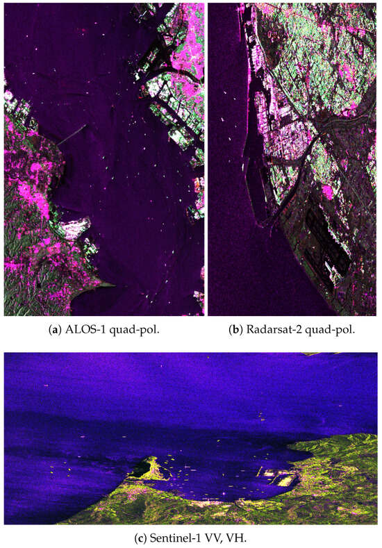
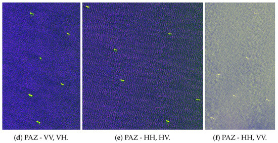
Figure 1.
RGB false colour images formed with the backscattering coefficients of each available polarimetric channel. (a,b) ALOS-1 and Radarsat-2 quad-polarimetric images with R = HH, G = HV, B = VV. (c,d) Sentinel-1 and PAZ dual-pol image with R = VV, G = VH, B = VV/VH. (e) PAZ dual-pol image with R = HH, G = HV, B = HH/HV. (f) PAZ dual-pol image with R = HH, G = VV, B = HH/VV.
In the following subsections, we present a wide variety of results derived from the processing of the different polarimetric SAR images previously introduced. In all cases, the most important aspect here consists in showing how the polarimetric preprocessing allows us to obtain a new SAR image which is more suitable for vessel detection purposes.
The starting point of the contrast enhancement for both the quad- and dual-polarimetric cases consists in generating the covariance matrix from the original SLC images. In all cases, the polarimetric covariance matrices are estimated using a 3 × 3 boxcar filter (moving average). Note that a small filtering window is used to reduce speckle without significantly degrading the original spatial resolution of the data, as excessive smoothing could hamper the detection of ships (especially small ones).
4. Results
4.1. Results with Quad-Polarimetric Data
Figure 2 shows the results obtained with the quad-pol ALOS-1 dataset. Figure 2a,b represent the intensity of channels HH and HV, respectively, which are commonly employed as conventional detection channels. A lot of ships are clearly visible throughout the scene. As expected, the HV channel exhibits higher contrast between vessels and their surroundings compared to HH [25,33,34]. However, the response of some ships in HV is weaker than in HH, which might make their detection difficult. A drawback of the HH polarization is its higher signal level from the sea areas surrounding the vessels, which reduces the contrast (i.e., the signal-to-clutter ratio) between the vessels and the sea, thus limiting the application of automatic detection techniques to that channel.
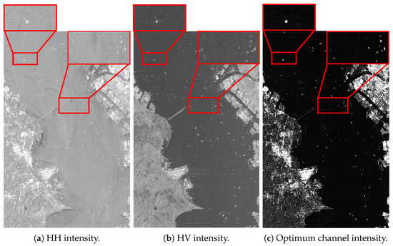
Figure 2.
Results with L-band quad-pol image acquired over Bay of Tokyo (Japan) by ALOS-1. All figures represent image intensity in logarithmic scale ranging from −35 to 0 dB.
By manually selecting one the sea pixels as reference, we obtain the optimum image shown in Figure 2c. It is clearly seen that sea clutter level is drastically reduced and, simultaneously, signal level coming from the ships is increased. As an additional remark, note that the contrast between the urban areas and vegetated areas around the Bay of Tokyo is also improved.
The improvement can also be visualized in Figure 3, which shows a range transect passing through the ship depicted in the magnified region at the top of Figure 2. On the one hand, by comparing the transects for the HH and optimum channels (blue and red plots), we observe that in the optimum channel, the ship intensity is approximately 3.5 dB higher, while (simultaneously) the sea clutter intensity is notably lower, dropping from around −8 dB to −40 dB. On the other hand, a similar effect is observed when comparing the transects corresponding to the optimum and HV channels (red and green plots, respectively). In this case, the ship intensity is about 12 dB higher, while the sea clutter intensity is observed to be 28 dB lower.
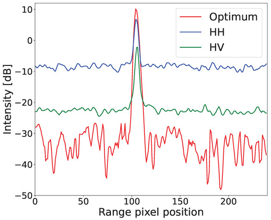
Figure 3.
Range transects through ship shown in magnified region in upper part of Figure 2, corresponding to L-band quad-pol ALOS-1 image over Bay of Tokyo.
The values of the signal-to-clutter ratio between the same ship and its surrounding background clutter are detailed in Table 2. The optimum channel exhibits the largest ratio, which indeed benefits the application of any vessel detection algorithm compared to the use of HH or HV. In the specific case of using a CFAR detector, the higher the signal-to-clutter ratio (equivalently, the higher the contrast) the more accurate detection of vessels with any value of the probability of a false alarm.
Table 2.
Signal-to-clutter ratio between ship shown in upper part of Figure 2 and its surrounding sea clutter for different polarimetric channels.
The second example corresponds to the quad-polarimetric image of Radarsat-2 acquired over Barcelona. The results are shown in Figure 4. As in the previous example, the steep incidence angle of the acquisition causes a strong response of the sea surface, particularly evident in the HH polarization, as depicted in Figure 4a. This results in a reduced signal-to-clutter ratio (contrast) between ships and their surrounding background, thereby limiting the effectiveness of detection techniques. HV provides again higher contrast than HH. However, upon closer inspection of the ships, their response appears to be scattered (or dispersed) across a wider area, as shown in the magnified region of Figure 4. In the optimum image represented in Figure 4c, we observe a clear cancellation of the signal coming from the sea surface, as well as an improved contrast between each vessel and its surrounding area. Figure 5 shows an azimuth (vertical) transect through the leftmost ship that appears in Figure 4 (highlighted with the red circle). Here, we observe that the HH polarization exhibits higher backscatter values for both the sea and the vessel (as previously stated), with an intensity difference of around 15 dB between the ship and the sea, as represented with the blue plot of Figure 5. Backscattered signals from the sea surface are notably reduced in the HV polarization, with an intensity difference of approximately 30 dB between the target vessel and its background (green plot). The signal-to-clutter ratio is clearly enhanced in the optimum channel, as illustrated by the red plot in Figure 5. The peak corresponding to the ship pixels is similar to that of HH and HV channels, but the average intensity level of the sea area is lower than that observed in the HV channel (around −35 dB), which indicates that it provides the highest contrast. As a further observation, examining the transects in Figure 3 and Figure 5, we notice significant fluctuations in very low intensity values in the optimum channel (ranging from −35 to −50 dB). These fluctuations are certainly caused by the presence of speckle in the estimation of the covariance matrices. It is important to note that a small filtering window of 3 × 3 pixels was used during estimation to minimize the loss of image resolution, resulting in a low equivalent number of looks. This leads to an inhomogeneous cancellation of sea clutter across all image pixels by means of the optimization process. Nonetheless, it is evident that sea clutter is consistently reduced compared to the original channels, and a similar effect will be observed when processing dual-polarization data.
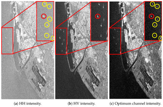
Figure 4.
Optimization results of the C-band quad-polarimetric image acquired over Barcelona (Spain) by Radarsat-2. All figures represent the image intensity in logarithmic scale ranging from −35 to 0 dB. The red circle is used to indicate the ship used to visualize the transects of Figure 5. Yellow circles highlight the rest of vessels present in the scene.
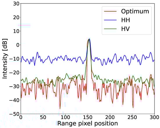
Figure 5.
Azimuth transects through ship shown in magnified region in upper part of Figure 4.
Table 3 presents an estimation of the signal-to-clutter ratio for the same ship. Similar to the previous example with L-band data, the optimized image achieves a higher signal-to-clutter ratio. However, the improvement in this case is less pronounced, with an increase of +6 dB compared to +23 dB in the previous example. In any case, the enhanced contrast between the ship and the sea clutter would improve the automatic detection capabilities of any algorithm.
Table 3.
Signal-to-clutter ratio between the ship highlighted with the red circle in Figure 4 and its surrounding sea clutter for different polarimetric channels.
4.2. Results with Dual-Polarimetric Data
The contrast enhancement processing is now applied to dual-polarimetric SAR data, and the improvements are evaluated across the following different polarization combinations: {HH, VV}, {HH, HV}, and {VV, VH}. In the case of PAZ, which lacks quad-polarimetric capabilities, the acquisition of all three possible polarization combinations can only be achieved on three separate dates (as shown in Table 1). In any case, to ensure a fair comparison among results obtained with different channel combinations, the three images were acquired using the same incidence angle (antenna beam). This way, only eventual changes in sea conditions and the presence of different ships would affect the polarimetric enhancement process. In contrast, since ALOS-1 and Radarsat-2 are quad-polarimetric, all three dual-polarization combinations could be extracted from the same image. Consequently, to test the performance of the method using ALOS-1 and Radarsat-2 dual-pol data, we manually selected two of the four available channels for each of the three cases.
An important aspect of the contrast enhancement technique with dual-pol data is its very fast computation time, since the optimum channel is directly obtained by projecting the complete rank-1 image onto the second eigenvector of the reference patch, as detailed in Section 2.2.
4.2.1. Enhancement Performance with X-Band Dual-Pol Data
Figure 6 shows the results obtained with the dual-pol image of PAZ acquired in the HH and VV channels. As expected, due to the steep incidence angle of the acquisition, the sea response in both co-polar channels is very high, especially in the VV channel, which reduces the contrast between ships and their surrounding background. The rank-1 processing greatly enhances the contrast, as shown in Figure 6c, thereby improving the performance of a ship detector. From this result, we deduce that even though the quad-polarimetric space is not available, the optimization process still clearly cancels the signal from sea areas. Figure 6d shows an azimuth (i.e., vertical) transect of the ship, highlighted by the red rectangle in Figure 6a. As seen in the plots, the VV channel exhibits less contrast (around 15 dB) between the peak (ship pixels) and the lower intensity values (sea area). As expected, HH channel provides a higher signal-to-clutter ratio (around 30 dB) due to a stronger response from the ship (the peak is at 20 dB, compared to 10 dB in VV polarization), while the sea clutter values remain similar (around −10 dB). The optimum channel yields the best results, preserving the peak at a level comparable to HH polarization (around 20 dB) while greatly reducing sea clutter levels to nearly −30 dB.
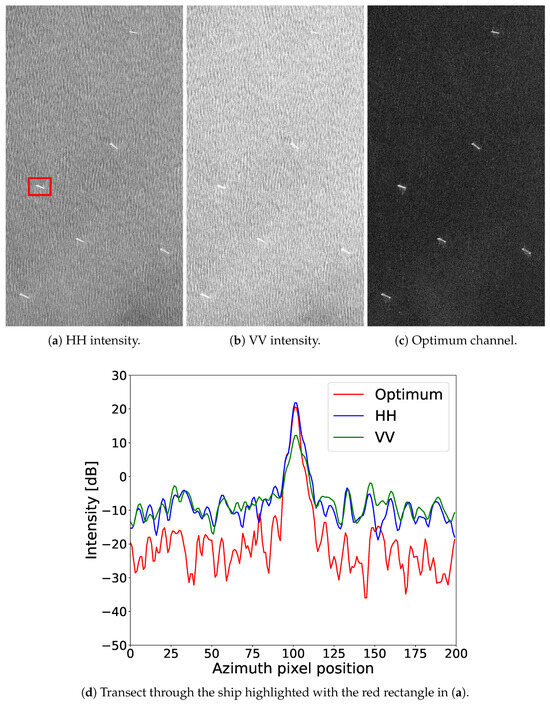
Figure 6.
Optimization results of the dual-polarimetric HH/VV image acquired by PAZ over the coast of Rio Grande (Brazil). Figures (a–c) represent the image intensity in logarithmic scale ranging from −35 to 5 dB. Figure (d) represents a transect through the ship highlighted with the red rectangle in (a).
The second combination of polarizations is {HH, HV}, which corresponds to the two conventional detection channels. Figure 7 shows the optimization results. As in the previous image, HH intensity, which is shown in Figure 7a, exhibits less contrast, i.e., a low signal-to-clutter ratio between ships and surrounding sea areas. The cross-polar HV intensity, depicted in Figure 7b, shows a reduced signal level coming from the sea, thereby improving image contrast. However, note that just by visual inspection, the optimum channel in Figure 7c exhibits again the highest contrast. It is worth noting that, visually, the contrast in the optimum image is similar than to the one obtained in the previous combination. Figure 7d shows an azimuth transect through the ship highlighted by the red rectangle in Figure 7a. As observed, the peak of each plot, corresponding to the ship pixels, is similar across all three channels, with HH intensity being slightly higher at around 11 dB. However, the sea response is significantly lower in the cross-polar channel HV (around −20 dB) compared to HH (−5 dB) and is even further reduced in the optimum channel (around −30 dB).
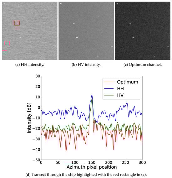
Figure 7.
Optimization results of the dual-polarimetric HH/HV image acquired by PAZ over the coast of Rio Grande (Brazil). Figures (a–c) represent the image intensity in logarithmic scale ranging from −35 to 5 dB. Figure (d) represents a transect through the ship highlighted with the red rectangle in (a).
The last combination of polarimetric channels corresponds to VH and VV. Optimization results are shown in Figure 8. As can be seen in Figure 8a, VV intensity presents a very strong response from the sea, which importantly reduces image contrast. This is the reason why the VV channel is not normally used in vessel detection, as previously stated. The VH channel, which is equivalent to HV in monostatic SAR systems due to reciprocity, exhibits more contrast as shown in Figure 8b. However, the optimized image presents again the highest contrast, with a significantly reduced signal level coming from the sea areas, as shown in Figure 8c.
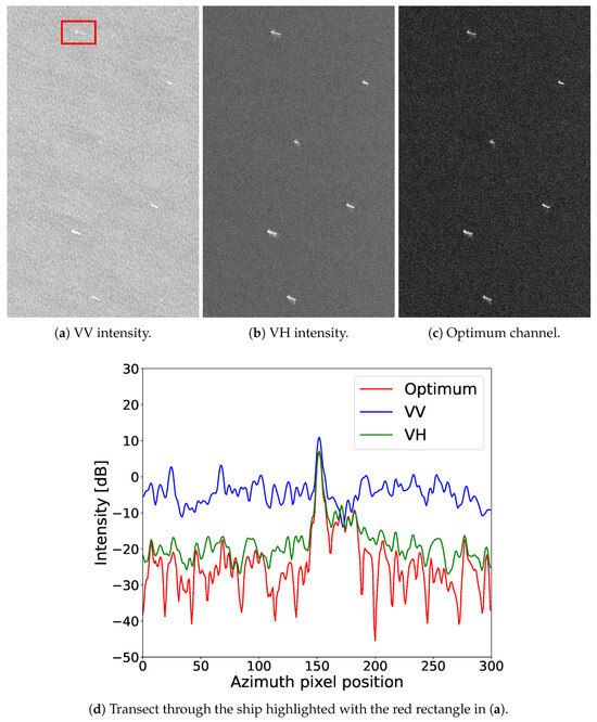
Figure 8.
Optimization results of the dual-polarimetric VH/VV image acquired by PAZ over the coast of Rio Grande (Brazil). Figures (a–c) represent the image intensity in logarithmic scale ranging from −35 to 5 dB. Figure (d) represents a transect through the ship highlighted with the red rectangle in (a).
Numerically, the improvement is quantified for the three combinations of channels by estimating the signal-to-clutter ratio between a ship and the surrounding sea area. Specifically, we use the same ships as those in the transects shown in Figure 6d, Figure 7d, and Figure 8d, highlighted with red rectangles in Figure 6a, Figure 7a, and Figure 8a. The signal-to-clutter ratios are summarized in Table 4. The optimum channels provide consistently the highest signal-to-clutter ratio, regardless of the combination of polarimetric channels.
Table 4.
Signal-to-clutter ratio between a ship and its surrounding sea area after applying the optimization method with different combinations of polarizations using X-band PAZ data.
It is worth noting that, although the three polarimetric images were acquired on different dates, meaning sea conditions might have changed and the selected ships were not the same in all cases, the improvement after applying the optimization remains very similar. In fact, an increase of approximately 10 dB with respect to the best conventional detection channel (either HH or VH/HV) is observed.
4.2.2. Enhancement Performance with C-Band Dual-Pol Data
The quad-pol image gathered by Radarsat-2 over Barcelona (Spain) has been also exploited to evaluate the performance of all combinations of two polarimetric channels corresponding to dual-pol data. Unlike the previous case with PAZ data, the three combinations {HH, VV}, {HH, HV}, and {VV, VH} are available at a single date (see Table 1). To ensure a fair comparison between the different cases, we manually select the same reference sea pixel, which is also the same one we used for the quad-pol optimization of this image analysed in Section 2.1. Additionally, we select the same ship to plot the transects and calculate signal-to-clutter ratios for the three dual-pol cases and the quad-pol case.
Figure 9, Figure 10, and Figure 11 illustrate the results for the polarimetric combinations {HH, VV}, {HH, HV}, and {VV, VH}, respectively. As shown in Figure 9c, Figure 10c, and Figure 11c, the optimized images exhibit enhanced contrast, with a notable reduction in sea clutter. This suppression is particularly pronounced when the cross-polar channel (VH or HV) is employed, as seen in Figure 10c and Figure 11c.
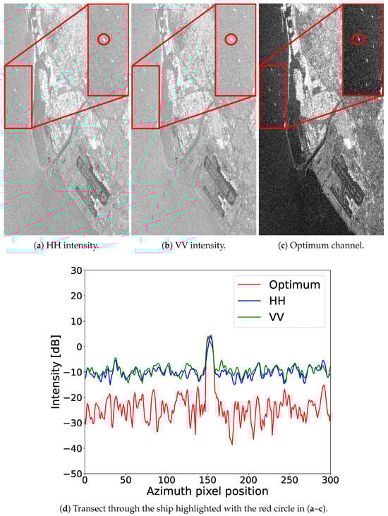
Figure 9.
Optimization results of dual-polarimetric {HH,VV} image acquired by Radarsat-2 over the city of Barcelona (Spain). Figures (a–c) represent the image intensity in logarithmic scale ranging from −35 to 0 dB.
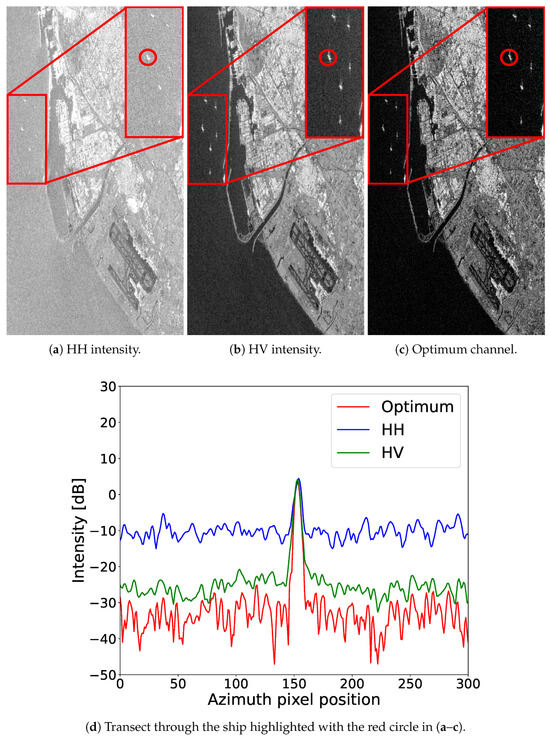
Figure 10.
Optimization results of dual-polarimetric {HH,HV} image acquired by Radarsat-2 over the city of Barcelona (Spain). Figures (a–c) represent the image intensity in logarithmic scale ranging from −35 to 0 dB.
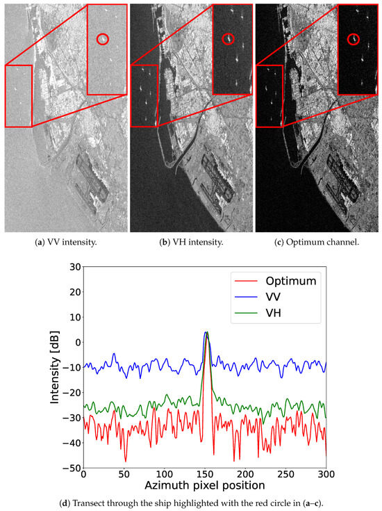
Figure 11.
Optimization results of dual-polarimetric {VV,VH} image acquired by Radarsat-2 over the city of Barcelona (Spain). Figures (a–c) represent the image intensity in logarithmic scale ranging from −35 to 0 dB.
In addition, contrast enhancement is evident in the transects across the same ship, shown in Figure 9d, Figure 10d, and Figure 11d. In all channels (original and optimized), the peak intensity of the transects, corresponding to the ship pixels, remains around 5 dB. However, the sea level is at −10 dB in the co-polar channels (HH and VV) and drops to −25 dB in the cross-polar ones (HV and VH). Comparing the red plots in Figure 9d, Figure 10d, and Figure 11d clearly reveals that sea clutter reduction is more effective when the cross-polar channel is considered. As observed, it decreases to approximately −25 dB for the HH, VV combination and further to around −35 dB for the HH, HV and VV, VH combinations.
In summary, the quantitative improvement with the estimation of the signal-to-clutter ratio between the ship and its surroundings for the three combinations of channels is detailed in Table 5. The optimum channel always provides the highest signal-to-clutter ratio compared to the original channels.
Table 5.
Signal-to-clutter ratio between a ship and its surrounding sea area after applying the contrast enhancement method with different dual-pol combinations of channels using C-band Radarsat-2 data.
As an additional example in the C-band, we apply the contrast optimization technique to a freely available Sentinel-1 dual-polarimetric image acquired over the Strait of Gibraltar in 2018. Polarimetric channels are VV and VH, which correspond to conventional polarizations acquired over land and coastal areas. Optimization results are shown in Figure 12.
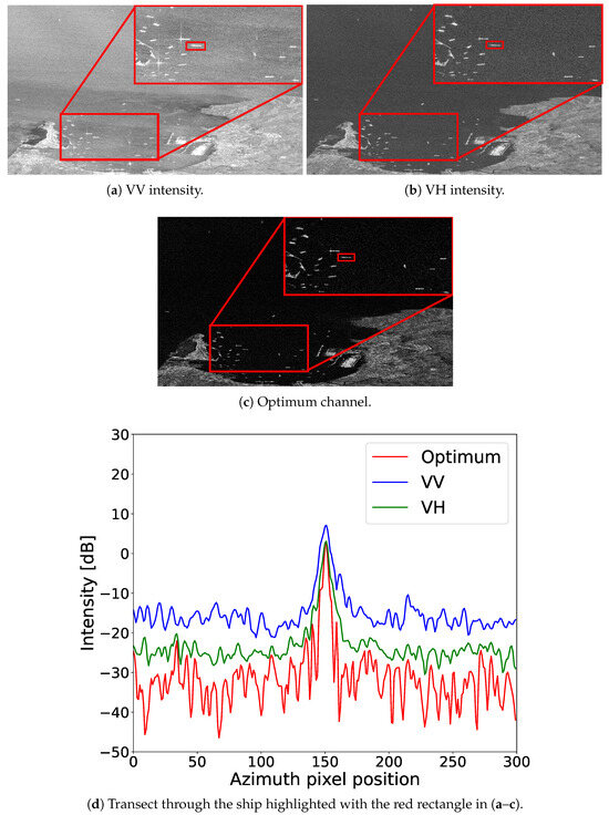
Figure 12.
Optimization results of dual-polarimetric {VV,VH} image acquired by Sentinel-1 over the Strait of Gibraltar. Figures (a–c) represent the image intensity in logarithmic scale ranging from −35 to 0 dB.
As can be seen by comparing Figure 12a,b, VV polarization exhibits, again and as expected, a stronger response of the sea surface compared to VH, leading to reduced contrast between vessels and their surrounding areas. It is clearly observed that contrast is improved in the intensity of the optimized channel, as shown in Figure 12c given the significant reduction in sea clutter level and preservation of signals coming from vessels.
An improvement for the application of automatic detection techniques is further supported by analyzing the transect through the ship shown in Figure 12d. As illustrated, higher intensity values corresponding to the ship pixels are slightly reduced (by approximately 3 dB) in the optimal channel compared to the VV polarization (these values remain very similar to those in the VH polarization). However, the sea clutter level is significantly reduced to around −40 dB in the optimum channel, compared to −15 dB and −25 dB in the VV and VH channels, respectively. More details on the signal-to-clutter ratios are provided in Table 6. As shown, the optimum channel exhibits an improvement of around 9 dB compared to the VH polarization and 13 dB compared to the VV polarization.
Table 6.
Signal-to-clutter ratio between the ship highlighted with the red rectangle in Figure 12 and its surrounding sea clutter for different polarimetric channels.
4.2.3. Enhancement Performance with L-Band Dual-Pol Data
The last set of results follows the same process applied to the Radarsat-2 image in Section 4.2.2, but using the L-band image acquired by ALOS-1 over Tokyo Bay. As in the previous example, we manually select the same sea pixel as a reference for the three dual-pol optimizations. This reference pixel is also the same one used for the quad-pol optimization of this image, detailed in Section 2.1. Additionally, the same vessel is used to plot transects and calculate signal-to-noise ratios, ensuring a fair comparison of the optimization across different polarization inputs.
The results for the three dual-pol combinations—HH, VV, HH, HV, and VV, VH—are presented in Figure 13, Figure 14, and Figure 15, respectively. As evident from these figures, the optimized images consistently exhibit the highest contrast. Furthermore, the transects in Figure 14d and Figure 15d consistently show a greater difference between the peak and the sea signal in the optimized channels (red plots) compared to the original channels (blue and green plots). This difference is particularly pronounced when optimization is applied using the {HH, VV} combination, as shown in Figure 13d. In this case, sea clutter is reduced to below −35 dB (compared to −10 dB in the original channels), while ship intensity increases slightly to approximately 10 dB (compared to around 8 dB in the HH and VV polarizations).
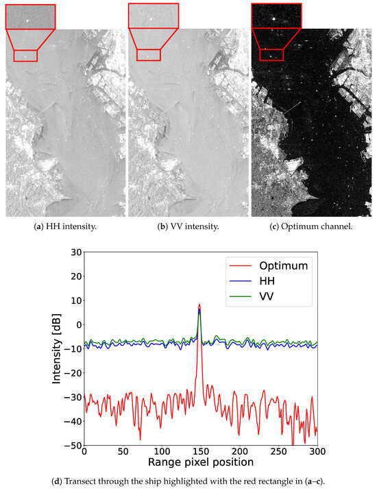
Figure 13.
Optimization results of dual-polarimetric {HH,VV} image acquired by ALOS-1 over Bay of Tokyo (Japan). Figures (a–c) represent image intensity in logarithmic scale ranging from −35 to 0 dB.
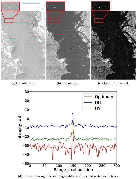
Figure 14.
Optimization results of dual-polarimetric {HH,HV} image acquired by ALOS-1 over Bay of Tokyo (Japan). Figures (a–c) represent image intensity in logarithmic scale ranging from −35 to 0 dB.
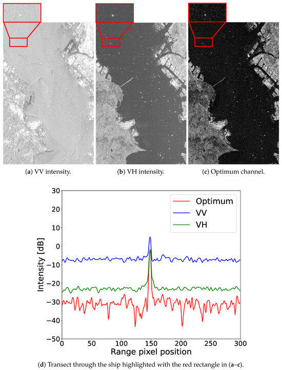
Figure 15.
Optimization results of dual-polarimetric {VV,VH} image acquired by ALOS-1 over Bay of Tokyo (Japan). Figures (a–c) represent image intensity in logarithmic scale ranging from −35 to 0 dB.
Additionally, as illustrated in Figure 14d and Figure 15d, ship intensity in the optimized channels is very similar to that of the cross-polar channels (HV and VH) (around 0 dB). However, the sea intensity level is significantly reduced, further demonstrating that the optimized channels provide the best contrast for ship detection.
Lastly, an estimation of the signal-to-clutter ratio for the three optimization cases is summarized in Table 7. As can be seen, the optimum channel always exhibits the highest values, thus proving again the benefits for ship detection.
Table 7.
Signal-to-clutter ratio between a ship and its surrounding sea area after applying the contrast enhancement method with different dual-pol combinations of channels using L-band ALOS-1 data.
5. Discussion
A contrast enhancement technique [31] based on polarimetric orthogonality has been applied as a pre-processing step to improve automatic ship detection with SAR images. The enhancement performance has been evaluated with different SAR sensors working in the L-, C-, and X-bands. The formulation, originally proposed for quad-polarimetric data, has been adapted to the dual-pol case and has been shown to provide improved results also for dual-pol images by enhancing the image contrast for automatic detection purposes. As shown, the polarimetric processing applied always improves the signal-to-clutter ratio between the ships and the surrounding sea clutter compared to conventional detection channels (HH or HV), hence easing the application of any automatic ship detector.
It is worth mentioning that the application of contrast enhancement techniques to SAR data to improve ship detection has been intensively studied in previous works. On the one hand, methods based on spectral analysis exploit the properties of the spectrum of SLC SAR images. The fundamental idea of these methods is that vessels and their surrounding sea areas present different spectral properties. Therefore, portions of a whole image spectrum (denoted as a sub-spectrum) are progressively extracted and processed. The goal of spectral methods is then to cancel undesired contributions coming from the sea areas, while simultaneously preserving ship spectral information, hence increasing the ship-over-sea contrast on the original image domain. A review of such methods can be found in the following references [35,36,37].
On the other hand, a second group of contrast enhancement algorithms for ship detection is purely based on polarimetric optimizations. As the name suggests, this second group of detectors involves a numerical optimization of the polarimetric information. A first approach was originally proposed in [38] with the development of a Polarimetric Matched Filter (PMF), the goal of which was to suppress sea clutter by weighting the polarimetric target vector using the information of targets (i.e., vessels) and the sea clutter. The Optimal Polarimetric Detector (OPD) is based on maximizing a likelihood ratio test (LRT) between the quadratic forms of the polarimetric covariance matrices of ships and clutter [25,39]. Then, a variety of more sophisticated OPCE (Optimal Polarimetric Contrast Enhancement) methods were raised to improve ship detection performance [40,41,42] for both the coherent and incoherent cases. Also, the Polarimetric Whitening Filter (PWF) and its variants [43,44,45], which exploit polarimetric information to minimize statistical image data variations due to speckle, are widely used to improve contrast between ships and sea clutter. More recent methods for contrast optimization include the Polarimetric Notch Filter (PNC) [23,30,46], which uses a physical interpretation of the sea clutter and minimizes its response.
The technique applied in this work should be categorized within the second group of contrast enhancers, since it is based on exploiting the available polarimetric space provided by either two or four polarimetric channels. However, it presents important differences compared to traditional contrast optimization techniques using polarimetry. The first key difference is that its design does not depend on the final performance of the detector because it is just a pre-processing step to be carried out before any detector is applied. In this sense, its applicability is very general, as it helps any detector and is not conditioned by later processing stages. Another major difference is that it is not really an optimization from the numerical point of view, since the solution it provides is completely analytical for both the dual- and quad-pol cases. In fact, its computation is significantly faster than other contrast optimizers. In addition, it only requires selecting a reference pixel (or patch) from the background to be cancelled, with the consequence that knowledge about the scattering properties of ships is not required.
6. Conclusions
This work has demonstrated that the rank-1 polarimetric technique proposed in [31] consistently provides enhanced contrast, making the output images more suitable for the application of any automatic vessel detection method.
The results show that sea clutter is significantly reduced across all polarization combinations, whether dual- or quad-pol data are employed. Furthermore, it has been shown that the technique delivers improved performance across all L-, C-, and X-bands.
As future work, we plan to conduct a more detailed analysis focusing on images acquired outside the nominal incidence angles, often referred to as out-of-performance images. These images correspond to scenarios where the SAR system operates outside its optimal design parameters, as with a very shallow incidence angle, resulting in increased backscatter from the sea surface. Such images are particularly important from an operational perspective for ship detection, as customers often need to process the first available image, which may fall into this out-of-performance category. In addition, the behaviour of the polarimetric contrast optimization in the presence of ambiguities also deserves to be studied in the future. Ambiguities are an aliasing effect coming from the sampling of the scene which causes the same target to appear in different image positions. Because backscattered signals coming from the sea surface are much lower than those coming from coastal urban areas and vessels, ambiguities are especially visible in sea areas. Finally, we aim to evaluate the contrast enhancement approach for land targets to further assess its applicability and effectiveness in other scenarios.
Author Contributions
Conceptualization and methodology, A.M.-Q. and J.M.L.-S.; software, A.M.-Q.; validation, A.M.-Q.; formal analysis, A.M.-Q.; investigation, A.M.-Q.; writing—original draft preparation, A.M.-Q.; writing—review and editing, J.M.L.-S.; visualization, A.M.-Q.; supervision, J.M.L.-S. All authors have read and agreed to the published version of the manuscript.
Funding
This research was funded by the Spanish Ministry of Science and Innovation (State Agency of Research, AEI) and the European Funds for Regional Development under grant number PID2020-117303GB-C22/AEI/10.13039/501100011033.
Institutional Review Board Statement
Not applicable.
Informed Consent Statement
Not applicable.
Data Availability Statement
The datasets presented in this article are not readily available because they are provided by spatial agencies only for scientific purposes upon request.
Acknowledgments
The ALOS-1 image ©JAXA/METI ALOS PALSAR L1.1 2008 was downloaded from the Alaska SAR Facility (accessed through ASF DAAC 1 November 2024). RADARSAT-2 Data and Products © MacDonald, Dettwiler and Associates Ltd. (MDA) (2011)—All Rights Reserved. RADARSAT is an official trademark of the Canadian Space Agency (CSA). The Radarsat-2 image was provided by the MDA and CSA within the framework of project SOAR-EU 6779. All PAZ images were kindly provided by Hisdesat Strategic Services.
Conflicts of Interest
The authors declare no conflict of interest.
References
- Ao, W.; Xu, F.; Li, Y.; Wang, H. Detection and Discrimination of Ship Targets in Complex Background From Spaceborne ALOS-2 SAR Images. IEEE J. Sel. Top. Appl. Earth Obs. Remote Sens. 2018, 11, 536–550. [Google Scholar] [CrossRef]
- Brusch, S.; Lehner, S.; Fritz, T.; Soccorsi, M.; Soloviev, A.; van Schie, B. Ship Surveillance with TerraSAR-X. IEEE Trans. Geosci. Remote Sens. 2011, 49, 1092–1103. [Google Scholar] [CrossRef]
- Dai, H.; Du, L.; Wang, Y.; Wang, Z. A Modified CFAR Algorithm Based on Object Proposals for Ship Target Detection in SAR Images. IEEE Geosci. Remote Sens. Lett. 2016, 13, 1925–1929. [Google Scholar] [CrossRef]
- Leng, X.; Ji, K.; Yang, K.; Zou, H. A Bilateral CFAR Algorithm for Ship Detection in SAR Images. IEEE Geosci. Remote Sens. Lett. 2015, 12, 1536–1540. [Google Scholar] [CrossRef]
- Wang, C.; Guo, B.; Song, J.; He, F.; Li, C. A Novel CFAR-Based Ship Detection Method Using Range-Compressed Data for Spaceborne SAR System. IEEE Trans. Geosci. Remote Sens. 2024, 62, 1–15. [Google Scholar] [CrossRef]
- Zhang, L.; Zhang, Z.; Lu, S.; Xiang, D.; Su, Y. Fast Superpixel-Based Non-Window CFAR Ship Detector for SAR Imagery. Remote Sens. 2022, 14, 2092. [Google Scholar] [CrossRef]
- Li, Y.; Wang, Z.; Chen, H.; Li, Y. A Density Clustering-Based CFAR Algorithm for Ship Detection in SAR Images. IEEE Geosci. Remote Sens. Lett. 2024, 21, 1–5. [Google Scholar] [CrossRef]
- Li, H.C.; Krylov, V.A.; Fan, P.Z.; Zerubia, J.; Emery, W.J. Unsupervised Learning of Generalized Gamma Mixture Model with Application in Statistical Modeling of High-Resolution SAR Images. IEEE Trans. Geosci. Remote Sens. 2016, 54, 2153–2170. [Google Scholar] [CrossRef]
- Zhu, X.X.; Montazeri, S.; Ali, M.; Hua, Y.; Wang, Y.; Mou, L.; Shi, Y.; Xu, F.; Bamler, R. Deep Learning Meets SAR: Concepts, models, pitfalls, and perspectives. IEEE Geosci. Remote Sens. Mag. 2021, 9, 143–172. [Google Scholar] [CrossRef]
- Li, J.; Xu, C.; Su, H.; Gao, L.; Wang, T. Deep Learning for SAR Ship Detection: Past, Present and Future. Remote Sens. 2022, 14, 2712. [Google Scholar] [CrossRef]
- Huang, Z.; Liu, Y.; Yao, X.; Ren, J.; Han, J. Uncertainty Exploration: Toward Explainable SAR Target Detection. IEEE Trans. Geosci. Remote Sens. 2023, 61, 1–14. [Google Scholar] [CrossRef]
- Zhang, C.; Zhang, X.; Zhang, J.; Gao, G.; Dai, Y.; Liu, G.; Jia, Y.; Wang, X.; Zhang, Y.; Bao, M. Evaluation and Improvement of Generalization Performance of SAR Ship Recognition Algorithms. IEEE J. Sel. Top. Appl. Earth Obs. Remote Sens. 2022, 15, 9311–9326. [Google Scholar] [CrossRef]
- Deng, Z.; Sun, H.; Zhou, S.; Zhao, J. Learning Deep Ship Detector in SAR Images From Scratch. IEEE Trans. Geosci. Remote Sens. 2019, 57, 4021–4039. [Google Scholar] [CrossRef]
- Li, J.; Chen, J.; Cheng, P.; Yu, Z.; Yu, L.; Chi, C. A Survey on Deep-Learning-Based Real-Time SAR Ship Detection. IEEE J. Sel. Top. Appl. Earth Obs. Remote Sens. 2023, 16, 3218–3247. [Google Scholar] [CrossRef]
- Alexandre, C.; Devillers, R.; Mouillot, D.; Seguin, R.; Catry, T. Ship Detection with SAR C-Band Satellite Images: A Systematic Review. IEEE J. Sel. Top. Appl. Earth Obs. Remote Sens. 2024, 17, 14353–14367. [Google Scholar] [CrossRef]
- Gierull, C.H.; Rashid, M. Indicating Ambiguous False Positives to Improve Wide-Area SAR Vessel Detection. IEEE Trans. Geosci. Remote Sens. 2024, 62, 1–13. [Google Scholar] [CrossRef]
- Wahl, D.; Eichel, P.; Ghiglia, D.; Jakowatz, C. Phase gradient autofocus-a robust tool for high resolution SAR phase correction. IEEE Trans. Aerosp. Electron. Syst. 1994, 30, 827–835. [Google Scholar] [CrossRef]
- Xi, L.; Guosui, L.; Ni, J. Autofocusing of ISAR images based on entropy minimization. IEEE Trans. Aerosp. Electron. Syst. 1999, 35, 1240–1252. [Google Scholar] [CrossRef]
- Salvetti, F.; Martorella, M.; Giusti, E.; Staglianò, D. Multiview Three-Dimensional Interferometric Inverse Synthetic Aperture Radar. IEEE Trans. Aerosp. Electron. Syst. 2019, 55, 718–733. [Google Scholar] [CrossRef]
- Kumar, A.; Giusti, E.; Mancuso, F.; Ghio, S.; Lupidi, A.; Martorella, M. Three-Dimensional Polarimetric InISAR Imaging of Non-Cooperative Targets. IEEE Trans. Comput. Imaging 2023, 9, 210–223. [Google Scholar] [CrossRef]
- Touzi, R.; Raney, R.; Charbonneau, F. On the use of permanent symmetric scatterers for ship characterization. IEEE Trans. Geosci. Remote Sens. 2004, 42, 2039–2045. [Google Scholar] [CrossRef]
- Fan, W.; Zhou, F.; Tao, M.; Bai, X.; Shi, X.; Xu, H. An Automatic Ship Detection Method for PolSAR Data Based on K-Wishart Distribution. IEEE J. Sel. Top. Appl. Earth Obs. Remote Sens. 2017, 10, 2725–2737. [Google Scholar] [CrossRef]
- Marino, A. A Notch Filter for Ship Detection with Polarimetric SAR Data. IEEE J. Sel. Top. Appl. Earth Obs. Remote Sens. 2013, 6, 1219–1232. [Google Scholar] [CrossRef]
- Zhang, T.; Ji, J.; Li, X.; Yu, W.; Xiong, H. Ship Detection From PolSAR Imagery Using the Complete Polarimetric Covariance Difference Matrix. IEEE Trans. Geosci. Remote Sens. 2019, 57, 2824–2839. [Google Scholar] [CrossRef]
- Hajnsek, I.; Desnos, Y.L. Polarimetric Synthetic Aperture Radar: Principles and Application; Springer: Berlin/Heidelberg, Germany, 2009. [Google Scholar]
- Zhang, T.; Quan, S.; Yang, Z.; Guo, W.; Zhang, Z.; Gan, H. A Two-Stage Method for Ship Detection Using PolSAR Image. IEEE Trans. Geosci. Remote Sens. 2022, 60, 1–18. [Google Scholar] [CrossRef]
- Velotto, D.; Nunziata, F.; Migliaccio, M.; Lehner, S. Dual-Polarimetric TerraSAR-X SAR Data for Target at Sea Observation. IEEE Geosci. Remote Sens. Lett. 2013, 10, 1114–1118. [Google Scholar] [CrossRef]
- Shirvany, R.; Chabert, M.; Tourneret, J.Y. Ship and Oil-Spill Detection Using the Degree of Polarization in Linear and Hybrid/Compact Dual-Pol SAR. IEEE J. Sel. Top. Appl. Earth Obs. Remote Sens. 2012, 5, 885–892. [Google Scholar] [CrossRef]
- Mitsunobu Sugimoto, K.O.; Nakamura, Y. On the novel use of model-based decomposition in SAR polarimetry for target detection on the sea. Remote Sens. Lett. 2013, 4, 843–852. [Google Scholar] [CrossRef]
- Marino, A.; Hajnsek, I. Statistical Tests for a Ship Detector Based on the Polarimetric Notch Filter. IEEE Trans. Geosci. Remote Sens. 2015, 53, 4578–4595. [Google Scholar] [CrossRef]
- Cloude, S.R. Target Detection Using Rank-1 Polarimetric Processing. IEEE Geosci. Remote Sens. Lett. 2021, 18, 717–720. [Google Scholar] [CrossRef]
- Lee, J.S.; Pottier, E. Polarimetric Radar Imaging: From Basics to Applications; CRC Press: Boca Raton, FL, USA, 2009. [Google Scholar]
- Touzi, R.; Vachon, P.W.; Wolfe, J. Requirement on Antenna Cross-Polarization Isolation for the Operational Use of C-Band SAR Constellations in Maritime Surveillance. IEEE Geosci. Remote Sens. Lett. 2010, 7, 861–865. [Google Scholar] [CrossRef]
- Touzi, R.; Hurley, J.; Vachon, P.W. Optimization of the Degree of Polarization for Enhanced Ship Detection Using Polarimetric RADARSAT-2. IEEE Trans. Geosci. Remote Sens. 2015, 53, 5403–5424. [Google Scholar] [CrossRef]
- Souyris, J.C.; Henry, C.; Adragna, F. On the use of complex SAR image spectral analysis for target detection: Assessment of polarimetry. IEEE Trans. Geosci. Remote Sens. 2003, 41, 2725–2734. [Google Scholar] [CrossRef]
- Brekke, C.; Anfinsen, S.N.; Larsen, Y. Subband Extraction Strategies in Ship Detection with the Subaperture Cross-Correlation Magnitude. IEEE Geosci. Remote Sens. Lett. 2013, 10, 786–790. [Google Scholar] [CrossRef]
- Marino, A.; Sanjuan-Ferrer, M.J.; Hajnsek, I.; Ouchi, K. Ship Detection with Spectral Analysis of Synthetic Aperture Radar: A Comparison of New and Well-Known Algorithms. Remote Sens. 2015, 7, 5416–5439. [Google Scholar] [CrossRef]
- Boerner, W.M.; Kostinski, A. On the concept of the polarimetric matched filter in high resolution radar imaging. In Proceedings of the 1988 IEEE AP-S. International Symposium, Antennas and Propagation, Syracuse, NY, USA, 6–10 June 1988; Volume 2, pp. 533–536. [Google Scholar] [CrossRef]
- Novak, L.; Sechtin, M.; Cardullo, M. Studies of target detection algorithms that use polarimetric radar data. IEEE Trans. Aerosp. Electron. Syst. 1989, 25, 150–165. [Google Scholar] [CrossRef]
- Yang, J.; Yamaguchi, Y.; Boerner, W.M.; Lin, S. Numerical methods for solving the optimal problem of contrast enhancement. IEEE Trans. Geosci. Remote Sens. 2000, 38, 965–971. [Google Scholar] [CrossRef]
- Liu, C.; Vachon, P.W.; Geling, G.W. Improved ship detection with airborne polarimetric SAR data. Can. J. Remote Sens. 2005, 31, 122–131. [Google Scholar] [CrossRef]
- Yang, D.; Du, L.; Liu, H.; Ni, W. Novel Polarimetric Contrast Enhancement Method Based on Minimal Clutter to Signal Ratio Subspace. IEEE Trans. Geosci. Remote Sens. 2019, 57, 8570–8583. [Google Scholar] [CrossRef]
- Novak, L.; Burl, M. Optimal speckle reduction in polarimetric SAR imagery. IEEE Trans. Aerosp. Electron. Syst. 1990, 26, 293–305. [Google Scholar] [CrossRef]
- Lopes, A.; Sery, F. Optimal speckle reduction for the product model in multilook polarimetric SAR imagery and the Wishart distribution. IEEE Trans. Geosci. Remote Sens. 1997, 35, 632–647. [Google Scholar] [CrossRef]
- Liu, T.; Zhang, J.; Gao, G.; Yang, J.; Marino, A. CFAR Ship Detection in Polarimetric Synthetic Aperture Radar Images Based on Whitening Filter. IEEE Trans. Geosci. Remote Sens. 2020, 58, 58–81. [Google Scholar] [CrossRef]
- Marino, A.; Sugimoto, M.; Ouchi, K.; Hajnsek, I. Validating a Notch Filter for Detection of Targets at Sea with ALOS-PALSAR Data: Tokyo Bay. IEEE J. Sel. Top. Appl. Earth Obs. Remote Sens. 2014, 7, 4907–4918. [Google Scholar] [CrossRef]
Disclaimer/Publisher’s Note: The statements, opinions and data contained in all publications are solely those of the individual author(s) and contributor(s) and not of MDPI and/or the editor(s). MDPI and/or the editor(s) disclaim responsibility for any injury to people or property resulting from any ideas, methods, instructions or products referred to in the content. |
© 2025 by the authors. Licensee MDPI, Basel, Switzerland. This article is an open access article distributed under the terms and conditions of the Creative Commons Attribution (CC BY) license (https://creativecommons.org/licenses/by/4.0/).