Abstract
The widespread presence of security patterns in modern anti-forgery systems has given rise to an urgent need for reliable smartphone authentication. However, persistent recognition inaccuracies occur because of the inherent degradation of patterns during smartphone capture. These acquisition-related artifacts are manifested as both spectral distortions in high-frequency components and structural corruption in the spatial domain, which essentially limit current verification systems. This paper addresses these two challenges through four key innovative aspects: (1) It introduces a chromatic-adaptive coupled oscillation mechanism to reduce noise. (2) It develops a DFT-domain processing pipeline. This pipeline includes micro-feature degradation modeling to detect high-frequency pattern elements and directional energy concentration for characterizing motion blur. (3) It utilizes complementary spatial-domain constraints. These involve brightness variation for local consistency and edge gradients for local sharpness, which are jointly optimized by combining maximum a posteriori estimation and maximum likelihood estimation. (4) It proposes an adaptive graph-based partitioning strategy. This strategy enables spatially variant kernel estimation, while maintaining computational efficiency. Experimental results showed that our method achieved excellent performance in terms of deblurring effectiveness, runtime, and recognition accuracy. This achievement enables near real-time processing on smartphones, without sacrificing restoration quality, even under difficult blurring conditions.
1. Introduction
Anti-forgery techniques are a range of measures designed to protect businesses and consumers from unauthorized counterfeit products [1]. With the increasing sophistication of high-quality counterfeiting techniques, digital image-based anti-counterfeiting techniques have attracted widespread attention. Quick response (QR) codes have emerged as a particularly effective medium, leveraging their high-density data encoding capacity and machine-readable efficiency. Recent advancements have expanded QR code functionality through multiple security-enhanced implementations: physically unclonable functions (PUF) [2,3], watermarks [4], copy detection patterns (CDP) [5], and patch-wise color patterns. Figure 1 illustrates representative implementations of security patterns. However, in the process of capturing patterns, factors such as shooting habits, equipment, and environmental conditions often result in blurred images. This operational reality necessitates robust deblurring frameworks to ensure reliability. Current research developments in image deblurring can be broadly classified into the following categories:
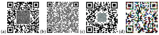
Figure 1.
Security patterns. (a) PUF; (b) watermark; (c) CDP; (d) patch-wise color pattern.
(1) Model-based methods: Pan et al. [6] proposed an L0 regularization method specifically for the text image deblurring problem. This method preserves the intensity and gradient information of the image by minimizing the L0 parameter and is particularly suitable for text images with clear edges. However, L0 regularization can lead to an increase in computational complexity. Anwar et al. [7] proposed an image deblurring method with class-specific prior knowledge for different types of content. This method provides accurate results for specific image classes but requires a large amount of annotation data and in-depth knowledge of each class. Moreover, it may be ineffective for images with mixed or unspecified classes. Bai et al. [8] proposed a single-image blind deblurring method. This method uses a multi-scale latent structure prior to help estimate the blur kernel and recover the image. It is good at dealing with complex blur situations. However, the method is complicated and requires many parameter adjustments. Bai et al. [9] required only a single blur image to construct a graph model that characterizes the relationship between image content and the blur process, without additional information. This method can handle complex structures and blur situations. Nevertheless, it is sensitive to noise and computationally complex. Wen et al. [10] proposed a simple blind deblurring method based on the local minimum pixel intensity prior. This method uses the local minimum pixel intensity to estimate the blur kernel. It is easy to implement and provides kernel estimation. However, the effect may be poor with complex scenes or for specific blur types, and it relies on the previous accuracy and universality. Zhang et al. [11] explored the iterative optimization process and put forward a pixel screening method. This method is designed to correct intermediate images and filter out bad pixels, thereby facilitating more precise kernel estimation. Alexander et al. [12] put forward a semi-blind image deblurring problem. By applying the proposed iterative schemes, they aimed to recover a clear image from a noisy and blurred one. Their motion deblurring schemes can compete with modern non-blind methods, despite using less information. Moreover, the proposed schemes are also applicable to inverting non-linear filters and can rival state-of-the-art black-box defiltering methods. Shao et al. [13] rethought the regularization term in the image blind deblurring problem and proposed a more realistic regularization method, to provide a more accurate model for describing the characteristics of an image. However, their new regularization term may require a complex optimization strategy, which increases the computational complexity and time cost. Cai et al. [14] proposed an a priori constraint that is founded on maximizing local high-frequency wavelet coefficients. This constraint is incorporated into a graph-based blind deblurring model. To handle the non-convex and nonlinear model, an alternating iteration method is utilized, which is combined with a simple thresholding technique. Huang et al. [15] put forward a differential Lorentzian point spread function model. This model has the ability to represent the line spread function of a real image as a series of Lorentzian functions with variable pulse widths and combinations of their differential functions. After that, an algorithm for estimating the model parameters, which is based on the improved zeroing filter, was presented.
(2) Deep-learning-based methods: Ren et al. [16] proposed a spatially varying neural network, which is composed of a recurrent neural network (RNN) and three deep convolutional neural networks (CNNs). The RNN functions as a deconvolution operator on the feature maps derived from the input image. Two CNNs are utilized for feature extraction and for generating pixel-level weights for the spatially varying RNN. During the image reconstruction phase, a CNN is employed to estimate the final deblurred image. Bono et al. [17] noted that the basic RNN unit has difficulty capturing long-term temporal dependencies, due to the vanishing gradient problem. Both Long Short-Term Memory (LSTM) and the Gated Recurrent Unit (GRU) are variants of the simple recurrent unit and can effectively address time-related issues. Ma et al. [18] proposed a deblurring network with defocus map estimation as an auxiliary task. This network improves the overall processing capability through dual-task learning. However, the extra task increases the computational burden and may affect the deblurring results if the estimation of the auxiliary task is inaccurate. Que et al. [19] proposed a lightweight dynamic deblurring solution for IoT smart cameras that is suitable for resource-constrained environments. Nevertheless, it may require further optimization in high-complexity scenarios. Wang et al. [20] proposed a special GAN architecture with multiple residual learning modules. This architecture effectively handles multiple blur situations by introducing residual structures. However, it requires a large amount of training data for optimization and may not be effective under extreme blur conditions. Li et al. [21] proposed an image deblurring method using image blur, which enables the network to focus on the hard-to-recover high-frequency details and performs well under certain blur types, but requires specific tuning for different blur types. Sharif et al. [22] proposed a deblurring method for single-frame images in low-light conditions and that solves the blur problem at night or in low-light environments, but further optimization is needed when dealing with dynamic blur or complex scenes. Mao et al. [23] introduced a highly efficient single-image blind deblurring technique based on deep idempotent networks. This technique maintains processing stability through idempotent constraints, does not require other auxiliary information, and has strong generalization ability. However, it has high complexity and requires careful tuning of hyperparameters. Liang et al. [24] seamlessly encoded both spatial details and contextual information. Their approach decouples the intricate deblurring task into two distinct subtasks: a primary feature encoder and a contextual encoder. Subsequently, the combined outputs of these encoders are merged by a decoder to reconstruct the sharp target image. Quan et al. [25] utilized a pixel-wise Gaussian kernel mixture model to precisely and concisely parameterize the spatially-varying defocus point spread functions. Feng et al. [26] made use of alternating iterations of shrinkage thresholds, which included updating blurring kernels and images. Moreover, they put forward a learnable blur kernel proximal mapping module to enhance the accuracy of the blur kernel reconstruction. This module also integrates an attention mechanism to adaptively learn the significance of prior information. Zhuang et al. [27] put forward a multi-domain adaptive deblurring network consisting of two modules. One is the domain adaptation module, which makes use of domain-invariant features to ensure the stable performance of the network across multiple domains. The other is the meta deblurring module, which utilizes the auxiliary branch to improve the deblurring capacity.
(3) Security pattern deblurring: Given that methods formulated for natural images typically do not exhibit good generalization to patterns, researchers have devised several effective priors grounded in the characteristics of QR codes. For example, Shi et al. [28] put forward a line search method grounded in binary property metrics with the aim of reducing the time consumed in searching for the optimal blur kernel. Nevertheless, this approach is solely applicable to linear blur in conveyor belt scenarios, and its applicability is severely restricted. Rioux et al. [29] proposed a barcode blind deblurring method based on Kullback–Leibler scattering. The method recovers the code by minimizing the KL scattering between the blurred barcode and the clear barcode, making it particularly suitable for motion blur. However, it may require significant computational resources, and its performance may be degraded when dealing with low-quality or extremely blurred barcodes. Chen et al. [30] introduced a fast QR code recovery method for blur caused by inaccurate focusing. The method incorporates edge prior information into the code sensing stage, resulting in faster recovery and improved quality. However, the accuracy is dependent on the prior information and parameter settings. Improper settings may negatively impact the recovery effect, particularly in cases of complex blurring or noise interference. Chen et al. [31] presented a method that directly estimates image sharpness based on image gradient features. This method can halt multi-scale iteration estimation at a scale enabling QR code recognition. However, in practical applications where the scene changes frequently, its implementation proves to be challenging. Li et al. [32] extracted the key features of the blurred QR codes, binarized them using an improved adaptive thresholding method, and finally decoded them. This method is effective in solving the blur caused by rapid camera or object movement, with a high recognition rate and computational efficiency able to meet the demands of real-time applications. However, further optimization may be necessary when dealing with complex blurring patterns. Zheng et al. [33] proposed a blind deblurring method for anti-counterfeit 2D codes that combines intensity and gradient priors. This method is specifically designed for security QR codes with specific localization patterns, and it can accurately recover blurred QR codes by considering local intensity and gradient information. Xu et al. [34] proposed an approach that capitalizes on local maximum and minimum intensity priors. This algorithm adaptively performs binarization of the intensity within the maximum a posteriori framework, resulting in a significant enhancement in computational efficiency. Eventually, latent image estimation and kernel estimation are alternately solved within the framework until convergence is achieved.
Although model-based deblurring methods show advantages in improving the recovery of image details and the sharpness of edges, their practical application is still restricted by several intrinsic drawbacks. These drawbacks include high computational complexity, sensitivity to noise, and the need for demanding parameter optimization. Deep-learning-based methods, even though they perform excellently in dealing with various types of blur and reconstructing fine image details, also face their own problems. These problems involve heavy reliance on a large amount of training data, high computational costs, limited generalization ability, and subpar performance under extreme blur situations. In the particular field of security pattern restoration, the existing deblurring techniques have been effective in enhancing practical robustness. However, they still have crucial limitations when dealing with severely damaged patterns or operating under resource limitations. Significantly, color security patterns bring both opportunities and challenges. Compared with traditional grayscale patterns, color security patterns have many advantages in aspects such as tamper resistance, fraud prevention, information density, visual attractiveness, and authentication reliability. But at the same time, they make the tasks of removing blur and restoring sharpness more complex.
To address these various challenges, this paper puts forward a comprehensive framework for security pattern restoration through fundamental theoretical innovations, as depicted in Figure 2. Firstly, we present chromatic-adaptive coupled oscillation (CACO), a physics-inspired enhancement technique. This technique establishes channel-specific nonlinear transformations and cross-channel dynamic coupling. It can achieve excellent noise suppression, while maintaining color fidelity and structural details, without the need for training data. Secondly, we propose micro-feature degradation and directional energy concentration (MDDEC), a novel blur detection algorithm. This algorithm combines spectral whitening with adaptive morphological filtering and hierarchical classification of fused global-directional features, showing high accuracy in blur-type discrimination under various imaging conditions. Thirdly, we introduce an optimized blind deblurring framework with graph-guided partition for localized kernel estimation. Regarding defocus blur, the mathematical basis is derived from unifying minimum brightness difference (MBD) and edge gradient (EG) priors within a hybrid energy functional. This enables closed-form FFT solutions that converge more rapidly than iterative alternatives. For motion blur, we prove that the MBD–EG–DEC feature triplet forms a complete basis for kernel estimation, and the second-order moments of the YCbCr luminance channel provide sufficient information for coarse-to-fine restoration. Our main contributions are as follows:
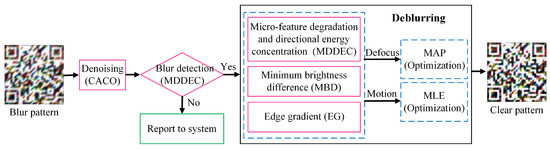
Figure 2.
The flowchart of the proposed method.
- The preprocessing technique employed is denoising with chromatic-adaptive coupled oscillation (CACO). This technique augments the contrast and details, thereby enhancing the overall quality of patterns. Micro-feature degradation and directional energy concentration (MDDEC) is introduced for blur detection, enabling the quantitative detection of the degree of blurring of patterns.
- Extra priors, a minimum brightness difference (MBD) prior and an edge gradient (EG) prior, are integrated as constraints into maximum a posteriori (MAP) and maximum likelihood estimation (MLE) frameworks. These pattern-specific priors significantly enhance the recovery of structure and details.
- By partitioning the pattern into several sub-regions and employing graphical guidance to group these sub-regions, the problem of pattern content variability and non-uniform blur has been effectively addressed.
- The experimental results demonstrate the robustness of the proposed method and a significant reduction in runtime.
The paper is organized as follows: An efficient blur detection method for security patterns is proposed in Section 2. A novel blind deblurring algorithm is developed in detail in Section 3. Section 4 gives the experimental results and a discussion. Finally, the conclusions and future improvements are presented in Section 5.
2. Blur Detection of Security Patterns
2.1. Blur Degrading
The blur degrading process of security patterns can be conceptualized as the convolution of a clear pattern with a kernel function, accompanied by additive noise that is analogous to white Gaussian noise. Under the assumption that the blur is uniform and spatially invariant, the mathematical model of an individual blur pattern can be expressed as follows:
where B, k, ⊗, C, and n represent the blur pattern, blur kernel, convolution operation, clear pattern, and additive noise, respectively.
Progressive blur degradation simulation of security patterns is shown in Figure 3. Blur patterns can be deblurred by blur-kernel-based deconvolution, while minimizing the effect of noise on the deconvolution process. However, since the blur kernel is usually unknown, deconvolution becomes an ill-posed problem with multiple possible solutions. Therefore, it is usually necessary to perform blur estimation beforehand by utilizing the information and features of the blur pattern. The potential blur kernels are identified, and the pattern is then deblurred through deconvolution. The efficacy of the deblurring process is contingent upon the precision of the blur kernel estimation and the selected deblurring methodology. Two common types of blur in image processing are defocus blur and motion blur. The essential difference between these two types of blur lies in the difference in their blur kernel functions. In order to investigate the blur parameters more accurately, it is necessary to categorize the different types of image blur and use corresponding processing methods according to the different types. To facilitate this classification and subsequent processing, we initially formalize the kernel functions associated with these two primary types of blur:
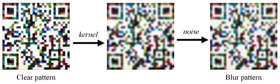
Figure 3.
Progressive blur degradation simulation of security patterns.
(1) The phenomenon of defocus blur is typically attributed to inaccurate focusing or a disparity in depth of field within the scene during the capturing process. With regard to security patterns, the primary cause of defocus blur is typically an inaccurate focus. Its blur kernel function can be expressed as follows:
where R represents the radius of the defocus blur spot.
(2) Motion blur is caused by the relative displacement of the camera with respect to the capturing target during the exposure time. In the study of security patterns, global motion blur due to the shaking of the capturing equipment is the most prevalent cause. Since the exposure time is usually short, the relative motion of the camera and the pattern can be approximated as a uniform linear motion. Its blur kernel function can be expressed as follows:
where L represents the length of uniform linear motion and represents the angle between the direction of motion and the horizontal.
In practical imaging systems, blur degradation frequently coexists with various types of noise. To comprehensively mimic real-world image degradation, we take into account four common noise types. The mathematical formulations and statistical characteristics of each noise type are presented below. A noisy image is generated from the original image through the following expression:
(1) Brown noise degradation is modeled using a spatially varying additive noise process defined by
the variance field is defined as
where represents a Gaussian-distributed random variable with a mean of zero and a position-dependent variance . The parameter is a scaling coefficient that determines the maximum noise intensity. Meanwhile, denotes a uniformly distributed random field, which introduces spatial variability into the noise characteristics.
(2) The Gaussian noise degradation follows the classical additive formulation:
with the probability density function given by
where represents the mean value that governs the direct current offset of the noise, while denotes the variance parameter that controls the noise power and dispersion.
(3) Salt and pepper noise follows a impulsive model:
where represents the total noise density. In this equation, and denote the occurrence probabilities of saturated white and black pixels, respectively. Meanwhile, represents the maximum intensity value within the image’s dynamic range.
(4) Speckle noise degradation follows a multiplicative model:
where denotes a zero-mean Gaussian random field with variance . This variance determines the intensity of the multiplicative noise component.
2.2. Denoising
The chromatic-adaptive coupled oscillation (CACO, see Algorithm 1) method aims to overcome the common limitations of existing denoising approaches (such as edge blurring, detail loss, and color distortion) when dealing with complex real-world noise. The core design draws inspiration from two crucial mechanisms in biological vision systems: chromatic adaptation and coupled oscillation. The former imitates the human retina’s independent gain control ability across various color channels, while the latter replicates how neurons in the visual cortex enhance relevant features and suppress irrelevant signals through synchronous oscillatory activity. First of all, a channel-adaptive nonlinear transformation mechanism is established. It independently adjusts the enhancement parameters of the three RGB channels to intelligently optimize color information. Differently from the traditional fixed-parameter approach, this mechanism can make dynamic adjustments according to the noise distribution characteristics and color sensitivities of each channel. Secondly, a cross-channel dynamic coupling system is innovatively designed. By analyzing the correlation matrix among channels, an adaptive weight model is established. This effectively eliminates noise, while perfectly maintaining the color balance and the integrity of the edge structure of the image. Finally, a morphological–statistical hybrid processing procedure is developed. Through multi-scale analysis using elliptical structural elements and the integration of local statistical features, the inherent conflict between noise suppression and detail preservation in traditional methods is resolved. In contrast to deep-learning-based methods, this processing model, which is entirely based on the internal characteristics of the image and self-regulated, does not require pre-training data and is suitable for various imaging devices.
By formulating these mechanisms using a set of meticulously designed differential equations and parameters, the algorithm effectively differentiates noise from meaningful image structures. Each parameter plays a specific role in this process. The input and output ranges improve numerical stability. Meanwhile, the channel-specific gamma values () account for the differences in SNR across color channels. The membrane time constant () regulates potential decay, and the cross-channel coupling coefficient () enables color opponency. The adaptive threshold () and elliptical kernel () further enhance structural consistency and suppress noise. The overall workflow of the algorithm consists of three main stages:
Stage 1: Chromatic-adaptive mapping
This stage conducts independent preprocessing of each color channel. Instead of directly eliminating noise, its aim is to prepare enhanced and standardized input features for the subsequent oscillation process. It intelligently adjusts the enhancement parameters for each of the three RGB channels based on color information. Differently from traditional fixed-parameter methods, this mechanism dynamically adapts to the noise characteristics and color sensitivity of each channel. First, the input image is clipped to the range to exclude outliers. Then, a nonlinear mapping function is applied, where the channel-specific parameter adaptively enhances or reduces the contrast according to the noise level in each channel. Finally, the result is locally standardized using the mean and standard deviation from a neighborhood, followed by convolution with an elliptical kernel to preliminarily enhance the structural consistency.
Stage 2: Coupled oscillation suppression
This stage serves as the core of the denoising process. An oscillator is initialized for each pixel. Its state is defined by a membrane potential and an inhibitory signal . The dynamics are regulated using the following three terms: Decay term (): This term models the natural decay of the membrane potential over time, with the decay rate controlled by the time constant . Cross-channel coupling term (): Crucial for color-consistent denoising, this term calculates the covariance between the oscillation signals of different channels, modulated by . It enhances the response when the signals across channels vary synchronously (indicating genuine features) and suppresses the response when the variations are asynchronous (suggesting noise). Photoreceptor input term (): This term incorporates the normalized features from stage 1 as a continuous external input to drive the oscillation. The inhibitory signal is updated through morphological opening () and dynamic thresholding (). These operations together record the significant activity history and suppress persistent high-frequency oscillations. The final output represents the rate of change in the potential after the removal of inhibition and smoothing, thus highlighting prominent features such as edges and textures.
Stage 3: Perceptual reconstruction
In this stage, the temporal sequence of oscillation outputs is aggregated to generate the final denoised image. Averaging over iterations serves to stabilize the outcome and suppress random fluctuations. Subsequently, convolution with the elliptical kernel is carried out to further enhance structural smoothness. Finally, channel-specific gain compensation is implemented through a diagonal matrix . Here, each represents the ratio between the mean intensity of the original and denoised images in channel c. This measure ensures that the denoised image maintains perceptual consistency with the original in terms of overall brightness.
| Algorithm 1 CACO: Chromatic-Adaptive Coupled Oscillation Algorithm for Denoising |
| Require: Image Ensure: Denoised image
|
2.3. Blur Detection
Conventional image quality evaluation methodologies are inadequate for the detection of blur in security patterns, due to the unavailability of matching sample patterns on the server side. Furthermore, patterns differ significantly from natural images in terms of edges, texture, and statistical features. Analysis shows that blur degradation causes grayscale changes at the edge of the pattern to flatten. This change is manifested in the frequency domain as attenuation of the high-frequency component and enhancement of the low-frequency component. Specifically, the low-frequency information is derived primarily from the smooth grayscale change region within the color block, while the high-frequency information is derived primarily from the sudden grayscale change region at the edge of the color block. We performed Discrete Fourier Transform (DFT) on security patterns under varying degradation conditions (see Figure 4). The spectrograms of the clear patterns and the defocus blur patterns exhibit both central and axial symmetry. As the degree of blur increases, the white region representing the high-frequency component gradually concentrates towards the center of the spectrum. Motion blur patterns exhibit changes in gradient values at specific angles, resulting in an elliptical shape of the spectrum in the high-frequency region. The long axis of the ellipse is perpendicular to the direction of the blur, while the short axis becomes progressively shorter as the length of the blur displacement increases. To enhance the efficiency of the blur detection method and to reduce the computational time required by the method, we chose to compute only the high-frequency components in the central region of the spectrogram. The spectrogram of the pattern displays clear direction and intensity characteristics.
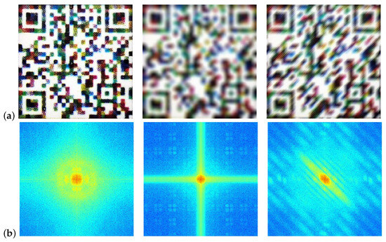
Figure 4.
Spectral representations of security patterns under varying degradation conditions. (a) security patterns; (b) spectral representations. From left to right, each column shows clear, R = 12, and = 45, L = 24, respectively.
Based on these observations, this paper proposes a novel micro-feature degradation and directional energy concentration algorithm (MDDEC) for blur detection in security patterns (see Algorithm 2). Figure 5 presents a visualization of MDDEC for blur detection in security patterns. The algorithm ingeniously combines frequency domain analysis with adaptive spatial processing to achieve high-precision classification of blur types and severity levels. By devising the blur detection mechanism within a systematic spectral analysis framework and using a set of meticulously defined parameters, the algorithm effectively discriminates between different blur types and quantifies their severity. Each parameter plays a specific role in this process: the defocus blur threshold range () quantifies severity levels according to the degree of spectral feature degradation, while the motion blur threshold range () serves a similar purpose for motion-induced blur. The angle offset threshold () differentiates between directional motion blur and isotropic defocus blur by defining an angular tolerance for orientation detection. Meanwhile, the energy distribution ratio error () evaluates the symmetry in the spectral domain, to identify the characteristic patterns of defocus blur. The overall workflow of the algorithm consists of four main stages:
| Algorithm 2 MDDEC: Micro-Feature Degradation and Directional Energy Concentration Algorithm for Blur Detecting | |
| Require: Image Ensure: Blur analysis: pair (type, degree)
| |
| ▹ Defocus blur condition |
| |
| ▹ Motion blur condition |
| |
| ▹ Clear condition |
| |
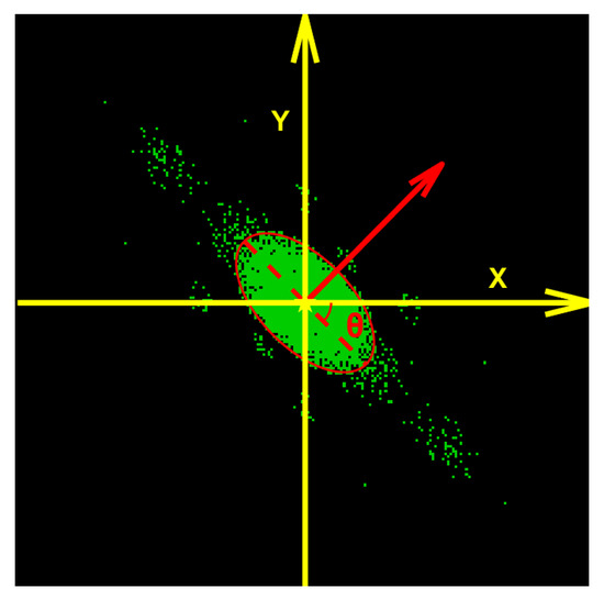
Figure 5.
Visualization of micro-feature degradation and directional energy concentration algorithm for blur detection in security patterns.
Stage 1: Frequency domain analysis
This stage converts the image into a normalized frequency representation, to enhance blur-sensitive features. Converting the image to grayscale () not only reduces the computational complexity, but also preserves the essential structural information. Applying a Hanning window () mitigates spectral leakage by attenuating edge discontinuities. The centered Discrete Fourier Transform (DFT) generates a frequency spectrum , in which blur patterns are more distinguishable. The log-magnitude spectrum compresses the dynamic range to improve the visibility of high-frequency components. Spectral whitening, achieved by normalizing with a Gaussian-smoothed version of the magnitude spectrum, suppresses variations in overall intensity and highlights spatial–frequency structures indicating blur.
Stage 2: Adaptive spectral processing
This stage isolates the salient frequency components related to blur. The analysis is confined to a central region R of the spectrum. This is done to avoid edge artifacts and take advantage of the fact that blur mainly impacts mid-to-high frequencies. Adaptive binarization, which employs Otsu’s method, effectively separates prominent spectral patterns from noise. Subsequently, morphological opening with an elliptical structuring element K refines the binary map . It achieves this by eliminating isolated noise pixels, smoothing region boundaries, and enhancing the connectivity of meaningful spectral structures.
Stage 3: Micro-feature degradation and directional energy concentration
Here, two discriminative features are extracted: Micro-feature degradation metric (A): This metric is calculated as the ratio of non-zero pixels in the binary spectral mask to the total number of pixels in region R. It serves to measure the sparsity of the remaining high-frequency components. A higher degree of blur severity leads to a more significant degradation of fine details, corresponding to lower values of A. Directional energy concentration: The binary map undergoes further processing to retain only the significant regions. The orientation of the largest connected component is obtained through ellipse fitting. This orientation indicates the dominant direction of spectral energy spread, which is a characteristic feature of motion blur. Additionally, the axis ratio is computed by projecting the binary map onto the x- and y-axes. This ratio provides a measure of spectral symmetry. Defocus blur demonstrates high symmetry (), while motion blur exhibits anisotropy.
Stage 4: Hierarchical classification
Utilizing the extracted features, a rule-based classifier differentiates blur conditions as follows: If the dominant orientation is close to horizontal or vertical (within ) and the energy distribution is symmetric (), the blur is categorized as defocus. The severity is determined by comparing A with the thresholds . If a significantly dominant orientation exists (), the blur is classified as motion blur, and the severity is similarly evaluated using . If neither of these conditions is satisfied, the image is classified as clear.
It is important to note that the effectiveness of deblurring algorithms varies depending on the level of blur in the images. While deblurring may improve the accuracy of identification for images with slight or severe blur, it may not result in a significant improvement and may even lead to identification errors for the worst blur patterns. Therefore, it is not recommended to deblur the worst blur patterns, for the sake of efficiency and accuracy. Instead, such problems should be reported directly to the authentication system.
3. Optimized Blind Deblurring Framework
3.1. The Brightness-Gradient Prior in Functional Patterns
The Minimum Brightness Difference (MBD) operator quantifies local brightness variation by computing the minimal intensity deviation within a neighborhood. For an input image T at pixel position i, the MBD is defined as
where is the local neighborhood centered at i, c denotes the color channel (R, G, or B), is the maximum permissible brightness deviation.
The Edge Gradient (EG) feature extracts the gradient magnitude using Sobel filters to emphasize texture and structural discontinuities. For each pixel in T, horizontal and vertical gradients are computed via convolution with Sobel kernels and . A gradient magnitude map is then obtained as
Finally, the edge sparsity measure for a local window is calculated by counting non-zero gradient transitions in both directions:
where denotes the -norm (nonzero count), and , represent the horizontal and vertical discrete gradients, respectively.
The definitions of functional patterns are shown in Figure 6. Figure 7 shows the finder patterns of the patterns and their corresponding prior graphs. It can be observed that the MBD distribution of the blur pattern is much denser. This visual difference is mainly attributed to the structural characteristics of the functional graph. The functional graph comprises three layers: the outermost and innermost layers mainly consist of dark pixels, while the middle layer is close in gray value to bright pixels. The blurring of the pattern causes the dark pixels in the inner and outer layers to spread to the middle layer and compress the bright pixels, resulting in a decrease in their gray value. The binarization process converts bright pixels to zeros once a certain threshold is reached. This results in a higher concentration of dark pixels in the blur pattern, making the MBD appear denser. In addition, the convolution operation of the Sobel operator further accentuates the visual contrast between clear and blur patterns. This operation effectively enhances the edge information of the clear pattern, making the edges more prominent.
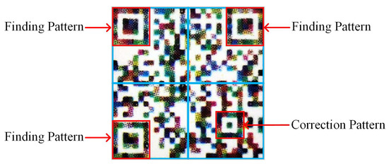
Figure 6.
Functional graphs of the security pattern.
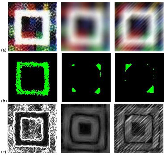
Figure 7.
Visualization of brightness-gradient prior for security patterns in finder patterns. (a) security patterns; (b) MBDs; (c) EGs. From left to right, each column shows clear, R = 12, and = 45, L = 24, respectively.
This paper presents an innovative blind deblurring method to address the problem of blurring of patterns. The steps are as follows: First, partition the input pattern into four sub-regions of the same size. Each sub-region contains a finder pattern or a correction pattern, and these functional graphs have the same size and position in the same version. Then, separately estimate the blur kernel of the functional graphs within each sub-region using fused prior knowledge. Next, the derived blur kernel is used to deblur each sub-region and restore its sharpness. Finally, the four deblurred sub-regions are stitched together to obtain a complete and clear pattern. This method effectively addresses several challenges faced by conventional techniques, such as vulnerability to variable patterned content, non-uniform blur, and high time requirements. Experiments confirmed the superiority of the method in terms of deblurring effect, which enhances the accuracy and reliability of subsequent authentication.
3.2. Defocus Deblurring
This paper presents an innovative brightness-gradient feature fusion to defocus blur patterns. The innovation of this approach is mainly manifested in the following three aspects: First, this method creatively combines the advantages of MBD and EG features. MBD features accurately preserve structural discontinuities through local brightness extremum analysis. Meanwhile, the improved EG features effectively capture texture details with the assistance of the Sobel operator and under the constraint of the norm sparsity. This feature fusion strategy significantly enhances the texture reconstruction accuracy, while maintaining structural integrity. Second, an adaptive pattern optimization mechanism based on MBD is developed. By dynamically screening MBD subsets and generating content-aware masks, it intelligently retains crucial structural information, which is especially evident in the processing of complex texture regions. Finally, a full-frequency domain solution strategy is adopted. The minimization problem is transformed into a closed-form sub-problem based on the Fast Fourier Transform. This enables the potential pattern to be restored in one step, without the need for iterative inverse transformation, thus meeting the requirements of both high-fidelity reconstruction and real-time processing. The specific algorithm process is as follows:
Step 1: The cost function is defined as follows:
where k, C, B, and ⊗ represent the blur kernel, clear pattern, blur pattern, and convolution operator, respectively. The term denotes the regularization constraint of the blur kernel. The weights are denoted by and , and is the regularization constraint of the clear pattern, which is calculated as .
Step 2: Assuming as the intermediate estimate of the blur kernel, the latent pattern can be updated by optimizing the following problem:
Introducing an auxiliary variable W for the gradient , the above problem is approximated by
where is a penalty parameter large enough to satisfy .
Step 3: For the potential pattern and the -th iteration, we define the MBD subset of as . We iteratively apply a threshold to and update C and W.
The MBD is thresholded by setting the threshold parameter as follows:
represents the index set of MBDs in , and the corresponding mask is defined for the subset of MBDs:
Update :
where is the inverse of D. The solution of the gradient subproblem can be expressed as
Step 4: The potential pattern is updated by solving
The Fast Fourier Transform (FFT) can efficiently compute this. The pattern gradients for the horizontal and vertical directions are represented by and , respectively.
Step 5: To update the blur kernel, use the intermediate estimate of the potential pattern:
3.3. Motion Deblurring
This paper puts forward a multi-feature fusion motion deblurring algorithm (see Algorithm 3). The algorithm achieves elimination of the reliance on manual priors through the following technical breakthroughs. First of all, the algorithm innovatively combines three complementary features: (1) Minimum brightness difference (MBD) measures local luminance changes to describe the degree of blur. (2) Edge gradient (EG) features help estimate the blur scale L by detecting patterns in edge degradation. (3) Directional energy concentration (DEC) precisely estimates the blur angle by analyzing the anisotropy of the spectral energy distribution. These three features exhibit strong robustness against noise and non-uniform blur, which is conducive to the accurate blind estimation of motion blur parameters. Then, the algorithm adopts a three-level coarse-to-fine iterative optimization framework within the luminance channel of the YCbCr color space. It commences with initial image restoration via Wiener–Tikhonov regularization during the coarse estimation phase. Subsequently, in the refinement stage, image updating and PSF updating are alternately performed with sparse regularization. After each PSF iteration, non-negativity and energy conservation constraints are automatically imposed. Finally, in the post-processing stage, BM3D denoising is employed, followed by chrominance channel recombination, to generate high-quality RGB output images. Experimental results indicate that this method achieves superior restoration quality, while maintaining excellent adaptability and computational efficiency. The alternating optimization strategy ensures both restoration accuracy and processing speed.
| Algorithm 3 Motion Deblurring via Multi-Feature Fusion |
| Require: Blurred RGB image: Ensure: Deblurred RGB image: Parameters:
|
4. Experiments
4.1. Datasets and Evaluation Metrics
4.1.1. Datasets
Experiments were conducted to verify the performance of our method. The datasets were divided into four categories:
(1) Noised security pattern dataset: Ten digital patterns and 30 smartphone-based patterns (see Table 1) had different types of noise added (brown noise, gaussian noise, salt & pepper noise, and speckle noise), resulting in a dataset of 320 noised patterns and 40 clear patterns. The specific noise parameters employed in the experiment are presented in Table 2.

Table 1.
The smartphones used in the experiments.
Table 2.
The types of noise used in the experiments.
(2) Digital blur security pattern dataset: This contains 100 digital clear patterns of size 464 × 464. To simulate real-world scenarios, we introduced varying degrees of defocus blur (6, 7, 8, 9, 10, 11, and 12) and motion blur (12, 14, 16, 18, 20, 22, and 24) to the aforementioned patterns, resulting in a dataset of 1400 blur patterns and 100 clear patterns.
(3) Smartphone-based artificial blur security pattern dataset: The 100 digital patterns were printed and captured using smartphones. In order to create a more comprehensive dataset, we added defocus blur (6, 7, 8, 9, 10, 11, and 12) and motion blur (12, 14, 16, 18, 20, 22, and 24) to the original set of 100 patterns, resulting in a total of 1500 patterns.
(4) Smartphone-based actual blur security pattern dataset: This contains 40 patterns, obtained from smartphones at different times and circumstances. During the collection process, we invited various users to take photos of blur patterns based on their own habits.
4.1.2. Evaluation Metrics
To assess the efficacy and effectiveness of the deblurring method, objective evaluation metrics including Peak Signal-to-Noise Ratio (PSNR), Structure Similarity Index Measure (SSIM), Pearson Linear Correlation Coefficient (PLCC), Recall, and Runtime were employed. These metrics reflected the performance of the deblurring method in enhancing pattern quality, preserving structural information, maintaining linear correlation, providing security authentication, and enhancing computational efficiency. The pattern to be tested and the corresponding sample pattern are represented by and , respectively. The dimensions of the pattern are denoted by M and N. The metrics are calculated as follows:
(1) PSNR
PSNR is a measure of the ratio between the maximum signal value and the noise point of two patterns. It is measured in decibels (dB), with larger values indicating less distortion.
where represents the logarithmic operation, with a base of 10, and r represents the number of bits per pixel.
(2) SSIM
The quality of a pattern is evaluated by comparing the brightness, contrast, and structure. The SSIM value indicates the degree of similarity between two patterns, with a value of 1 indicating identical patterns.
where and are the means of T and S, respectively. The variances in T and S are and , respectively. The covariance of T and S is . Two constants, and , are also included.
(3) PLCC
PLCC is employed to ascertain the linear correlation between two patterns. The larger the value, the more pronounced the correlation.
where and represent the average value of T and S, respectively.
(4) Recall
The primary objective of the deblurring process is to enhance the accuracy of subsequent authentication and reduce the likelihood of misjudgments. This differs from general image quality evaluation criteria, which prioritize authentication accuracy.
(5) Runtime
In order to guarantee a positive user experience, it is of the utmost importance that smartphone applications are capable of processing images in a timely and efficient manner.
4.2. Experimental Results and Analysis
4.2.1. Robustness Analysis
As shown in Figure 8, a quantitative analysis conducted on the smartphone-based artificial blur dataset revealed that the misclassification rate (MC) of the MDDEC algorithm was predominantly higher in regions characterized by extremely low defocus blur. In these scenarios, blurred images, clear images, and motion blurred images showed a high degree of similarity in their frequency domain features. This similarity posed a significant challenge for the classifier to accurately distinguish among them. It is crucial to note that, given the relatively low intensity of the deblurring processing required for these weakly blurred scenes, even when a suboptimal kernel model is used for restoration, the likelihood of generating significant artifacts, such as severe ringing or over-sharpening, is minimal. Instead, this merely leads to a limited improvement in the restoration effect and a controllable deterioration in visual quality. The misclassification under these specific conditions has an impact on the overall system performance that remains within an acceptable threshold.
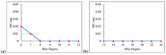
Figure 8.
Misclassification rate (MC) of MDDEC module. (a) defocus blur; (b) motion blur.
In the deblurring algorithm employed in this study, the optimal values of several crucial parameters are affected by multiple factors and must be set in conjunction with the actual scenario and practical experience. To identify the optimal configuration, a series of experiments were conducted. We randomly selected 100 patterns from the smartphone-based artificial blur dataset as validation samples. Figure 9 shows the deblurring effects under different values (0.4, 0.6, 0.8, 1, 1.2, 1.4, 1.6). The experimental results indicate that when equaled 1, both the PSNR and SSIM reached their optimal values. Additionally, is a dynamic threshold, initialized as = 2*. we evaluated the defuzzification effects of parameters and under different combinations (specifically, 25 combinations are presented in Table 3). As shown in Figure 10, the algorithm exhibited the best performance under the configuration of combination No. 14.
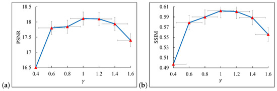
Figure 9.
Performance comparison of different values for smartphone-based artificial blur dataset. (a) PSNR; (b) SSIM.
Table 3.
The multivariate combination schemes of and parameters.
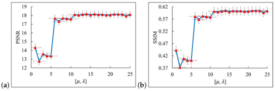
Figure 10.
Performance comparison of different and values for smartphone-based artificial blur dataset. (a) PSNR; (b) SSIM.
4.2.2. Evaluation on Noised Dataset
The CACO technique was demonstrated to be an effective denoising method on a noised dataset (see Figure 11). The CACO method showed significant denoising effects for various types and intensities of noise, with particular efficacy observed for brown noise and salt and pepper noise. As is evident from the error images, in the pattern with superimposed brown noise and salt and pepper noise, there were numerous densely distributed color pixels. After denoising, most of these dense points were removed, leaving only a few scattered small color squares. For patterns containing Gaussian noise and speckle noise, although the macroscopic structure did not change significantly from before to after denoising, at the microscopic detail level, especially in the area of the original fine dots, effective optimization was achieved. For digital patterns (see Table 4), clear patterns had the highest PSNR values in all tests. Following the denoising process, the PSNR values of the patterns were generally higher than those of the noised patterns. The CACO method was particularly effective with the addition of brown noise 0.2 and salt and pepper noise 0.1, indicating effectiveness for all types of noise. The SSIM values of the clear patterns were nearly 1, while the SSIM values of the noised patterns were lower, indicating that the noise had damaged the structure. After denoising, the SSIM values generally improved, especially for brown noise 0.1 and salt and pepper noise 0.1, where the improvement was significant. For example, in the case of salt and pepper noise 0.1, the SSIM value of the pattern was 0.3923. However, after denoising, the SSIM value improved to 0.8851, effectively recovering the structural information of the pattern. Additionally, the PLCC values were also generally improved, close to 1. This indicates that CACO enhanced the linear correlation, especially when dealing with speckle noise 0.2. In all test cases, the Recall values were 100%, and the security system correctly recognized all genuine patterns. For smartphone-based patterns (see Table 5), the PSNR values were generally higher after denoising compared to the noised patterns. Specifically, for brown noise 0.2 and salt and pepper noise 0.1, the PSNR values improved by 3.5315 dB and 5.2452 dB, respectively. The SSIM values also improved after denoising, particularly for brown noise 0.2 and salt and pepper noise 0.1. The PLCC value also exhibited an improvement after denoising, particularly from 0.7959 to 0.9449 in the case of salt and pepper noise 0.1, which better maintained the linear correlation. The Recall values after denoising were higher than those of the noised patterns, with an improvement of 50% and 76.6666% for the cases of brown noise 0.2 and salt and pepper noise 0.1, respectively, effectively recovering the pattern information. In summary, CACO demonstrated the potential for recovering pattern quality, structural similarity, linear correlation, and pattern information. This provides substantial evidence in support of denoising techniques for image processing.
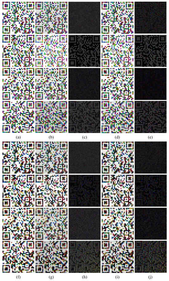
Figure 11.
Visual comparison of CACO on noised dataset. (a) digital clear patterns; (b) digital noised patterns; (c) error images between (a) and (b); (d) digital denoised patterns; (e) error images between (a) and (d). Rows from top to bottom correspond to brown, Gaussian, salt and pepper, and speckle noise, respectively. (f) smartphone-based clear patterns; (g) smartphone-based noised patterns; (h) error images between (f) and (g); (i) smartphone-based denoised patterns; (j) error images between (f) and (i). Rows from top to bottom correspond to brown, Gaussian, salt and pepper, and speckle noise, respectively.
Table 4.
Performance of CACO on digital noised dataset.
Table 5.
Performance of CACO on smartphone-based noised dataset.
4.2.3. Evaluation on Digital Blur Dataset
Figure 12 demonstrates that our method was effective in restoring the pattern under blur conditions. The recovered patterns of other comparative methods displayed artifacts and distorted square color blocks. In some instances, the patterns were distorted to such an extent that the original lines and textures were unrecognizable. As shown in Figure 13, when compared with the blur pattern and the results of other algorithms, the deblurring error images generated by this approach exhibit less structural deviation. This indicates that the restoration result is highly consistent with the overall structure of the clear pattern. Moreover, the error image shows a sparse distribution and weak intensity. Particularly in key areas such as edges and textures, the error was significantly reduced, highlighting the precise restoration ability for details and the excellent artifact suppression effect. As shown in Figure 14, our method demonstrated satisfactory performance when confronted with slight blur patterns, as evidenced by its high PSNR, SSIM, and PLCC values. In contrast, Wen et al.’s [10] and Pan et al.’s [6] methods also achieved some effect, although they were slightly inferior to the former two. Bai et al.’s [8], Alexander et al.’s [12], and Zheng et al.’s [33] methods performed in a more average manner. In the case of severe blur patterns, our method outperformed the others in terms of PSNR, SSIM, and PLCC values, while the Recall remained stable and high. For example, at a blur level of 12, our method achieved a PSNR value of 20.9331. Similarly, the SSIM, PLCC, and Recall values exhibited a similar trend. Figure 15 demonstrates the successful management of motion blur by our method. Our method achieved the highest PSNR values across almost all blur levels. Notably, at a blur level 24, our method achieved a PSNR value of 18.2477, which was significantly higher than the best value of 14.9142 achieved by Zheng et al. [33]. Additionally, our method performed well in SSIM. For PLCC, our method reached 0.97 at blur levels 12 to 16, indicating that the deblurred pattern closely resembled the original pattern and recovered a substantial portion of the original image information. Even at the highest blur level of 24, our method still achieved a high PLCC value of 0.9381, which was significantly higher than the best value among other methods, the 0.8581 of Bai et al. [8]. Additionally, our method achieved a Recall value of 100% for blur levels 12 to 20. Although the Recall value decreased slightly at higher blur levels, our method maintained a high percentage. For example, at blur level 22, the Recall value of our method was 70%, while the Recall values of all other methods were 0%. In conclusion, our method demonstrated efficacy in a number of evaluation metrics when processing digital defocus blur or motion blur. Its advantages were particularly evident when dealing with patterns exhibiting higher blur levels.
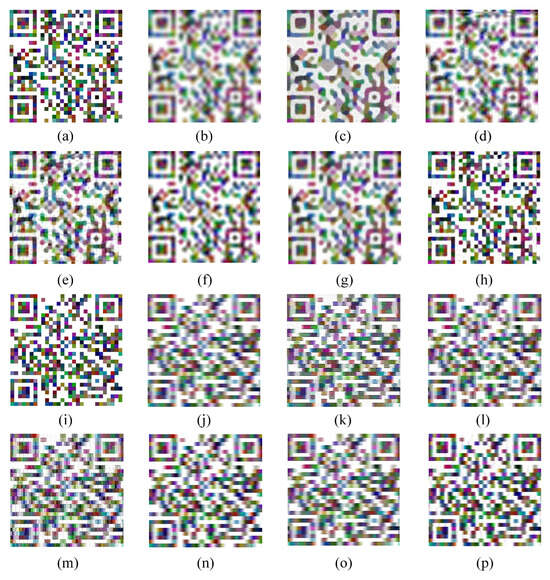
Figure 12.
Visual comparison on digital blur dataset. (a) clear; (b) defocus blur; (c) Pan et al. [6]; (d) Bai et al. [8]; (e) Wen et al. [10]; (f) Alexander et al. [12]; (g) Zheng et al. [33]; (h) ours; (i) clear; (j) motion blur; (k) Pan et al. [6]; (l) Bai et al. [8]; (m) Wen et al. [10]; (n) Alexander et al. [12]; (o) Zheng et al. [33]; (p) ours.
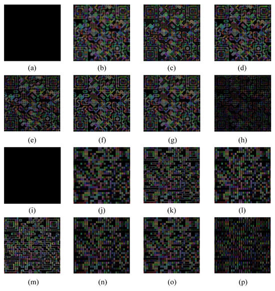
Figure 13.
Error images on digital blur dataset. (a) clear; (b) defocus blur; (c) Pan et al. [6]; (d) Bai et al. [8]; (e) Wen et al. [10]; (f) Alexander et al. [12]; (g) Zheng et al. [33]; (h) ours; (i) clear; (j) motion blur; (k) Pan et al. [6]; (l) Bai et al. [8]; (m) Wen et al. [10]; (n) Alexander et al. [12]; (o) Zheng et al. [33]; (p) ours.
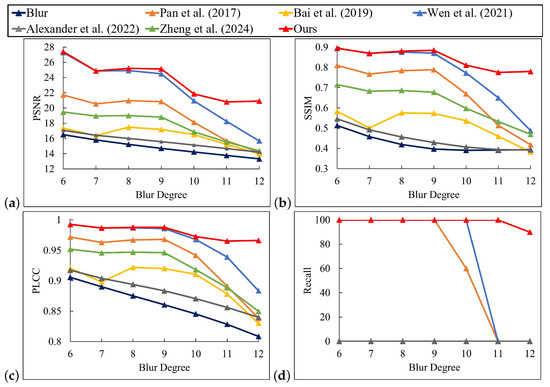
Figure 14.
Performance comparison of different methods on digital defocus blur dataset [6,8,10,12,33]. (a) PSNR; (b) SSIM; (c) PLCC; (d) Recall.
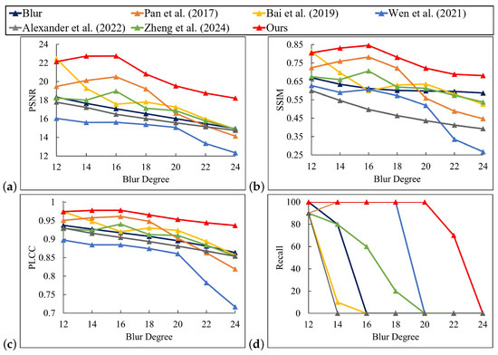
Figure 15.
Performance comparison of different methods on digital motion blur dataset [6,8,10,12,33]. (a) PSNR; (b) SSIM; (c) PLCC; (d) Recall.
4.2.4. Evaluation on Smartphone-Based Artificial Blur Dataset
Six deblurring methods were used to process the smartphone-based artificial blur dataset, and the experimental results are shown in Figure 16 and Figure 17. All types of deblurring algorithms tend to generate artifacts. However, the artifacts produced by the method proposed in this paper were less prominent. They were more visually inconspicuous, fragmented in form, and sparsely dispersed. Meanwhile, the overall pixel intensity of its error image was lower, the fidelity was higher, and the comprehensive performance was superior. The methods of Pan et al. [6], Bai et al. [8], Alexander et al. [12], and Zheng et al. [33] resulted in significant distortion when processing severe blur patterns. The processed patterns differed significantly from the original clear patterns in terms of the texture and lines of the pattern. While the method of Wen et al. [10] performed better in processing the details of motion blur patterns, it introduced significant noise and artifacts. Moreover, it was not effective in processing high-intensity defocus blur. In contrast, our method demonstrated superior restoration results in the deblurring process. Figure 18 and Figure 19 present the quantitative comparison results between our method and five other compared methods. Our method slightly outperformed the others in four objective evaluation metrics, namely PSNR, SSIM, PLCC, and Recall. It performed particularly well in handling highly blurred patterns and is applicable to various types of blur patterns. All methods generally exhibited a decrease in PSNR values as the degree of blur increased. However, our method achieved the highest PSNR values for both datasets, showing its advantage in improving pattern clarity. For the SSIM metric, our method maintained the highest value at almost all blur levels, indicating its superior ability to preserve the similarity of the pattern structure. Our method also achieved the highest value for the PLCC metric, demonstrating excellent performance in reconstructing pattern details and maintaining overall consistency. Additionally, our method achieved 100% Recall under almost all levels of blur, indicating its effectiveness in restoring patterns with different levels of blur.
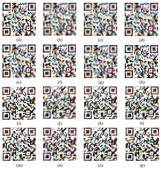
Figure 16.
Visual comparison on smartphone-based artificial blur dataset. (a) clear; (b) defocus blur; (c) Pan et al. [6]; (d) Bai et al. [8]; (e) Wen et al. [10]; (f) Alexander et al. [12]; (g) Zheng et al. [33]; (h) ours; (i) clear; (j) motion blur; (k) Pan et al. [6]; (l) Bai et al. [8]; (m) Wen et al. [10]; (n) Alexander et al. [12]; (o) Zheng et al. [33]; (p) ours.
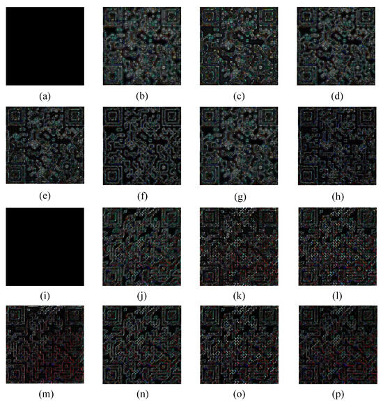
Figure 17.
Error images on smartphone-based artificial blur dataset. (a) clear; (b) defocus blur; (c) Pan et al. [6]; (d) Bai et al. [8]; (e) Wen et al. [10]; (f) Alexander et al. [12]; (g) Zheng et al. [33]; (h) ours; (i) clear; (j) motion blur; (k) Pan et al. [6]; (l) Bai et al. [8]; (m) Wen et al. [10]; (n) Alexander et al. [12]; (o) Zheng et al. [33]; (p) ours.
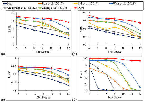
Figure 18.
Performance comparison of different methods on smartphone-based artificial defocus blur dataset [6,8,10,12,33]. (a) PSNR; (b) SSIM; (c) PLCC; (d) Recall.
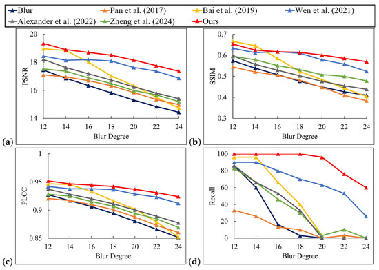
Figure 19.
Performance comparison of different methods on smartphone-based artificial motion blur dataset [6,8,10,12,33]. (a) PSNR; (b) SSIM; (c) PLCC; (d) Recall.
4.2.5. Evaluation on Smartphone-Based Actual Blur Dataset
Actual blur patterns may have multiple complex blur types, which increases the difficulty of deblurring (see Figure 20 and Figure 21). In the highly demanding task of processing severely blurred images, the deblurring algorithm presented in this paper exhibited remarkable reconstruction performance. The restoration outcomes of this method were markedly superior to those of other algorithms, effectively preventing severe artifacts and structural distortions. It also performed remarkably well in suppressing distortion, maintaining structural stability, and preserving color fidelity. Further analysis of the error images provided quantitative evidence for the above visual advantages. The residual images generated by the algorithm had the lowest overall pixel intensity, and the error values in the detailed regions were significantly smaller than those of the comparison methods, fully demonstrating its exceptional capabilities in reconstruction accuracy and detail preservation. As seen in Figure 22, our method achieved a remarkable result of 18.4349 in terms of PSNR, which significantly exceeded the other five compared methods. Meanwhile, on SSIM, our method and Zheng et al.’s [33] method obtained high scores of 0.6212 and 0.6368, respectively, which were both ahead of the other compared methods. In addition, our method also achieved 0.9432 in terms of PLCC, surpassing the other methods. It is particularly noteworthy that in the key metric of recall, our method achieved a perfect score of 100%, significantly exceeding the methods of Pan et al. [6], Bai et al. [8], and Alexander et al. [12]. The latter two had a recall of only 92.5%. This outstanding performance not only proves the efficient ability of our method in recovering the content of blur patterns but also reflects its strong potential in practical applications. Although the method in this paper achieved excellent results for most of the performance indicators, there is still room for improvement in maintaining the structure and details of the security pattern. This may be due to the fact that the design of the algorithm focuses too much on the clarity enhancement of a single blur type, while the ability to retain detail information and accurately reconstruct in the case of multiple types of blur needs to be further strengthened.
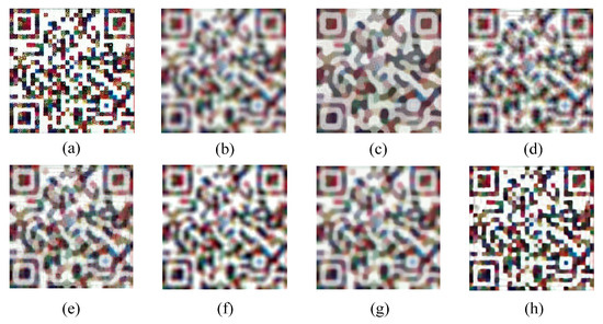
Figure 20.
Visual comparison on smartphone-based actual blur dataset. (a) clear; (b) defocus blur; (c) Pan et al. [6]; (d) Bai et al. [8]; (e) Wen et al. [10]; (f) Alexander et al. [12]; (g) Zheng et al. [33]; (h) ours.
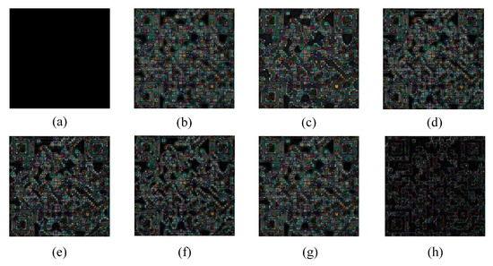
Figure 21.
Error images on smartphone-based actual blur dataset. (a) clear; (b) defocus blur; (c) Pan et al. [6]; (d) Bai et al. [8]; (e) Wen et al. [10]; (f) Alexander et al. [12]; (g) Zheng et al. [33]; (h) ours.
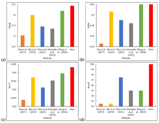
Figure 22.
Performance comparison of different methods on smartphone-based actual blur dataset [6,8,10,12,33]. (a) PSNR; (b) SSIM; (c) PLCC; (d) Recall.
Figure 23 shows the notable discrepancy in the runtimes of various methods. In this study, the subject under investigation was an image processing system based on a smartphone platform. The processing speed of the proposed method is sufficient for near real-time operation. Specifically, the processing time for a single frame is approximately 16 s, which can stably support non-real-time interactive applications, such as photo post-processing. To continuously optimize efficiency, subsequent technical solutions could be implemented, including multi-threaded parallel scheduling, low-level code refactoring (using C++/Metal/Vulkan), and dynamic convergence mechanisms—automatically terminating iterations when the calculation results reach a preset precision threshold to achieve a more efficient processing flow.
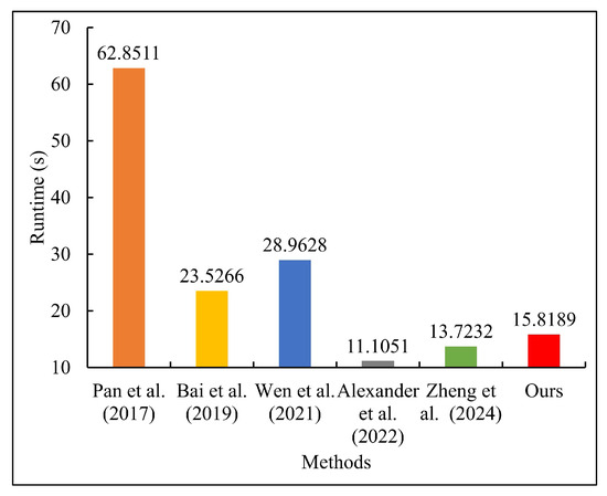
Figure 23.
Comparison of runtimes [6,8,10,12,33].
5. Conclusions
In authentication and traceability systems, the operational effectiveness and precision of security patterns are crucial determinants of their practical utility. To address this need, we undertook a comprehensive investigation and developed an enhanced methodology that systematically incorporates domain-specific prior knowledge. This method effectively addresses the deblurring problem and significantly improves processing speed, providing strong technical support for the clear authentication and wide application of patterns. Despite these advances, we recognize that there are still some unresolved challenges in this research area. Future work will focus on the following key areas: (1) Validate the robustness of the deblurring method by expanding the dataset to include more pattern variations in real-world scenarios. (2) Expand the applicability to other types of patterns. It is important to note that although existing methods have both efficiency and reliability advantages, they encounter performance bottlenecks when dealing with extreme mutations or complex non-uniform blurring. Additionally, it is particularly challenging to directly process security patterns lacking structural features. Consequently, subsequent research will focus on exploring adaptive prior learning mechanisms and weak structural feature extraction techniques. The aim is to improve the algorithm’s generalization ability in complex anti-counterfeiting scenarios, thus providing a better solution for optimizing anti-counterfeiting pattern technology.
Author Contributions
Conceptualization, T.W., H.Z., Z.X. and T.T.; methodology, T.W. and H.Z.; software, T.W., H.Z. and Z.X.; validation, T.W.; formal analysis, T.W., H.Z. and T.T.; investigation, T.W. and H.Z.; resources, T.W., H.Z. and T.T.; data curation, T.W., Z.X. and T.T.; writing—original draft preparation, T.W. and H.Z.; writing—review and editing, T.W., Z.X. and H.Z.; visualization, T.W., H.Z., Z.X. and T.T.; supervision, H.Z.; project administration, H.Z.; funding acquisition, and H.Z. All authors have read and agreed to the published version of the manuscript.
Funding
This work was supported by the Natural Science Foundation of Hubei Province of China (Grant No. 2022CFB536) and the National Natural Science Foundation of China (Grant No. 62367006).
Data Availability Statement
The original contributions presented in the study are included in the article; further inquiries can be directed to the corresponding author.
Conflicts of Interest
The authors declare no conflicts of interest.
References
- Guo, Z.; Wang, S.; Zheng, Z.; Sun, K. Printer source identification of quick response codes using residual attention network and smartphones. Eng. Appl. Artif. Intell. 2024, 131, 107822. [Google Scholar] [CrossRef]
- Yan, Y.; Zou, Z.; Xie, H.; Gao, Y.; Zheng, L. An IoT-based security system using visual features on QR code. IEEE Internet Things J. 2021, 8, 6789–6799. [Google Scholar] [CrossRef]
- Zheng, H.; Zhou, C.; Li, X.; Wang, T.; You, C. Forgery detection for anti-counterfeiting patterns using deep single classifier. Appl. Sci. 2023, 13, 8101. [Google Scholar] [CrossRef]
- Chen, J.; Dong, L.; Wang, R.; Yan, D.; Sun, W.; Fan, H. Physical anti-copying semi-robust random watermarking for QR code. In Digital Forensics and Watermarking; Zhao, X., Tang, Z., Comesaña-Alfaro, P., Piva, A., Eds.; Springer: Cham, Switzerland, 2023; pp. 131–146. [Google Scholar]
- Xie, N.; Chen, J.; Chen, Y.; Hu, J.; Zhang, Q.; Chen, C.; Huang, L. Detection of information hiding at anti-copying 2d barcodes. IEEE Trans. Circuits Syst. Video Technol. 2022, 32, 437–450. [Google Scholar] [CrossRef]
- Pan, J.; Hu, Z.; Su, Z.; Yang, M. L0-regularized intensity and gradient prior for deblurring text images and beyond. IEEE Trans. Pattern Anal. Mach. Intell. 2017, 39, 342–355. [Google Scholar] [CrossRef]
- Anwar, S.; Huynh, C.; Porikli, F. Image deblurring with a class-specific prior. IEEE Trans. Pattern Anal. Mach. Intell. 2019, 41, 2112–2130. [Google Scholar]
- Bai, Y.; Cheung, G.; Liu, X.; Gao, W. Graph-based blind image deblurring from a single photograph. IEEE Trans. Image Process. 2019, 28, 1404–1418. [Google Scholar] [CrossRef]
- Bai, Y.; Jia, H.; Jiang, M.; Liu, X.; Xie, X.; Gao, W. Single-image blind deblurring using multi-scale latent structure prior. IEEE Trans. Circuits Syst. Video Technol. 2020, 30, 2033–2045. [Google Scholar] [CrossRef]
- Wen, F.; Ying, R.; Liu, Y.; Liu, P.; Truong, T. A simple local minimal intensity prior and an improved algorithm for blind image deblurring. IEEE Trans. Circuits Syst. Video Technol. 2021, 31, 2923–2937. [Google Scholar] [CrossRef]
- Zhang, M.; Fang, Y.; Ni, G.; Zeng, T. Pixel screening based intermediate correction for blind deblurring. In Proceedings of the 2022 IEEE/CVF Conference on Computer Vision and Pattern Recognition, New Orleans, LA, USA, 18–24 June 2022; pp. 1–9. [Google Scholar]
- Alexander, G.B.; Fayolle, P.A. Black-box image deblurring and defiltering. Signal Process. Image Commun. 2022, 108, 0923–5965. [Google Scholar] [CrossRef]
- Shao, W. Revisiting the regularizers in blind image deblurring with a new one. IEEE Trans. Image Process. 2023, 32, 3994–4009. [Google Scholar] [CrossRef]
- Cai, Z.; Fang, M.; Li, Z.; Ming, J.; Wang, H. Blind remote sensing image deblurring based on local maximum high-frequency coefficient prior and graph regularization. IEEE J. Sel. Top. Appl. Earth Obs. Remote Sens. 2024, 17, 18577–18592. [Google Scholar] [CrossRef]
- Huang, G.; Zhang, H.; Guo, J.; Wang, J.; Zhang, Y.; Wang, Y. Remote sensing image deblurring based on differential lorentzian PSF model. IEEE Geosci. Remote Sens. Lett. 2025, 22, 1–5. [Google Scholar] [CrossRef]
- Ren, W.; Zhang, J.; Pan, J.; Liu, S.; Ren, J.S.; Du, J.; Cao, X.; Yang, M.-H. Deblurring dynamic scenes via spatially varying recurrent neural networks. IEEE Trans. Pattern Anal. Mach. Intell. 2021, 44, 3974–3987. [Google Scholar] [CrossRef] [PubMed]
- Bono, F.M.; Radicioni, L.; Cinquemani, S.; Conese, C.; Tarabini, M. Development of soft sensors based on neural networks for detection of anomaly working condition in automated machinery. In Proceedings of the NDE 4.0, Predictive Maintenance, and Communication and Energy Systems in a Globally Networked World, Long Beach, CA, USA, 6 March–11 April 2022; Volume 1204907. [Google Scholar]
- Ma, H.; Liu, S.; Liao, Q.; Zhang, J.; Xue, J. Defocus image deblurring network with defocus map estimation as auxiliary task. IEEE Trans. Image Process. 2022, 31, 216–226. [Google Scholar] [CrossRef] [PubMed]
- Que, J.; Lu, C. Lightweight and dynamic deblurring for IoT-enabled smart cameras. IEEE Internet Things J. 2022, 9, 20693–20705. [Google Scholar] [CrossRef]
- Wang, M.; Chen, K.; Lin, F. Multi-residual generative adversarial networks for QR code deblurring. In Proceedings of the 2022 International Conference on Electronic Information Technology, Chengdu, China, 18–20 March 2022; pp. 589–594. [Google Scholar]
- Li, Z.; Gao, Z.; Yi, H.; Fu, Y.; Chen, B. Image deblurring with image blurring. IEEE Trans. Image Process. 2023, 32, 5595–5609. [Google Scholar] [CrossRef] [PubMed]
- Sharif, S.; Naqvi, R.; Ali, F.; Biswas, M. Darkdeblur: Learning single-shot image deblurring in low-light condition. Expert Syst. Appl. 2023, 222, 119739. [Google Scholar] [CrossRef]
- Mao, Y.; Wan, Z.; Dai, Y.; Yu, X. Deep idempotent network for efficient single image blind deblurring. IEEE Trans. Circuits Syst. Video Technol. 2023, 33, 172–185. [Google Scholar] [CrossRef]
- Liang, P.; Jiang, J.; Liu, X.; Ma, J. Decoupling image deblurring into twofold: A hierarchical model for defocus deblurring. IEEE Trans. Comput. Imaging 2024, 10, 1207–1220. [Google Scholar] [CrossRef]
- Quan, Y.; Wu, Z.; Xu, R.; Ji, H. Deep single image defocus deblurring via Gaussian kernel mixture learning. IEEE Trans. Pattern Anal. Mach. Intell. 2024, 46, 11361–11377. [Google Scholar] [CrossRef]
- Feng, Y.; Yang, Y.; Fan, X.; Zhang, Z.; Zhang, J. A multiscale generalized shrinkage threshold network for image blind deblurring in remote sensing. IEEE Trans. Geosci. Remote Sens. 2024, 62, 5611316. [Google Scholar] [CrossRef]
- Zhuang, K.; Li, Q.; Yuan, Y.; Wang, Q. Multi-domain adaptation for motion deblurring. IEEE Trans. Multimed. 2024, 26, 3676–3688. [Google Scholar] [CrossRef]
- Shi, Y.; He, B.; Zhu, M.; Zhang, L. Fast linear motion deblurring for 2d barcode. Optik 2020, 219, 164902. [Google Scholar] [CrossRef]
- Rioux, G.; Scarvelis, C.; Choksi, R.; Hoheisel, T.; Maréchal, P. Blind deblurring of barcodes via Kullback-Leibler divergence. IEEE Trans. Pattern Anal. Mach. Intell. 2021, 43, 77–88. [Google Scholar] [CrossRef] [PubMed]
- Chen, R.; Zheng, Z.; Yu, Y.; Zhao, H.; Ren, J.; Tan, H. Fast restoration for out-of-focus blurred images of QR code with edge prior information via image sensing. IEEE Sens. J. 2021, 21, 18222–18236. [Google Scholar] [CrossRef]
- Chen, R.; Zheng, Z.; Pan, J.; Yu, Y.; Zhao, H.; Ren, J. Fast blind deblurring of qr code images based on adaptive scale control. Mobile Netw. Appl. 2021, 26, 2472–2487. [Google Scholar] [CrossRef]
- Li, J.; Zhang, D.; Zhou, M.; Cao, Z. A motion blur QR code identification algorithm based on feature extracting and improved adaptive thresholding. Neurocomputing 2022, 493, 351–361. [Google Scholar] [CrossRef]
- Zheng, H.; Guo, Z.; Liu, C.; Li, X.; Wang, T.; You, C. Blind deblurring of anti-counterfeiting QR codes using intensity and gradient prior of positioning patterns. Vis. Comput. 2024, 40, 441–455. [Google Scholar] [CrossRef]
- Xu, B.; Jin, R.; Li, J. Robust and fast QR code images deblurring via local maximum and minimum intensity prior. Vis. Comput. 2024, 40, 8809–8823. [Google Scholar] [CrossRef]
Disclaimer/Publisher’s Note: The statements, opinions and data contained in all publications are solely those of the individual author(s) and contributor(s) and not of MDPI and/or the editor(s). MDPI and/or the editor(s) disclaim responsibility for any injury to people or property resulting from any ideas, methods, instructions or products referred to in the content. |
© 2025 by the authors. Licensee MDPI, Basel, Switzerland. This article is an open access article distributed under the terms and conditions of the Creative Commons Attribution (CC BY) license (https://creativecommons.org/licenses/by/4.0/).