Article

Quantitative Hazard Assessment of Mining-Induced Seismicity Using Spatiotemporal b-Value Dynamics from Microseismic Monitoring

1
Lanzhou Institute of Seismology, China Earthquake Administration, Lanzhou 730000, China
2
Gansu Earthquake Agency, Lanzhou 730000, China
3
Shaanxi Earthquake Agency, Xi’an 710068, China
*
Author to whom correspondence should be addressed.
Appl. Sci. 2025, 15(18), 10073; https://doi.org/10.3390/app151810073
Submission received: 5 August 2025 / Revised: 12 September 2025 / Accepted: 12 September 2025 / Published: 15 September 2025
(This article belongs to the Special Issue Earthquake Detection, Forecasting and Data Analysis)

Abstract

Mining-induced seismicity poses significant safety risks in deep coal mining operations, necessitating advanced monitoring and accurate hazard assessment. Based on 15,584 microseismic events from a coal mine in Gansu, China, in 2024, this study investigates the spatiotemporal characteristics of mining-induced seismicity and its quantitative relationship with excavation disturbances. The methodology integrates Gaussian Mixture Model (GMM) clustering analysis with maximum likelihood estimation of b-value. Key findings include: (1) GMM clustering effectively identifies distinct seismic zones under different stress states, with significant variations in b-values (0.64–0.70). Low b-value zones correspond to high stress concentration and potential for strong events, enabling refined hazard assessment; (2) The time-sliding window analysis reveals the dynamic evolution of the b-value, which exhibits a clear negative correlation with high-energy seismic activity. When the b-value drops sharply to 0.6 or below, the likelihood of high-energy events increases markedly. Notably, 7 out of 8 high-energy seismic events occurred below this threshold. (3) Seismicity migrates with working face advancement, with monthly excavation length positively correlating with seismic energy release, confirming excavation as the primary trigger. This b-value spatiotemporal analysis framework provides scientific basis for early warning and mining optimization in deep coal mines.

1. Introduction

With the large-scale exploitation of coal resources and the increasing depth of underground mining, mining-induced seismicity has emerged as a major dynamic hazard. Its increasing frequency and destructive potential now pose severe threats to coal mine safety [1]. Mining-induced seismicity refers to seismic vibrations that occur within coalfield development areas, caused by the combined effects of regional stress fields and mining disturbances, which lead to the sudden release of locally accumulated energy in the rock mass [2,3,4]. Such mining disturbances encompass both operational factors (e.g., longwall face advancement, blasting) and adverse geological anomalies (e.g., faults, massive sandstone roofs), which often complicate the mining process and increase operational costs [5]. These seismic events frequently cause equipment damage, production interruption, and even casualties, leading to significant economic and social consequences [6]. Therefore, real-time monitoring of seismic activity using a microseismic monitoring system, coupled with the identification of potential hazards based on seismic parameters, is a key strategy for ensuring safe mine operations [3,7,8,9].
The Gutenberg–Richter (G–R) relationship is an empirical formula widely used to describe the magnitude distribution of seismic events in a specific region and time period [10]. It is expressed mathematically as:
l g N   =   a bM ,
where M is the magnitude, N is the number of seismic events with magnitudes greater than or equal to M, and a and b are empirical parameters representing regional seismic activity. The a-value reflects the general level of seismic activity: a higher a-value indicates a greater frequency of events, which may be associated with stress accumulation or increased fault system activity. In mining contexts, temporal variations in a-value may indicate the extent to which mining activities alter the regional stress field. The b-value indicates the relative proportion of small to large events and correlates strongly with regional stress state [11]. Numerous studies have shown that the b-value is negatively correlated with crustal stress levels, with lower b-values typically associated with higher stress concentrations and thus an elevated probability of future strong seismic events [12]. Consequently, temporal monitoring of the b-value is considered an effective tool for forecasting larger seismic events.
The applicability of the G–R relationship to mining-induced seismicity is well-established [13]. Boettcher et al. confirmed G–R relationship compliance for mining-induced events below MW −1.3 using 12-year data from TauTona Gold Mine, South Africa [14]. Based on microseismic data from the Creighton and Kidd hard-rock mines in Canada, Ma et al. proposed that inflection points in b-value trends can serve as early warning indicators for impending high-magnitude events [15]. Huang et al. demonstrated significantly shortened stress accumulation cycles in induced seismicity at Sichuan, China, shale gas field due to anthropogenic activities [16]. These studies validate the application of b-value analysis in assessing mining-induced seismic hazards. Spatiotemporal distribution of mining-induced seismicity directly reflects local stress states and fracture characteristics. Traditional seismic zoning methods often rely on qualitative judgments based on tectonic backgrounds, which are inadequate for high-frequency, strongly heterogeneous mining seismicity [17]. Clustering analysis, as a data-driven and objective approach, provides a promising method for identifying the spatial patterns of mining-induced seismicity [18]. Hudyma utilized spatial clustering techniques to interpret microseismic activity patterns [18]. Wu et al. applied the nearest-distance clustering algorithm to analyze the spatiotemporal distribution of microseismic events [17]. Chen developed the KST-DBSCAN algorithm, demonstrating that spatiotemporal density-based clustering can significantly improve the accuracy of seismic early warning [19]. Despite the progress made, several limitations remain: (1) the traditional G–R relationship relies primarily on magnitude, neglecting other seismological parameters such as energy, which may result in incomplete stress assessments; (2) b-value calculations are often applied to the entire mining area, lacking detailed spatial differentiation; and (3) the quantitative relationship between seismicity and excavation disturbances is still insufficiently explored.
To address these issues, this study utilizes microseismic data collected in 2024 from a coal mine in Gansu Province, China. A methodology integrating the Gaussian Mixture Model (GMM) clustering with spatiotemporal b-value analysis is proposed. GMM clustering is first applied to delineate seismically homogeneous subregions. The b-value characteristics are then calculated for each cluster, and their temporal evolution is analyzed using a time-sliding window approach. By quantitatively linking these spatiotemporal b-value dynamics to mining-induced stress disturbances, this study aims to establish a refined framework for seismic risk assessment and early warning in deep coal mines.

2. Materials and Methods

2.1. Seismic Catalog Data

This study focuses on a coal mine located in Gansu Province, China, with its regional context illustrated in the topographic map in Figure 1a. The mine is situated within the Loess Plateau, characterized by highly dissected terrain and complex geomorphological features. Surface elevations range from 1827 m to 2380 m, sloping from north to south, with a local relative relief of approximately 200–550 m. The key geological units, shown in the simplified stratigraphic column in Figure 1c, consist of two mineable seams: the upper Oil-A Formation, which serves as a protective seam, and the underlying Coal Seam II, the primary production seam. The mine is developed at two production levels and subdivided into three mining districts, with their outlines shown in Figure 1b [20]. During 2024, mining operations were concentrated in District I on two key working faces: 6116 and 6126-1. Both working faces are oriented along an east–west strike and were advanced from east to west. Working face 6116 has a strike length of approximately 958.2 m, and extraction ceased on 31 July 2024. Working face 6126-1, with a strike length of approximately 991.2 m and remained in continuous production throughout the year. The mine is equipped with the Seismological Observation System (SOS) microseismic monitoring network and 14 surface-based ALLSEIS-4C three-component short-period seismic stations. The spatial distribution of these stations across the mining area is shown in Figure 1b.
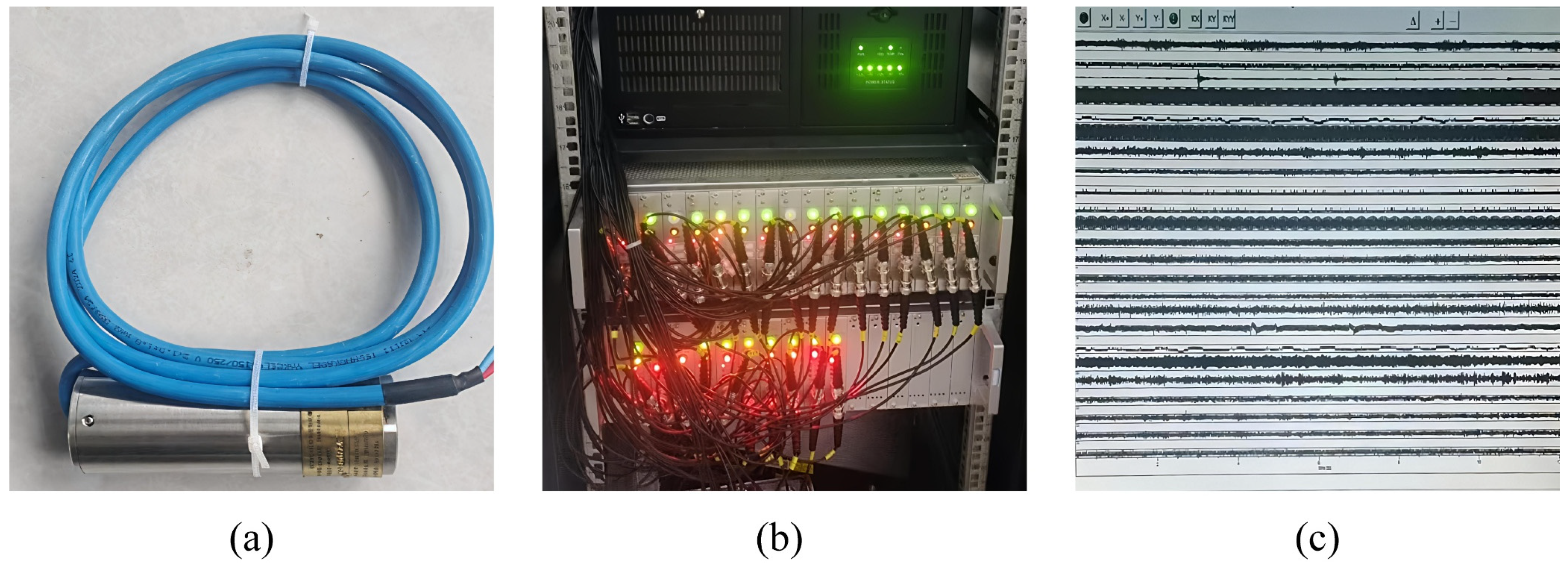
The data used in this study were primarily collected by the SOS microseismic monitoring system, which was manufactured by the Central Mining Institute of Poland and deployed by the China University of Mining and Technology. The main components of this system are shown in Figure 2, including the DLM2001 geophones for signal acquisition, a central server for data transmission and storage, and specialized software for data processing and analysis. Based on its application across multiple mines, the system has been proven capable of accurately locating the three-dimensional coordinates, occurrence time, and energy of microseismic events with energy E > 100 J [21,22,23]. Additionally, the waveform characteristics enable the identification of event types. With optimized geophone placement in both surface and underground configurations, the system achieves localization errors of less than 20 m horizontally and less than 30 m vertically. For purely underground geophone networks, horizontal errors remain less than 20 m, while vertical errors increase to less than 70 m. The SOS system operates within a frequency range of 0.1 to 600 Hz, which ensures comprehensive coverage of microseismic activity throughout the mine and allows for enhanced monitoring of key zones [22].
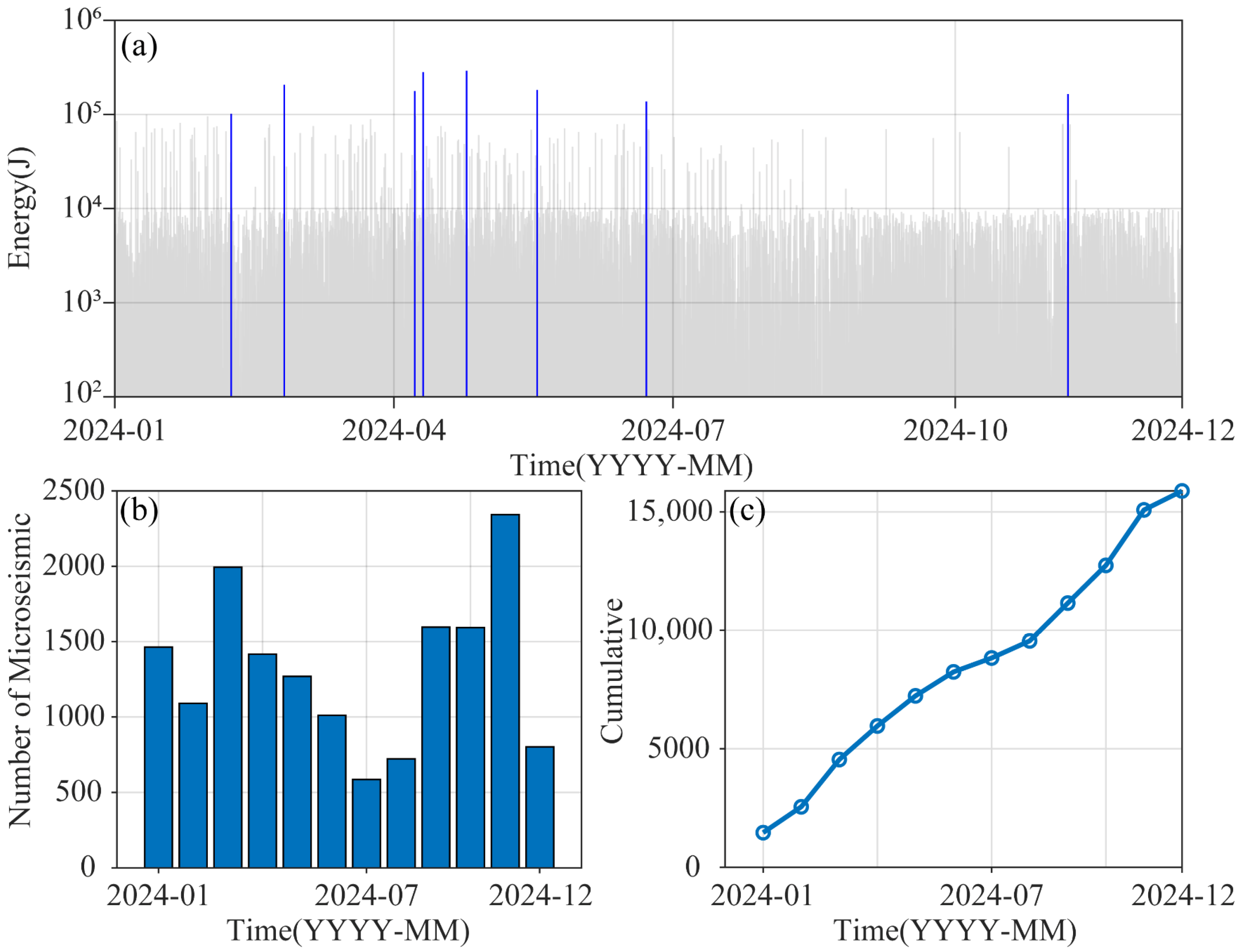
A total of 15,584 mining-induced seismic events were detected within the monitored area of the mine from 1 January to 14 December 2024, based on microseismic monitoring data. The maximum recorded energy was 2.91 × 10⁵ J, the minimum was 1.04 J, and the average energy was 2.03 × 10³ J. As shown in Table 1, the majority of events had energies concentrated in the range of 102–103 J, accounting for 48.60% of all recorded seismic events. Events with energies exceeding 105 J were extremely rare, comprising only 0.05% of the total.
According to the plot of seismic energy versus time, high-energy microseismic events with energy greater than 105 J were relatively scattered and primarily occurred during the first half of 2024 (Figure 3a). As shown in Figure 3b, the number of microseismic events was relatively low from July to August 2024. From September to November 2024, the recorded seismic activity increased; however, high-energy events (>105 J) remained rare, with most events having energy levels below 104 J. The cumulative frequency curve in Figure 3c indicates that the total number of events generally exhibited a steady upward trend.

2.2. Clustering Method

The Gaussian Mixture Model (GMM) is a probabilistic clustering method that assumes a dataset is generated by a mixture of Gaussian distributions, with each Gaussian distribution representing a potential cluster. As a soft clustering method, GMM estimates the probability that each data point belongs to each cluster, which allows for more flexible and accurate clustering performance. Assuming there are K Gaussian components, each characterized by its mean vector μ k , covariance matrix Σ k , and mixing coefficient π k , each data point xi in the dataset is assumed to be generated from one of these K components. The model formula for GMM is as follows:
p x   = k = 1 k π k f ( x | μ k , Σ k ) ,
where f ( x | μ k , Σ k ) denotes the probability density function of the k-th Gaussian component, representing the likelihood of data point x under component k. The mixing coefficients π k satisfy k = 1 k π k = 1.
When applying GMM clustering, the number of clusters K must be specified in advance. Model parameters are typically estimated using the Expectation-Maximization (EM) algorithm, an iterative optimization technique suitable for probabilistic models with latent variables or incomplete data [24]. In the context of GMM, the latent variables correspond to the probabilities of data points belonging to each Gaussian component. The EM algorithm consists of two primary steps: Expectation step (E-step): Given the current model parameters ( μ k , Σ k , π k ), compute the posterior probabilities that each data point belongs to each Gaussian component. Maximization step (M-step): Update the model parameters based on the posterior probabilities computed in the E-step. These two steps are iteratively executed until convergence, typically determined by changes in the log-likelihood function or a preset number of iterations. During this process, the model parameters are progressively refined to better fit the data. Selecting an appropriate number of components K is crucial in GMM applications. Model selection criteria such as the Akaike Information Criterion (AIC) [25] or the Bayesian Information Criterion (BIC) [26] are commonly employed to evaluate the model fit under different values of K. Cross-validation methods can also be used to determine the optimal K. The formulas for AIC and BIC are as follows:
AIC   =   2 ln L θ   +   2 k ,
BIC = 2 ln L θ + k ln N ,
where L(θ) is the maximized likelihood function under the estimated model, k is the number of estimated parameters, and N is the number of data points.

2.3. b-Value Estimation Method

To establish a quantitative relationship between the energy and frequency of mine-induced seismic events, this study adopts an improved version of the classical G–R relationship by replacing the magnitude M with the logarithmic energy lgE as the independent variable. The physical basis for this substitution lies in the well-established power-law relationship between magnitude and energy [27]. The revised relationship is expressed as:
lgN   =   a blgE ,
where E denotes the seismic energy release (unit: joules).
The magnitude of completeness MC is defined as the lowest magnitude at which all earthquakes within a given spatiotemporal region are reliably detected, serving as a crucial parameter in earthquake catalogs [28,29,30]. The Maximum Curvature Method (MAXC) is a commonly used approach to determine MC. It identifies the peak of the first derivative of the cumulative frequency-magnitude distribution curve—corresponding to the point of the first abrupt change in curvature—as the value of MC. In the non-cumulative frequency-magnitude distribution, MC corresponds to the magnitude bin with the highest number of recorded events [31]. Based on catalog completeness requirements for mining seismicity, the completeness energy threshold, denoted as lgEC, is similarly defined as the minimum detectable energy that can be reliably detected by the SOS microseismic system.
Currently, the main methods for calculating the b-value include the least-squares method and the maximum likelihood estimation (MLE) [32]. While the least-squares method is computationally simple, it is susceptible to perturbation by high-energy events, exhibiting poor stability especially with small sample sizes. In contrast, the MLE assigns equal weight to all seismic events, making it more robust to large individual events and yielding more stable results. Therefore, the MLE is adopted in this study to calculate the b-value, with a modified formula based on lgE:
b   =   lgE lgE ¯ lgE C ,
where e is the base of the natural logarithm, lgE ¯ represents the arithmetic mean of the logarithmic energy values of the sample. The standard deviation of the b-value is calculated using the following formula [33]:
δ b   =   2.30 b 2 i = 1 N ( lgE i     lgE ¯ ) 2 N ( N     1 ) ,
where lgE i represents the logarithmic energy of the i-th event, and N is the total number of seismic events used for the b-value calculation. In Equations (6) and (7), the magnitude parameter M has been uniformly replaced by the logarithmic energy form lgE to ensure physical consistency.

3. Results

3.1. Spatial Characteristics of b-Values

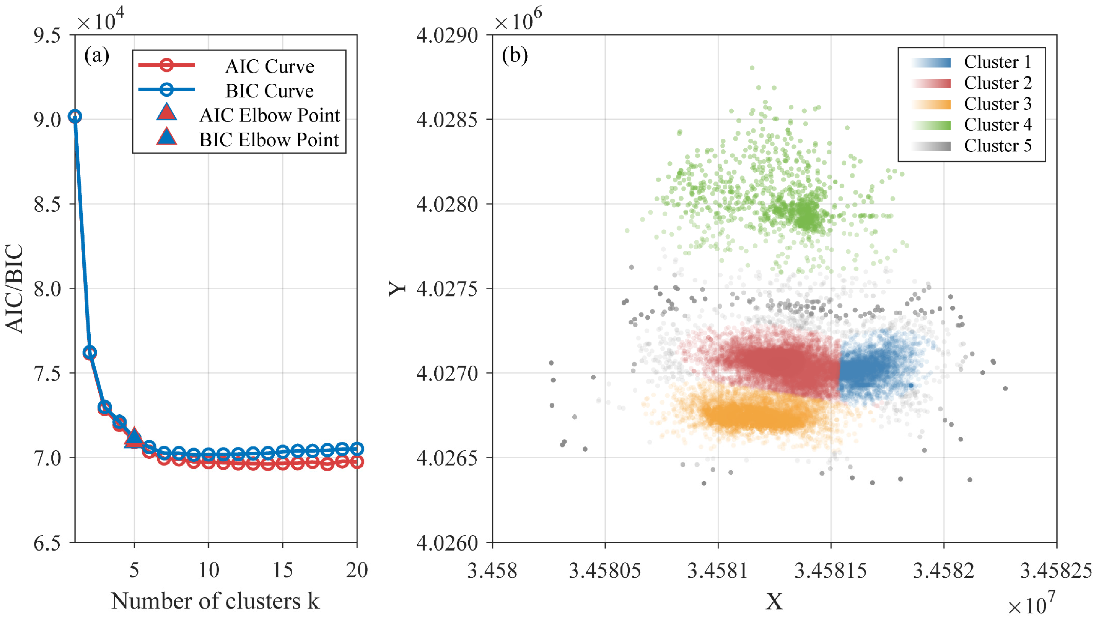
The optimal number of clusters for the GMM was determined by integrating the AIC, BIC, and the elbow method. As illustrated in Figure 4a, both AIC and BIC curves exhibit distinct inflection points at five clusters, establishing this as the optimal cluster count. Figure 4b visualizes the spatial clustering results of mining-induced seismicity events.
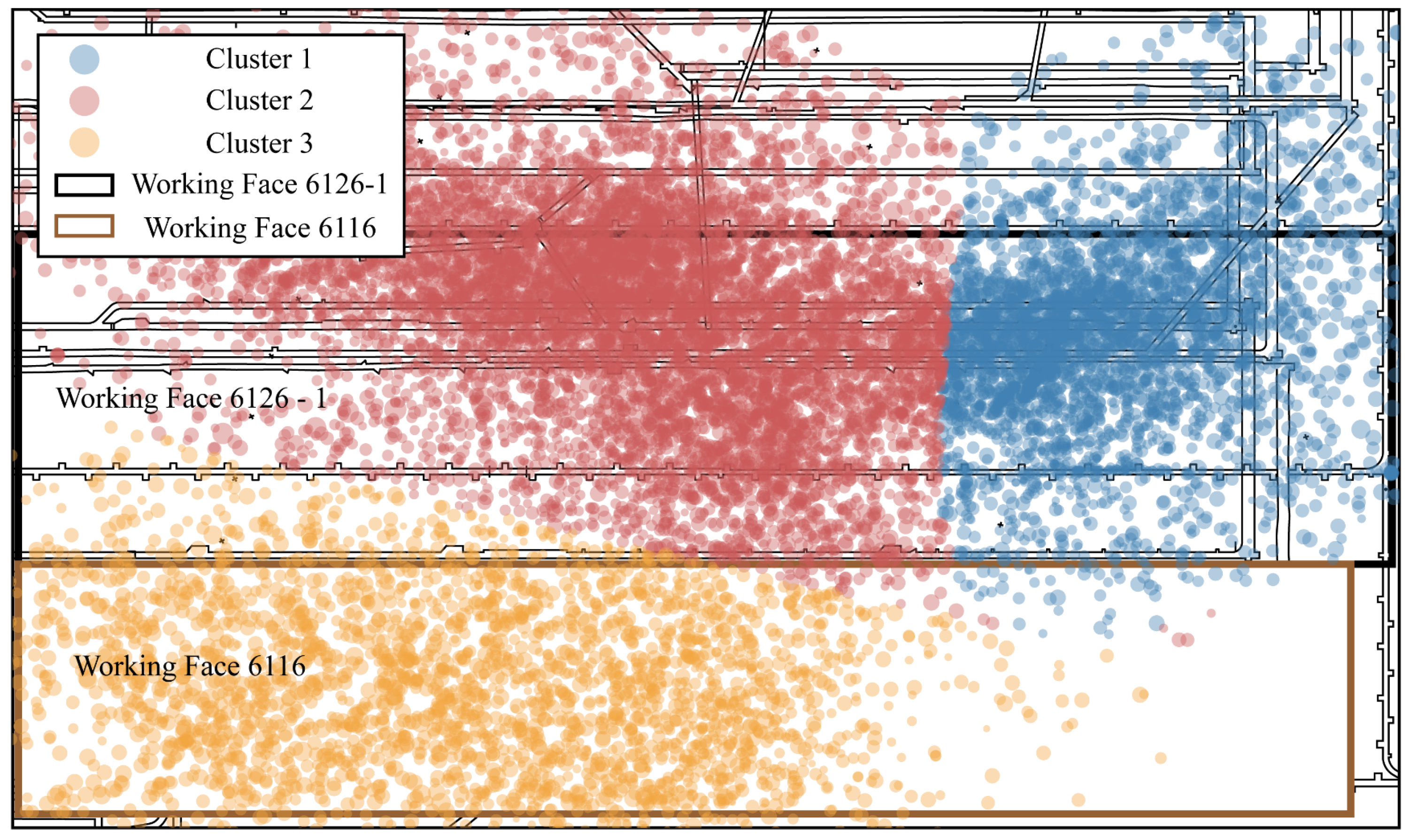
To ensure statistical reliability of b-value calculations—which requires more than 500 events above the minimum completeness magnitude for stable estimation—only three clusters containing more than 2000 events were retained for detailed analysis [34,35]. As illustrated in Figure 5, Cluster 1 and Cluster 2 are mainly distributed in the eastern and central parts of the working face 6126-1, respectively, while Cluster 3 is concentrated around the working face 6116 and its adjacent area. This spatial distribution demonstrates strong correspondence with actual mining layouts, validating the effectiveness of the clustering methodology in identifying seismotectonic domains.
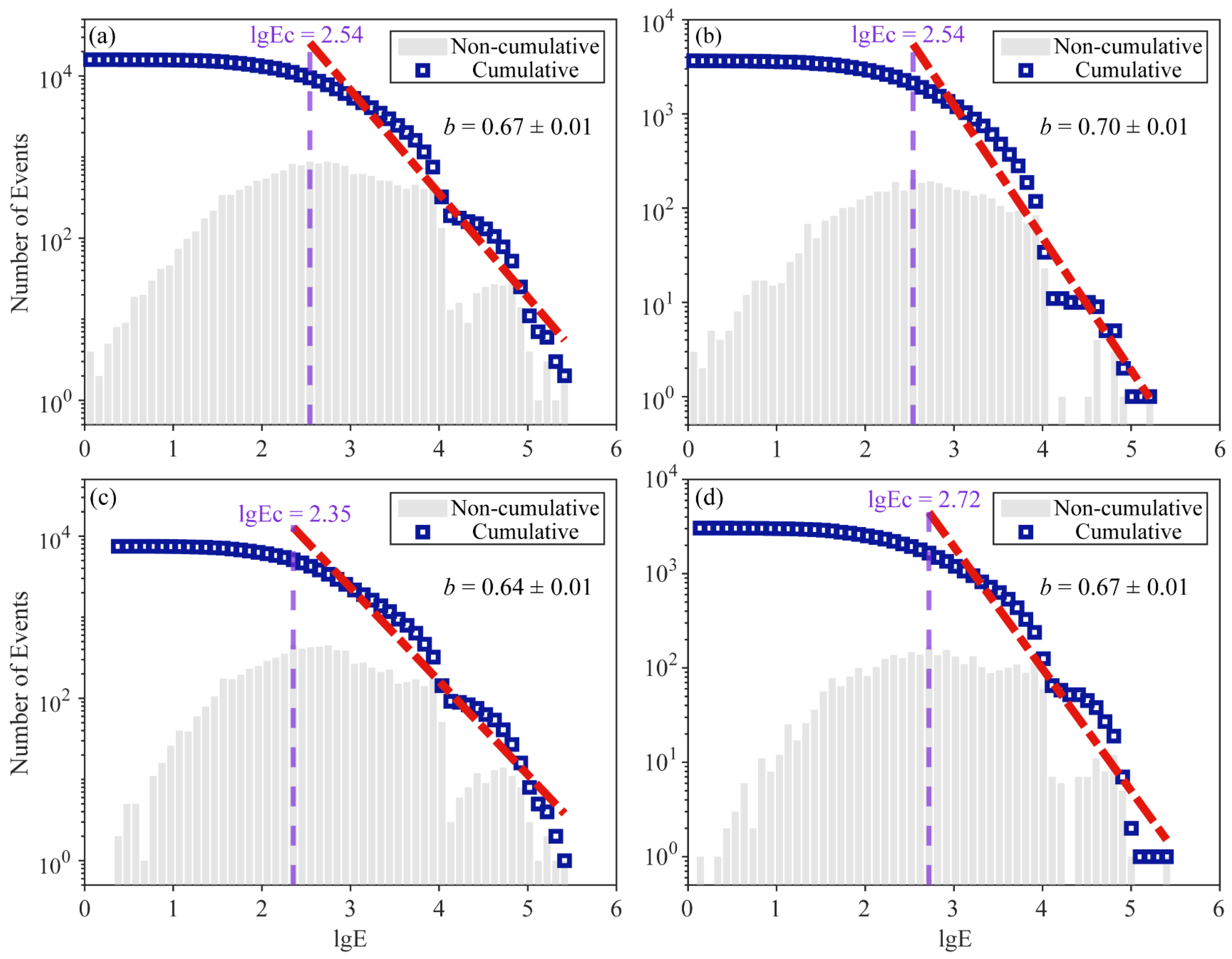
Frequency-energy distribution analysis was performed for the entire mine and three individual clusters using a logarithmic energy bin width of 0.1. The results are shown in Figure 6. For the full dataset, the completeness energy threshold was 2.54, and the b-value was estimated using maximum likelihood estimation as 0.67 ± 0.01 (Figure 6a).

3.2. Temporal Evolution of b-Values

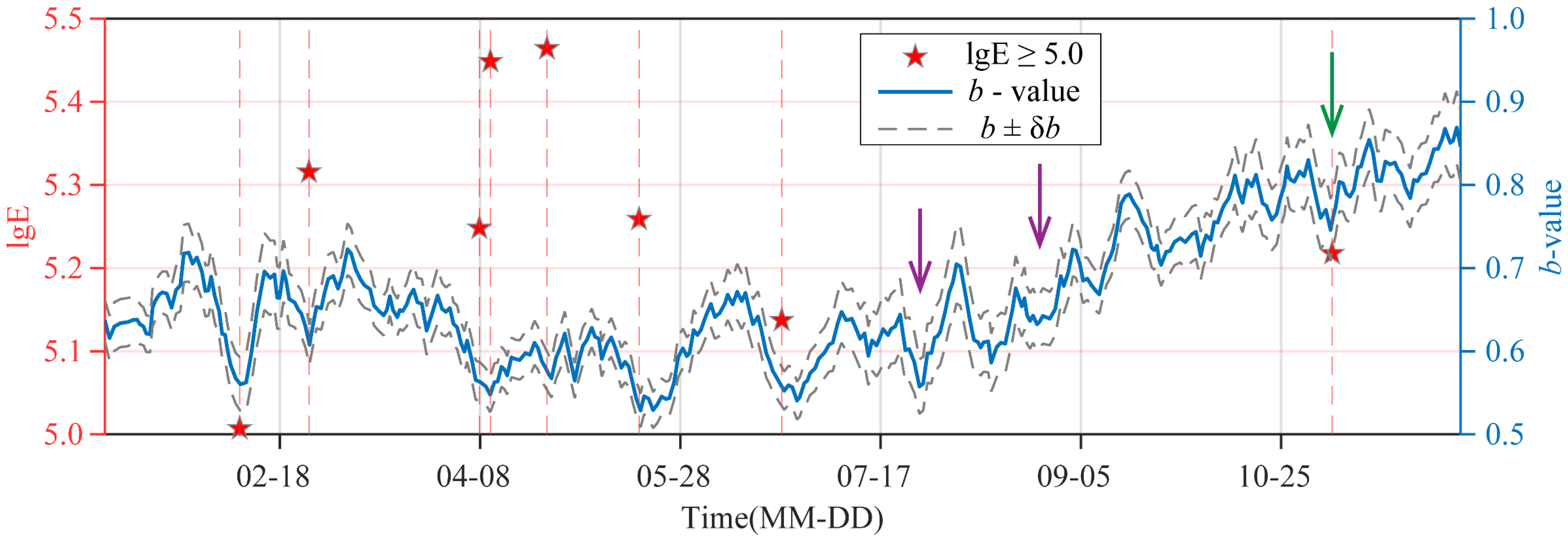
The temporal variation of the b-value was analyzed using a sliding time window method. A window width of 10 days and a step size of 1 day were selected, ensuring that each window contained more than 100 events. The resulting b-value time series is shown in Figure 7. During the study period, b-values ranged from 0.53 to 0.87, with an average of 0.67, displaying distinct phase characteristics.
The first half of 2024 exhibited the most pronounced fluctuations in b-values. This phase coincided with seven high-energy events (lgE > 5.0, E > 105 J), during which b-values remained persistently depressed—predominantly below 0.7—with a mean of 0.63. The initial high-energy event (February 7, lgE = 5.0) triggered an acute b-value drop to 0.56, followed by rapid recovery, reflecting a characteristic stress accumulation–release–adjustment cycle. From April to June, b-values sustained critically low levels (mean = 0.59), preceding six high-energy events. Each event was heralded by an accelerated b-value decline.
In the second half of 2024, the b-value exhibited a different evolution pattern, with smaller fluctuations and an overall increasing trend. After September, b-values were mostly above 0.7, except for a single high-energy event on November 6 (lgE = 5.2), during which the b-value temporarily dropped to 0.76. It is worth noting that statistical analysis shows that high-energy events predominantly occurred when the b-value fell below 0.6, aligning with local minima in the temporal profile. This recurrent pattern—b-value collapse, high-energy rupture, and subsequent recovery—vividly reflects the dynamic process of stress accumulation and release in the mine. It underscores the potential of b-value monitoring as a tool for seismic hazard assessment. A sustained b-value below 0.6 may serve as a practical threshold for elevated alert levels in a real-time microseismic early warning framework.

4. Discussion

4.1. Application of Clustering Analysis in b-Value Estimation

The frequency–magnitude relationship is a fundamental method for seismic hazard assessment, and its reliability depends on the homogeneity of the statistical sample. In small-scale areas such as mines, accurate reflection of regional stress conditions and the ratio of large to small events can only be achieved when the analyzed seismic events originate from the same structural system and the b-value remains statistically stable [36,37,38]. The spatial distribution of b-values can be used to infer the activity of associated fractures or faults—typically, a b-value greater than 1 indicates fracture expansion, while b-values less than 1 suggest fault activation [39,40,41]. Given the significant spatial clustering and temporal evolution of mining-induced seismicity, performing rational spatial clustering analysis is essential for understanding seismic mechanisms and quantifying seismic hazard risks in mining environments [42].
Conventional seismological studies often adopt hard clustering methods based on density, such as K-means [43] and DBSCAN [44], in which each data point is assigned to a single cluster. Novianti et al. used the K-means algorithm to cluster earthquake data in Indonesia from 1970 to 2015, revealing distinct patterns between shallow offshore and inland fault zone earthquakes [45]. Irwansyah and Winarko combined K-means with kriging interpolation to construct spatial zoning of seismic building damage [46]. Cesca developed the Seiscloud tool based on the DBSCAN algorithm, enabling automated clustering of large-scale earthquake catalogs [47]. However, such hard clustering methods are limited in handling the complexity and uncertainty of mining-induced seismic distributions.
In contrast, the GMM, as a probability-based soft clustering method, provides the probability of each event belonging to each cluster. Its covariance matrix captures the shape, size, and orientation of clusters, making it particularly suitable for modeling non-spherical and anisotropic spatial patterns commonly observed in mine seismicity. Wang et al. applied GMM to microseismic signals in the Baoji lead-zinc mine in Shaanxi, successfully distinguishing seismic events with different mechanisms [48]. This study leverages the soft clustering capability of GMM to effectively delineate spatially and genetically homogeneous seismic subregions.
It should be noted that the apparent sharp boundaries between the GMM clusters are not physical lines, but rather a visual effect caused by the high density of events within each cluster. This phenomenon arises from the inherent characteristics of the Gaussian Mixture Model, which performs soft clustering by assigning events to clusters based on their posterior probabilities. These boundaries should therefore be interpreted as probabilistic transition zones. To better illustrate this uncertainty, Figure 4 employs color transparency to reflect the probability of each event’s cluster membership.
As shown in Table 2, the analysis of cluster parameters reveals the seismic hazard characteristics across regions: although Cluster 2 contains the largest number of events (7474), it has the lowest b-value (0.64) and includes five strong events with energy greater than 105 J, indicating a high degree of stress concentration and significant large-event potential. In contrast, Cluster 1 shows a relatively higher b-value (0.70) and the lowest average energy (1437.79 J), representing a relatively lower-risk area. Cluster 3, while having fewer events (3041), shows the highest average energy (2575.94 J) and a higher completeness energy threshold (2.72), suggesting a greater tendency for sudden, high-energy seismic releases during rock failure.
By identifying spatially clustered regions with sufficient event counts using GMM, this approach ensures statistical robustness in b-value estimation and enables the b-value to reliably reflect inter-cluster differences in stress state. This integrated analysis—combining b-values, energy characteristics, and spatial clustering—provides an effective means for fine-scale identification of stress-concentrated zones and localized seismic risk assessment in mining areas.

4.2. Spatial Distribution Patterns of Mining-Induced Seismicity

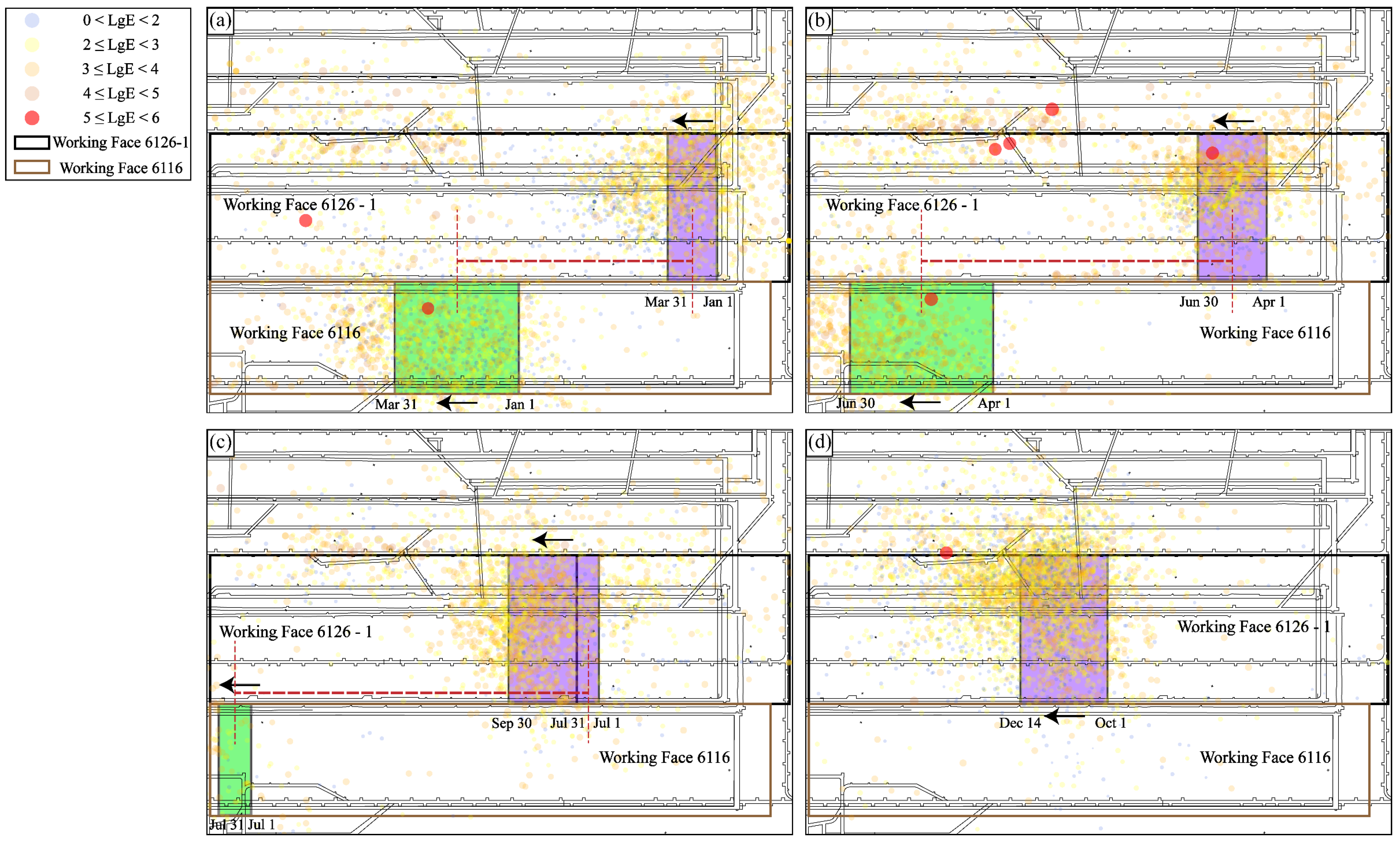
During 2024, mining operations primarily focused on the working face 6116 (active until 31 July) and working face 6126-1 (year-round extraction). Spatial seismicity distributions from the SOS microseismic monitoring system clearly demonstrate the causal relationship between excavation disturbances and seismic activity. As illustrated in Figure 8, seismicity migrated progressively with face advancement, confirming excavation as the dominant triggering mechanism.
During the first quarter (January to March; Figure 8a), seismic events were predominantly observed in the central region of the working face 6116 and the western sector of the working face 6126-1. Notably, high-energy events (lgE > 5.0) occurred near the return airway of the working face 6116 and at the forefront of the advancing face. Seismic events on the return air side were closely linked to the goaf area from the previously mined 6115 oil shale formation; mining-induced seismic events triggered coordinated movements of overlying strata above the goaf, leading to high-energy seismic events. Events ahead of the working face were attributed to rock fracturing due to elevated advance abutment pressure. From April to June (Figure 8b), the occurrence of high-energy seismic events notably increased, with most events still concentrated at the forefront of the working face 6126-1 and near the return air entry of the working face 6116. This suggests that excessive advance abutment pressure and stress concentration zones releasing energy abruptly are key mechanisms responsible for generating high-energy seismic events. During July to September (Figure 8c), seismic activity patterns shifted: due to the cessation of mining at the working face 6116, seismic events in that area significantly declined. The overall seismicity in the mine decreased, and no high-energy events were recorded. Seismic events were primarily concentrated along the advancing working face 6126-1, continuing to migrate forward with the mining progress. From October to December (Figure 8d), seismic frequency rose again, with epicenters mainly located in the central section of the working face 6126-1. This event’s location suggests it was likely triggered as working face 6126-1 advanced beneath a critical stress concentration zone associated with the boundary or a remnant pillar of the overlying 6115 goaf.
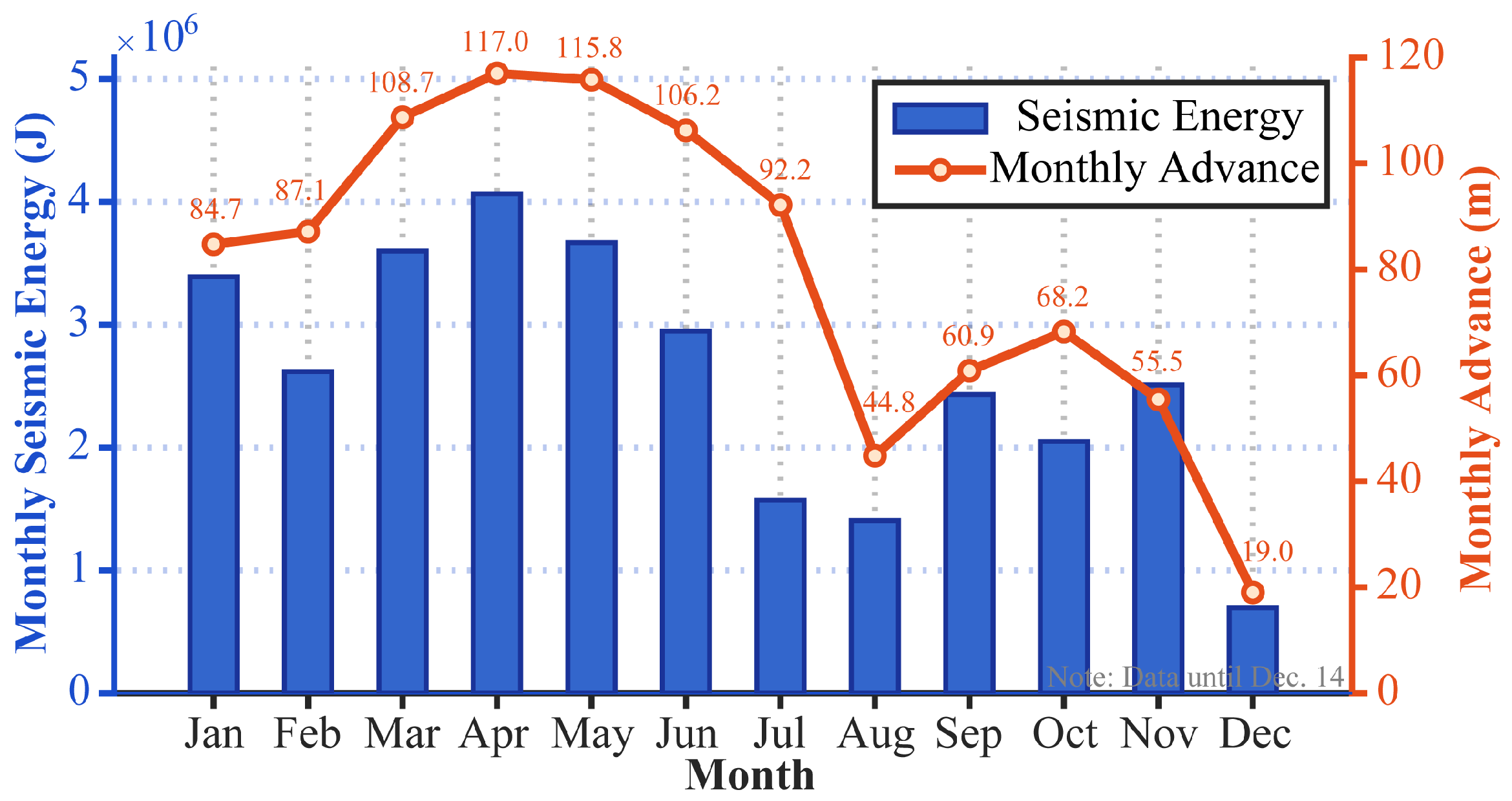
To quantitatively assess the relationship between mining intensity and seismic activity, Figure 9 compares the monthly mining advance with the monthly seismic energy release. The results reveal a significant positive correlation between the two variables, with their fluctuations largely synchronized—periods of intense mining correspond to increased seismic energy release, while periods of reduced mining activity show more stable seismic behavior. This finding holds important engineering implications: when elevated seismic risk is detected, appropriately reducing the mining advance rate can help mitigate stress accumulation, thereby lowering the likelihood of seismic events or rockbursts and ensuring operational safety. Overall, throughout the year 2024, the distribution of mining seismicity and mining activities showed a high degree of spatial-temporal correspondence, indicating that stress perturbations caused by the advancement of the working face directly control the stress state and fracture modes in the seismic source area, serving as the fundamental mechanism triggering mining seismic events.

4.3. Challenges in b-Value Interpretation and the Integrated Approach to Hazard Assessment

While the temporal evolution of the b-value is a widely recognized indicator for seismic hazard assessment, its interpretation is complex and requires consideration of the dynamic mining environment. The analysis demonstrates a strong overall correlation between b-value and high-energy events, yet a granular examination of specific periods reveals a nuanced interplay of factors.
A notable example is the period from mid-July to early September (marked by purple arrows in Figure 7), when persistently low b-values were recorded but no events with lgE > 5.0 occurred. This apparent anomaly reflects the statistical nature of the b-value: a low b-value correctly identifies a state of high regional stress, but the ultimate rupture requires a sufficient trigger. During this period, a profound change in the mine’s stress regime likely mitigated this triggering potential.
Primarily, overall mining intensity declined significantly. As shown in Figure 9, July and August recorded the lowest monthly advance rates during the entire monitoring period, primarily due to the cessation of mining at working face 6116 on 31 July. This reduction in excavation weakened the dominant source of dynamic perturbation, allowing accumulated stress to dissipate more gradually. Similar findings were reported by Wojtecki et al. [49], who demonstrated that seismic energy release strongly depends on mining progress, with reduced advance rates effectively suppressing the occurrence of high-energy seismic events.
Another factor is the gradual decoupling of stress interactions between adjacent working faces. Before July, concurrent extraction at working faces 6116 and 6126-1 likely created overlapping abutment pressure fields, amplifying stress concentrations and increasing the probability of high-energy events. After mining ceased at the working face 6116, the advancing working face 6126-1 progressively moved farther away, reducing the extent of overlapping stress fields. To illustrate this effect, red dashed lines were added in Figure 8 to schematically represent the increasing average staggered distance between the two working faces, indicating a progressive weakening of stress interference. Previous studies have shown that maintaining an appropriate staggered distance between working faces is critical for ensuring seismic stability [50,51]. Consequently, despite persistently low b-values indicating elevated inherited stresses, the reduction of stress interaction between working faces significantly decreased the likelihood of high-energy seismic events.
Conversely, the isolated high-energy event on November 6, which occurred during a period of relatively high regional b-value (Figure 7, green arrow), highlights the importance of localized, inherited stress concentrations. The concept of an advanced mining influence range posits that both static abutment stress and dynamic disturbances are superimposed ahead of the working face [51]. While the spatially-averaged b-value reflects the regional state of this influence, it can be overwhelmed by local anomalies. In this case, the event was triggered as the lower 6126-1 face advanced under the high-stress abutment zone formed by the remnant pillar of the overlying 6115 goaf. This observation aligns with research emphasizing the dominant role of local structural controls in triggering high-magnitude mining-induced seismicity.
In summary, the b-value remains a valuable proxy for tracking stress evolution but should not be used in isolation for seismic hazard assessment. A comprehensive and robust evaluation requires an integrated, multi-parameter framework that incorporates b-value analysis alongside detailed mining dynamics, spatial stress interactions, and localized geological conditions.

4.4. Limitations and Future Research Directions

A key methodological choice in this study was the direct use of lgE for b-value estimation, motivated by the desire to establish a more fundamental and physically grounded basis for seismic hazard assessment. Since the b-value critically depends on the consistency of the underlying scaling parameter, regardless of whether it is magnitude or energy, it is important to place this approach within the broader context of seismological scaling laws. There is an ongoing scientific debate surrounding the consistency and universal applicability of classical magnitude scales. For instance, while the Moment Magnitude (Mw) is the most widely used magnitude scale in seismology, its formulation relies on assumptions that may not hold universally. Recent work has indicated that the empirical basis for certain Mw relationships rests on equations with limited validity ranges, which can affect the consistency of magnitude estimates across regions [52]. Consequently, inconsistencies in the adopted magnitude scale can directly influence the resulting b-value estimates.
By employing seismic energy as a fundamental physical parameter that does not suffer from saturation issues, the present study circumvents these limitations and ensures an internally consistent framework for analyzing the mining-induced microseismicity dataset. However, a trade-off exists: direct comparisons between the energy-based b-value results and studies relying on conventional magnitude-based approaches become less straightforward. To bridge this gap, future research could incorporate parallel analyses by deriving magnitudes for the microseismic catalog using a more robust and globally consistent scale, such as the Das Magnitude scale (Mwg) proposed by Das et al. [53]. This would help validate whether the spatiotemporal patterns identified in this study are independent of the choice of scaling parameter, thereby further strengthening the proposed hazard assessment framework.

5. Conclusions

This study systematically deciphers the spatiotemporal evolution of mining-induced seismicity and its intrinsic linkage to excavation disturbances using enhanced G–R relationship and GMM clustering on 2024 microseismic data from a coal mine in Gansu Province, China. The results validate the applicability of G–R relationships in mining seismicity and develop a b-value dynamics-based hazard assessment framework. Key conclusions are as follows:
  • Spatial clustering effectively reveals the heterogeneous distribution of mining-induced seismic hazards. The GMM-based clustering divided the mining area into several regions with distinct stress states, each exhibiting significantly different b-values. Low b-value regions (e.g., Cluster 2 with a b-value of 0.64) indicate areas of high stress concentration and elevated potential for high-energy seismic events, while high b-value regions (e.g., Cluster 1 with a b-value of 0.70) suggest relatively uniform stress release and lower seismic risk. This refined b-value analysis based on clustering overcomes the limitations of uniform b-value estimation across the entire mine and provides a new approach for localized seismic hazard assessment.
  • The temporal evolution of b-values has clear early-warning implications for high-energy seismic events. Sliding window analysis shows that b-values fluctuate within the range of 0.53 to 0.87 in stages. When the b-value sharply dropped to 0.6 or below, the probability of high-energy seismic events significantly increases. Among the eight strong seismic events with lgE greater than 5.0 during the study period, seven occurred when the b-value was below 0.6, all located at troughs in the b-value curve. This cycle of “b-value decline—strong seismic event—b-value recovery” clearly reflects the dynamic process of stress accumulation and release in the mining area, serving as an important indicator for short-term seismic warnings.
  • Mining disturbance is the dominant factor driving mining-induced seismic activity. The spatial migration of seismic events closely follows the advancement of the working faces, and a strong positive correlation is observed between monthly mining progress and monthly seismic energy release. After the cessation of mining at the working face 6116, seismic activity in that area declined markedly, further confirming the controlling effect of mining operations. This understanding suggests that seismic hazard can be mitigated by optimizing mining intensity and advancing rates.
The proposed framework for seismic monitoring based on spatiotemporal b-value analysis holds significant engineering application value. In practice, this framework can be integrated with existing microseismic monitoring systems to enable real-time dynamic monitoring and early warning of seismic hazards by tracking local b-value variations and identifying high-risk clustered zones. Furthermore, adjusting mining intensity in response to b-value evolution provides an effective strategy to mitigate the occurrence of strong seismic events, thereby offering crucial technical support for safe and efficient deep coal mining.

Author Contributions

Conceptualization, H.W. and X.Y.; methodology, H.W. and X.Y.; software, H.W. and X.Y.; validation, H.W., X.Y. and J.W.; formal analysis, H.W.; investigation, H.W., X.Y., J.W. and X.L.; resources, H.W. and X.Y.; data curation, H.W. and X.Y.; writing—original draft preparation, H.W.; writing—review and editing, H.W., X.Y. and J.W.; visualization, H.W.; supervision, H.W. and X.Y.; project administration, H.W. and X.Y.; funding acquisition, X.Y. and J.W. All authors have read and agreed to the published version of the manuscript.

Funding

This research was funded by the National Natural Science Foundation of China, grant number 43271404; Natural Science Foundation of Gansu Province, China, grant number 25JRRA394; Science and Technology Program of Lanzhou, China, grant number 2025-2-84.

Institutional Review Board Statement

Not applicable.

Informed Consent Statement

Not applicable.

Data Availability Statement

The data presented in this study are not publicly available due to commercial confidentiality of the coal mine.

Acknowledgments

The authors are grateful to all people who help us with this paper.

Conflicts of Interest

The authors declare no conflicts of interest.

Abbreviations

The following abbreviations are used in this manuscript:
SOSSeismological Observation System
GMMGaussian Mixture Model
G–RGutenberg–Richter
EMExpectation-Maximization
AICAkaike Information Criterion
BICBayesian Information Criterion

References

  1. Hudyma, M.; Potvin, Y.H. An engineering approach to seismic risk management in hardrock mines. Rock Mech. Rock Eng. 2010, 43, 891–906. [Google Scholar] [CrossRef]
  2. Gibowicz, S.J. Seismicity induced by mining. In Advances in Geophysics; Elsevier: Amsterdam, The Netherlands, 1990; Volume 32, pp. 1–74. [Google Scholar]
  3. Gibowicz, S.J. Seismicity induced by mining: Recent research. Adv. Geophys. 2009, 51, 1–53. [Google Scholar]
  4. Zhu, J.-B.; Ma, B.-W.; Xie, H.-P.; Gao, F.; Zhou, H.-W.; Zhou, C.-T.; Zheng, F.-R. Differences and connections between mining seismicity and coal bursts in coal mines and preliminary study on coal bursts induced by mining seismicity. J. China Coal Soc. 2022, 47, 3396–3409. [Google Scholar]
  5. Ayad, A.; Bakkali, S. Economic impact of derangements on mining process—Case study: Sidi Chennane. J. Min. Environ. 2022, 13, 989–996. [Google Scholar]
  6. Dou, L.-M.; Chen, T.-J.; Gong, S.-Y.; He, H.; Zhang, S.-B. Rockburst hazard determination by using computed tomography technology in deep workface. Saf. Sci. 2012, 50, 736–740. [Google Scholar] [CrossRef]
  7. Ge, M. Efficient mine microseismic monitoring. Int. J. Coal Geol. 2005, 64, 44–56. [Google Scholar] [CrossRef]
  8. Yang, C.-X.; Luo, Z.-Q.; Hu, G.-B.; Liu, X.-M. Application of a microseismic monitoring system in deep mining. J. Univ. Sci. Technol. Beijing Miner. Metall. Mater. 2007, 14, 6–8. [Google Scholar] [CrossRef]
  9. Li, S.-J.; Feng, X.-T.; Li, Z.-H.; Chen, B.-R.; Zhang, C.-Q.; Zhou, H. In situ monitoring of rockburst nucleation and evolution in the deeply buried tunnels of Jinping II hydropower station. Eng. Geol. 2012, 137, 85–96. [Google Scholar] [CrossRef]
  10. Gutenberg, B.; Richter, C.F. Earthquake magnitude, intensity, energy, and acceleration. Bull. Seismol. Soc. Am. 1942, 32, 163–191. [Google Scholar] [CrossRef]
  11. Toda, S.; Stein, R.S.; Reasenberg, P.A.; Dieterich, J.H.; Yoshida, A. Stress transferred by the 1995 Mw = 6.9 Kobe, Japan, shock: Effect on aftershocks and future earthquake probabilities. J. Geophys. Res. Solid Earth 1998, 103, 24543–24565. [Google Scholar] [CrossRef]
  12. Wyss, M.; Sammis, C.G.; Nadeau, R.M.; Wiemer, S. Fractal dimension and b-value on creeping and locked patches of the San Andreas fault near Parkfield, California. Bull. Seismol. Soc. Am. 2004, 94, 410–421. [Google Scholar] [CrossRef]
  13. Urbancic, T.; Trifu, C.; Long, J.; Young, R. Space-time correlations of b values with stress release. Pure Appl. Geophys. 1992, 139, 449–462. [Google Scholar] [CrossRef]
  14. Boettcher, M.S.; McGarr, A.; Johnston, M. Extension of Gutenberg-Richter distribution to Mw −1.3, no lower limit in sight. Geophys. Res. Lett. 2009, 36, 1–5. [Google Scholar] [CrossRef]
  15. Ma, X.; Westman, E.; Slaker, B.; Thibodeau, D.; Counter, D. The b-value evolution of mining-induced seismicity and mainshock occurrences at hard-rock mines. Int. J. Rock Mech. Min. Sci. 2018, 104, 64–70. [Google Scholar] [CrossRef]
  16. Huang, L.; Zhao, A.-H.; Wu, Q.-J.; Xu, Z.-Y.; Pan, J.-T.; Zhang, F.-X.; Yao, Z.-X. Characteristics of seismic b-value of Changning shale gas region, Sichuan, from a dense seismic array. Acta Seismol. Sin. 2024, 46, 825–843. [Google Scholar]
  17. Wu, A.-X.; Wu, L.-C.; Liu, X.-H.; Wang, C.-L.; Huang, W.-S.; Zhu, Q.-J. Space-time distribution of microseismic activities in mines. Chin. J. Eng. 2012, 34, 609–613. [Google Scholar]
  18. Hudyma, M.R. Analysis and Interpretation of Clusters of Seismic Events in Mines; University of Western Australia Perth: Crawley, Australia, 2008. [Google Scholar]
  19. Cheng, J.-L. Cluster Analysis of Monitoring Data of Coal Mine Microseism. Master’s Thesis, China University of Mining and Technology, Xuzhou, China, 2020. [Google Scholar]
  20. Luo, F.-Z. Study on Mining Seismic Law of Protective Layeron Deep Giant Thick Coalbed Oil Shale. Master’s Thesis, China University of Mining and Technology, Xuzhou, China, 2023. [Google Scholar]
  21. Lv, C.-G.; Dou, L.-M.; He, J.; Shan, S.-P.; Liu, B.; Guo, X.-Q. Development and use of SOS microseismic monitoring system at Taoshan coal mine. China Coal 2010, 36, 86–90. [Google Scholar]
  22. Zhang, P. Research on Prediction Method of Mine Earthquake in Time SEQUENCE based on Clustering Analysis. Master’s Thesis, China University of Mining and Technology, Xuzhou, China, 2023. [Google Scholar]
  23. Yang, L. Study on the Early Warning of Rockburst Event of a Coal Mine in Hegang Mining Area Based on Mine Earthquake and Microseismic Monitoring. Master’s Thesis, Institute of Engineering Mechanics, China Earthquake Administration, Harbin, China, 2022. [Google Scholar]
  24. Dempster, A.P.; Laird, N.M.; Rubin, D.B. Maximum likelihood from incomplete data via the EM algorithm. J. R. Stat. Soc. Ser. B (Methodol.) 1977, 39, 1–22. [Google Scholar] [CrossRef]
  25. Akaike, H. A new look at the statistical model identification. IEEE Trans. Autom. Control 2003, 19, 716–723. [Google Scholar] [CrossRef]
  26. Schwarz, G. Estimating the dimension of a model. Ann. Stat. 1978, 6, 461–464. [Google Scholar] [CrossRef]
  27. Kanamori, H. The energy release in great earthquakes. J. Geophys. Res. 1977, 82, 2981–2987. [Google Scholar] [CrossRef]
  28. Iwata, T. Estimation of completeness magnitude considering daily variation in earthquake detection capability. Geophys. J. Int. 2013, 194, 1909–1919. [Google Scholar] [CrossRef]
  29. Shi, X.-Y.; Wang, X.-Q.; Qiu, Y.-R.; Yuan, X.-X. Analysis of the minimum magnitude of completeness for earthquake catalog in China Seismic Experimental Site. Chin. J. Geophys. 2020, 63, 3683–3697. [Google Scholar]
  30. Wen, S.-L.; Liu, X.-Z.; Qin, M.-Z.; Liu, B.-Y.; Kang, B.-L.; Wu, B.-C. Completeness of the earthquake catalog of the 2023 Jishishan MS6.2 earthquake in Gansu Province. China Earthq. Eng. J. 2024, 46, 924–931. [Google Scholar]
  31. Woessner, J.; Wiemer, S. Assessing the quality of earthquake catalogues: Estimating the magnitude of completeness and its uncertainty. Bull. Seismol. Soc. Am. 2005, 95, 684–698. [Google Scholar] [CrossRef]
  32. Aki, K. Maximum likelihood estimate of b in the formula log N= a-bM and its confidence limits. Bull. Earthq. Res. Inst. Tokyo Univ. 1965, 43, 237–239. [Google Scholar]
  33. Shi, Y.-L.; Bolt, B.A. The standard error of the magnitude-frequency b value. Bull. Seismol. Soc. Am. 1982, 72, 1677–1687. [Google Scholar] [CrossRef]
  34. Nava, F.; Márquez-Ramírez, V.; Zúñiga, F.; Ávila-Barrientos, L.; Quinteros, C. Gutenberg-Richter b-value maximum likelihood estimation and sample size. J. Seismol. 2017, 21, 127–135. [Google Scholar] [CrossRef]
  35. Aiken, C.; Meng, X.; Hardebeck, J. Testing for the ‘predictability’of dynamically triggered earthquakes in The Geysers geothermal field. Earth Planet. Sci. Lett. 2018, 486, 129–140. [Google Scholar] [CrossRef]
  36. Rundle, J.B.; Turcotte, D.L.; Shcherbakov, R.; Klein, W.; Sammis, C. Statistical physics approach to understanding the multiscale dynamics of earthquake fault systems. Rev. Geophys. 2003, 41, 1–30. [Google Scholar] [CrossRef]
  37. Huang, Q.-H. Seismicity changes prior to the Ms8. 0 Wenchuan earthquake in Sichuan, China. Geophys. Res. Lett. 2008, 35, 1–5. [Google Scholar] [CrossRef]
  38. Wen, X.-Z.; Ma, S.-L.; Xu, X.-W.; He, Y.-N. Historical pattern and behavior of earthquake ruptures along the eastern boundary of the Sichuan-Yunnan faulted-block, southwestern China. Phys. Earth Planet. Inter. 2008, 168, 16–36. [Google Scholar] [CrossRef]
  39. Mousavi, S.M.; Ogwari, P.O.; Horton, S.P.; Langston, C.A. Spatio-temporal evolution of frequency-magnitude distribution and seismogenic index during initiation of induced seismicity at Guy-Greenbrier, Arkansas. Phys. Earth Planet. Inter. 2017, 267, 53–66. [Google Scholar] [CrossRef]
  40. Maity, D.; Ciezobka, J. Using microseismic frequency-magnitude distributions from hydraulic fracturing as an incremental tool for fracture completion diagnostics. J. Pet. Sci. Eng. 2019, 176, 1135–1151. [Google Scholar] [CrossRef]
  41. Zorn, E.; Kumar, A.; Harbert, W.; Hammack, R. Geomechanical analysis of microseismicity in an organic shale: A West Virginia Marcellus Shale example. Interpretation 2019, 7, T231–T239. [Google Scholar] [CrossRef]
  42. Woodward, K.; Wesseloo, J.; Potvin, Y. A spatially focused clustering methodology for mining seismicity. Eng. Geol. 2018, 232, 104–113. [Google Scholar] [CrossRef]
  43. MacQueen, J. Some methods for classification and analysis of multivariate observations. In Proceedings of the Fifth Berkeley Symposium on Mathematical Statistics and Probability; University of California Press: Oakland, CA, USA, 1967; Volume 1, pp. 281–298. [Google Scholar]
  44. Ester, M.; Kriegel, H.-P.; Sander, J.; Xu, X. A density-based algorithm for discovering clusters in large spatial databases with noise. In Proceedings of the KDD; AAAI Press: Menlo Park, CA, USA, 1996; pp. 226–231. [Google Scholar]
  45. Novianti, P.; Setyorini, D.; Rafflesia, U. K-Means cluster analysis in earthquake epicenter clustering. Int. J. Adv. Intell. Inform. 2017, 3, 81–89. [Google Scholar] [CrossRef]
  46. Irwansyah, E.; Winarko, E. Spatial data clustering and zonation of earthquake building damage hazard area. EPJ Web Conf. 2014, 68, 00005. [Google Scholar] [CrossRef]
  47. Cesca, S. Seiscloud, a tool for density-based seismicity clustering and visualization. J. Seismol. 2020, 24, 443–457. [Google Scholar] [CrossRef]
  48. Wang, J.; Zuo, Y.-Y.; Dong, L.-J.; Yan, X.-H. Spatiotemporal clustering of microseismic signals in mining areas: A case study of the Baoji lead-zinc mine in Shaanxi, China. Eng. Geol. 2025, 352, 108057. [Google Scholar] [CrossRef]
  49. Wojtecki, Ł.; Pakosz, R.; Apel, D.B.; Mendecki, M.J. Variability and Trends in Selected Seismological Parameters During Longwall Mining of a Coal Seam Disrupted by a Rockburst. Appl. Sci. 2025, 15, 8897. [Google Scholar] [CrossRef]
  50. Ma, S.-L.; Zhang, M.-W.; Ma, L.; Tian, Z.-C.; Li, X.; Su, Z.-H. Numerical simulation study on the evolution characteristics of the stress induced by mining in deep adjacent working faces. Geoenviron. Disasters 2023, 10, 17. [Google Scholar] [CrossRef]
  51. Zhou, K.-Y.; Deng, Z.; Kan, J.-L.; Dou, L.-M.; Li, J.-Z.; Duan, M.-K.; Kong, P. Determination of the advanced mining influence range in coal mines based on the statistical analysis of mining-induced seismicity. Appl. Sci. 2024, 14, 7737. [Google Scholar] [CrossRef]
  52. Das, R.; Das, A. Limitations of Mw and M Scales: Compelling evidence advocating for the das magnitude scale (Mwg)—A critical review and analysis. Indian Geotech. J. 2025, 1–19. [Google Scholar] [CrossRef]
  53. Das, R.; Sharma, M.L.; Wason, H.R.; Choudhury, D.; Gonzalez, G. A seismic moment magnitude scale. Bull. Seismol. Soc. Am. 2019, 109, 1542–1555. [Google Scholar] [CrossRef]
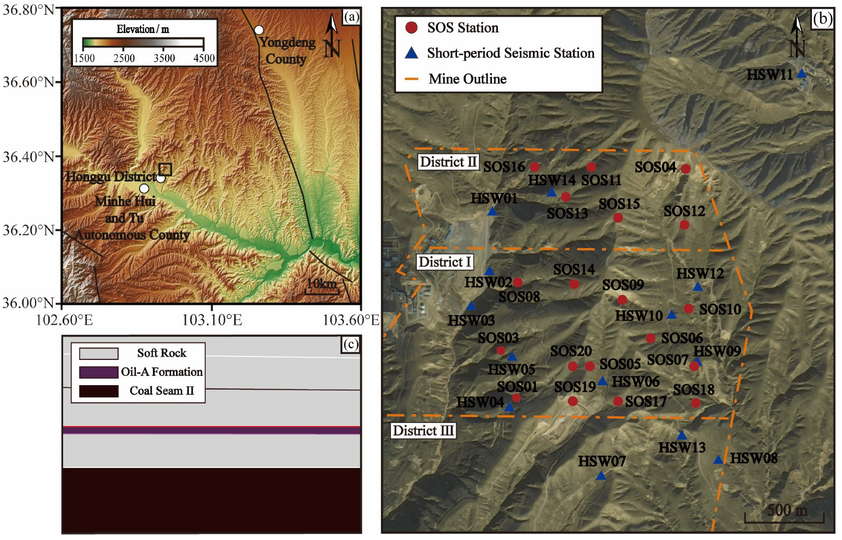
Figure 1. Location, geological setting, and monitoring layout of the study area. (a) Topographic map of the region surrounding the coal mine; the area within the black rectangle is magnified in (b). (b) Satellite imagery showing the detailed layout of the study area, including the mine outline and the distribution of microseismic stations. (c) Simplified stratigraphic column of the key geological strata in the mining area.
Applsci 15 10073 g001
Figure 2. Composition of the SOS Seismic Monitoring System. (a) DLM2001 Geophone. (b) Server. (c) Processing software.
Applsci 15 10073 g002
Figure 3. Statistical analysis of mine-induced seismic events. (a) Temporal distribution of seismic energy, where the blue lines represent events with energy greater than 105 J, and the gray lines indicate events with energy less than 105 J. (b) Histogram of monthly event counts. (c) Cumulative frequency curve of seismic events.
Applsci 15 10073 g003
Figure 4. GMM clustering analysis and results. (a) Determination of the optimal number of clusters k using AIC and BIC. The triangle symbols indicate the elbow points used for model selection. (b) Spatial distribution of the resulting GMM clusters. Each color represents a distinct cluster, and the color transparency of each event is proportional to its GMM assignment probability.
Applsci 15 10073 g004
Figure 5. Spatial distribution of clustered microseismic events within the working faces. The base map shows part of the mine structure. Bold colored outlines represent the two different working faces, and different colors represent microseismic events from different clusters.
Applsci 15 10073 g005
Figure 6. Frequency-energy distribution curves. (a) Full mine area; (b) Cluster 1; (c) Cluster 2; (d) Cluster 3. The gray bars represent non-cumulative frequencies, and the blue squares denote cumulative frequencies. The purple dashed line indicates the starting point for b-value estimation, and the red line represents the frequency–energy fitting.
Applsci 15 10073 g006
Figure 7. b-value and logarithmic energy time series. Left vertical axis (red): logarithmic energy (lgE). Right vertical axis (blue): b-values. Red stars: High-energy events (lgE > 5.0, E > 105 J). Blue solid line: b-value time series. Gray dashed lines indicate the standard error range of the b-value.
Applsci 15 10073 g007
Figure 8. Spatiotemporal evolution of mining-induced seismicity relative to excavation progress. The base map shows the mine layout, with bold black frames indicating working face areas. Colors denote the logarithmic energy of seismic events. The purple and green shaded rectangles denote the mined areas of the working faces 6126-1 and 6116, respectively, during each period. Black arrows indicate the mining direction. (a) 1 January–31 March 2024; (b) 1 April–30 June 2024; (c) 1 July–30 September 2024; (d) 1 October–14 December 2024.
Applsci 15 10073 g008
Figure 9. Correlation between monthly advance rates and cumulative seismic energy release. The blue bars represent the total seismic energy released each month, while the orange line indicates the monthly mining advance.
Applsci 15 10073 g009
Table 1. Summary of microseismic event energy distribution.
Energy Range (J)Number of EventsPercentage (%)
<1011821.15
101–102273217.20
102–103775048.79
103–104501031.54
104–1052021.27
>10580.05
Table 2. Clustering parameters and hazard indicators across seismic zones.
ClusterNumber of Eventsb-ValuelgECAverage Energy (J)Events > 105 J
Entire mine15,8840.672.541948.458
136600.702.541437.791
274740.642.351859.835
330410.672.722575.942
Disclaimer/Publisher’s Note: The statements, opinions and data contained in all publications are solely those of the individual author(s) and contributor(s) and not of MDPI and/or the editor(s). MDPI and/or the editor(s) disclaim responsibility for any injury to people or property resulting from any ideas, methods, instructions or products referred to in the content.