A Bi-Directional Coupling Calibration Model and Adaptive Calibration Algorithm for a Redundant Serial Robot with Highly Elastic Joints

Featured Application

The calibration method proposed in this paper is applicable to redundant robot arms with highly elastic joints. Such robot arms can be used in flexible product manufacturing scenarios, such as folding, packaging, and moving medical pads and diapers.

Abstract

This paper proposes a calibration method for redundant robot arms with highly elastic joints. The method uses the second-order Chebyshev polynomial to characterize the variation in the error with the poses of all joints. This error model is consistent with the variation in the gravitational torque on each joint and demonstrates good generalization. Based on this, the calibration model includes both kinematic errors and non-kinematic errors. For this high-dimensional model, an adaptive iterative identification algorithm is proposed for a large number of small error parameters of various types. The algorithm sets specific iteration rules for different types of error parameters and adjusts the convergence amplitude in each iteration, ensuring that the iterative algorithm converges to the global optimum. The simulation results show that for a redundant robot arm with 12 highly elastic joints, even with large linearization modeling errors, the new identification algorithm can gradually eliminate them during iteration, achieving an identification accuracy higher than 99.975% for all of the error parameters. The experimental results indicate that on a redundant robot arm with eight cable-driven elastic joints, the new model and identification algorithm reduce the 96.6% absolute positioning errors of the robot arm, enabling it to perform precise and flexible operations. It takes 40.534 s and 29.077 s to run the identification algorithm on MATLAB (R2023b, 2.10 GHz CPU) in the simulation and experiment, respectively.

1. Introduction

The absolute positioning accuracy is crucial to the working performance of robot arms [1]. For industrial robot arms, kinematic parameter errors are the main cause of absolute positioning errors, which mainly originate from the errors introduced during the manufacturing, assembly, and transmission processes of the links and joints [1,2]. Traditional calibration methods can effectively compensate for kinematic parameter errors and improve the absolute positioning accuracy of industrial robot arms, thus meeting the requirements of most tasks [1,2]. However, due to their strong rigidity, long links, and limited degrees of freedom, industrial robot arms are not suitable for some tasks in unstructured spaces that require flexible contact with soft workpieces, like diapers and medical pads [3]. As a result, redundant robot arms with highly elastic joints, short links, and a large number of joints have emerged [4,5,6].

Most conventional calibration methods fail to account for the influence of the robot arm’s self-weight and external payload on joint angle errors during calibration. For instance, the model presented by Jiang et al. [7,8,9] relies solely on fixed kinematic parameters. Likewise, Li et al. [10], Chen et al. [11], and Yang et al. [12] applied the product of exponentials (POE) theory to formulate a calibration framework; nevertheless, all kinematic parameters in their approach still remained constant.

Apart from the research previously discussed, other research has also been conducted on the compliance properties of robotic joints. A number of publications have introduced calibration methods for non-kinematic parameters using mass distribution information about the links. For instance, Klimchik et al. [13] and Nubiola et al. [14,15,16] proposed enhanced models incorporating both kinematic and non-kinematic parameters. Gong et al. [17] formulated non-kinematic parameters in terms of gravitational and center-of-mass variables—which are often impractical to measure directly—thereby eliminating the necessity of identifying these challenging quantities explicitly. Other efforts have targeted non-kinematic parameters resulting from external loads. Chen and Kao [18], for example, created a comprehensive stiffness model that translates joint space to Cartesian space, using techniques such as the conservative congruence transformation (CCT), to support calibration in the presence of external loads. Dumas et al. [19] refined the model into a more streamlined form, allowing for simplified stiffness calibration while largely preserving precision. Zhou et al. [20] broadened the framework to include both geometric inaccuracies and non-kinematic parameters. To enhance identifiability in real-world settings, Mamedov et al. [21] proposed a group of simplified models derived from parameter scaling and noise impact assessments. Theissen et al. [22] also presented an innovative calibration technique that integrates external loads with diverse directions and magnitudes. Assuming known gravitational and mass properties for each link, Nubiola and Bonev [23] suggested another stiffness model. Furthermore, Du et al. [24] and Chen et al. [25] established functional mappings relating two categories of non-kinematic parameters to end-effector positioning inaccuracies.

Based on the calibration models above, there are relatively few studies on parameter identification. The main method used is iterative identification without weight variation. That is, the error parameters identified in the previous round are compensated into the calibration model, and then the error parameters for the next round are solved. This process continues until the error parameters identified in a certain round are below the set threshold. Finally, the identification results of each round are accumulated to obtain the final error parameter results [11,23,26]. Some scholars have also proposed identification algorithms based on the Levenberg–Marquardt algorithm, which can adaptively adjust the damping factor in each iteration. This factor is multiplied by the identity matrix and then added to the Jacobian matrix of the least squares method to ensure that the matrix remains positive definite in each iteration [27].

These elasto-geometrical coupling modeling methods have the following four issues: (1) Calibration models are designed for industrial robot arms with high assembly precision, strong rigidity, and fewer degrees of freedom. The angular parameter errors and non-kinematic parameter values contained in these models are small, and the model dimensions are low. Therefore, the linearization errors introduced during modeling are small, and the models are well-conditioned. Simple iterative algorithms can achieve high-precision identification results. However, when dealing with large linearization errors and high-dimensional models, these methods are prone to divergence and are not suitable for redundant robot arms with lower assembly precision, higher flexibility, and more degrees of freedom. (2) Calibration models treat non-kinematic parameters and the influence of gravity as independent quantities to be identified and rely on simple geometric relationships to establish mappings from these parameters to joint angle errors. As a result, they are only applicable to typical industrial robot arms with two long links and two adjacent parallel joints. When applied to redundant robot arms with consistent link lengths, a large number of joints, and adjacent joints that are perpendicular to each other, the above mappings become highly nonlinear, making it difficult to linearize the calibration model. (3) The calibration models that adopted polynomials to model non-kinematic parameters only considered the pose impact of distal joints on the target joint, ignoring the impact of proximal ones. This strategy was effective on the industrial robot with only six joints but not applicable to the hyper-redundant one. In addition, most of these polynomials were constructed with high order or in a form (e.g., a series of trigonometric functions) that was difficult to map linearly, which probably resulted in ill-conditioned calibration models. (4) The identification algorithms currently used in robotic arm calibration are only suitable for low-dimensional calibration models. When facing high-dimensional ones, due to the large number and variety of error parameters, and the significant differences in linearization errors, the relatively simple and uniform iteration strategies of traditional identification algorithms find it difficult to converge the iterations to high-precision results. In summary, existing calibration methods are no longer sufficient for the calibration needs of elasto-geometrical coupling redundant robot arms. There is an urgent need for improvements in the completeness of parameter errors, the generalization of calibration models, and the convergence of identification algorithms.

To this end, this paper has three contributions: (1) The functional relationship between the joint angle errors and all joint angles is constructed based on Chebyshev polynomials during the modeling phase, thereby characterizing the flexible characteristics of the robot arm’s joints. (2) An elasto-geometrical coupling calibration model is established, which integrates kinematic parameter errors and non-kinematic errors, enhancing the completeness and generalization of the model. (3) With the aim of gradually reducing the impact of linearization errors, specific iteration rules are established for each type of parameter and integrated into a single iterative identification algorithm.

The remainder of this paper is organized as follows. Section 2 establishes the elasto-geometrical error model. Based on this, Section 3 establishes the calibration model. Section 4 proposes the iterative identification algorithm. Section 5 performs a simulation to validate the convergence of the identification algorithm and the accuracy of the identification results on an elastic robot arm with 12 joints. 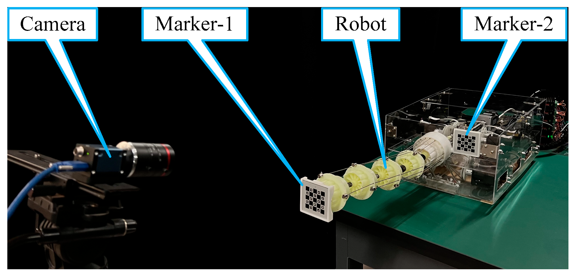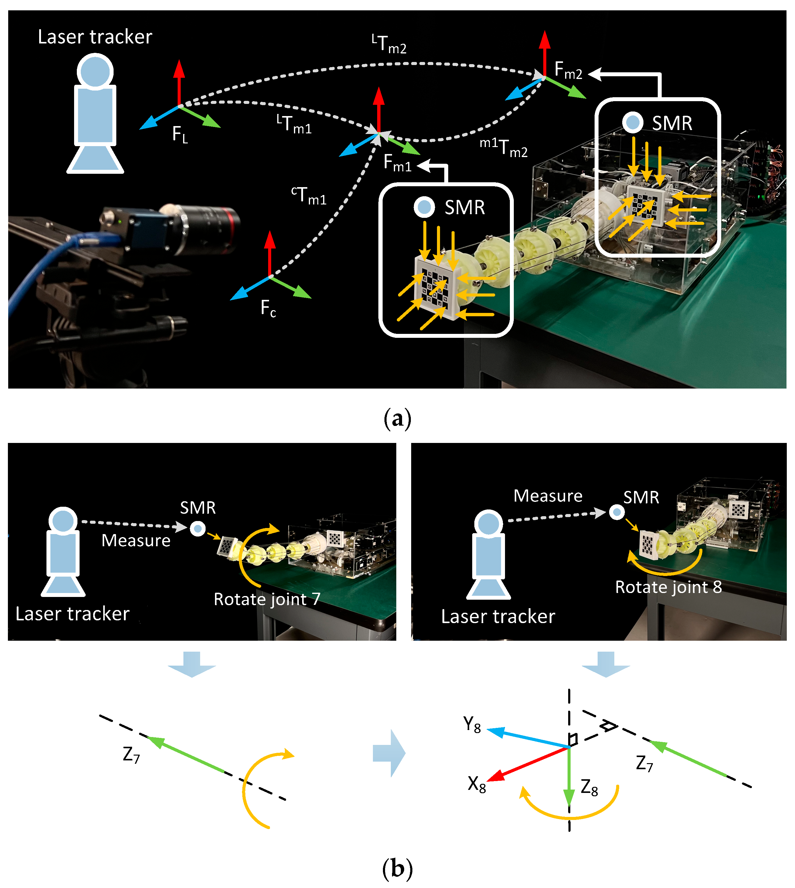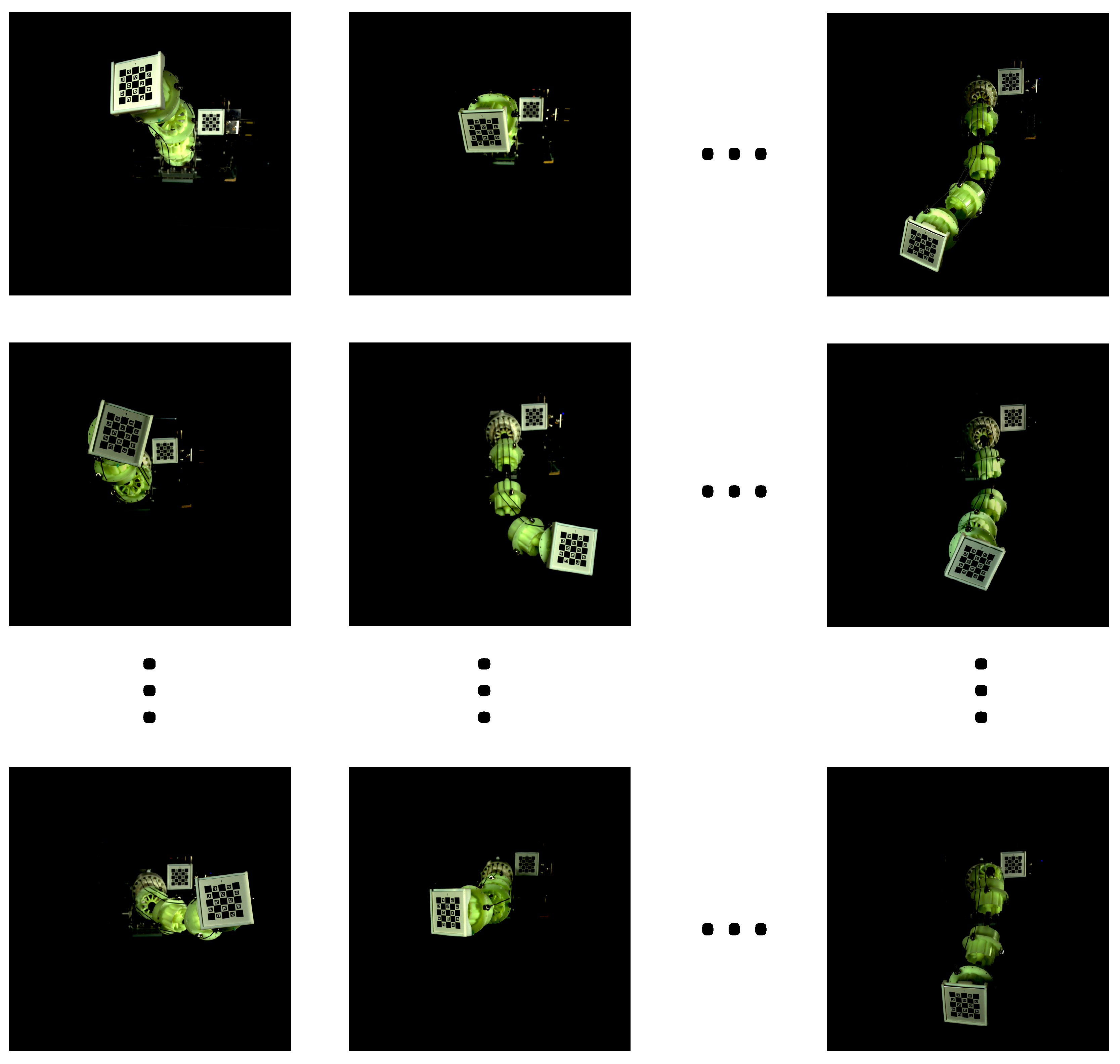Section 6 performs an experiment on a cable-driven robot arm with eight joints to demonstrate the accuracy of this new calibration model and the effectiveness of the identification algorithm. Section 7 draws conclusions.

2. Bi-Directional Coupling Elasto-Geometrical Error Model

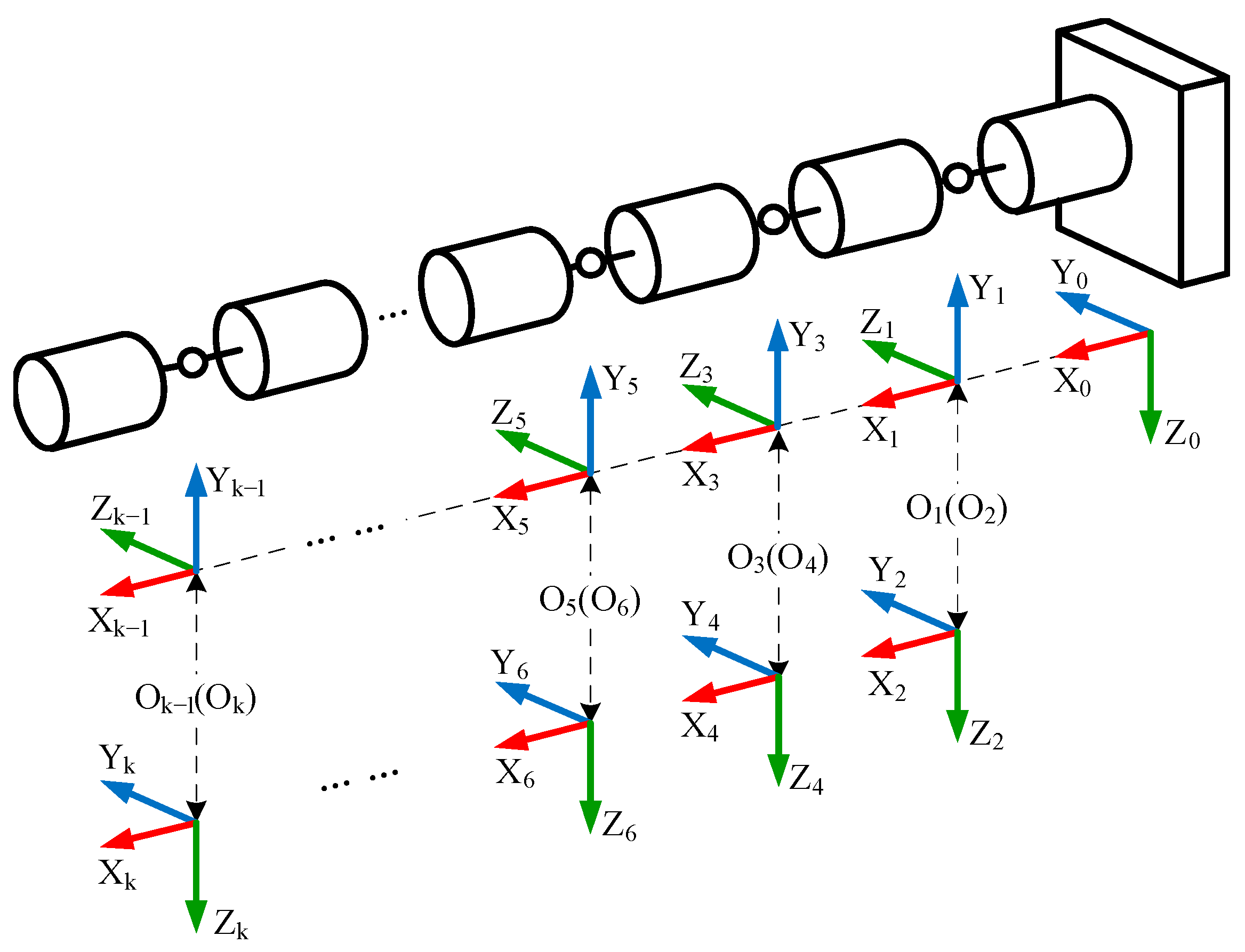
As shown in Figure 1, the coordinate systems of each joint of a serial redundant robot arm with k degrees of freedom (revolute joints) are established based on the Modified Denavit–Hartenberg (MDH) convention, namely the base coordinate system F₀ of the redundant robot arm and the joint coordinate systems F_i (i = 1, 2, …, k).

Let ⁱ⁻¹T_i denote the transformation matrix from the frame F_i−1 to F_i. Based on the MDH convention, the forward kinematic model of the i-th joint of the redundant robot arm is given by the following:

$${}^{0}T_i={}^{0}T_1{}^{1}T_2\dots {}^{i-1}T_i$$

(1)

Let R_x(α_i) and R_z(θ_i) denote the transformation matrices for rotations about the X-axis and Z-axis of the joint coordinate system, respectively. Let D_x(a_i) and D_z(d_i) denote the transformation matrices for translations along the X-axis and Z-axis of the joint coordinate system, respectively. α_i, a_i, θ_i, and d_i are the nominal MDH parameters for joint i, where α_i, a_i, and d_i are fixed values related to the structure, and θ_i is the joint angle command corresponding to the i-th joint in the j-th measurement configuration. Then, ⁱ⁻¹T_i in Equation (1) is calculated by

$${}^{i-1}T_i=R_x({\alpha }_i)D_x(a_i)R_z({\theta }_i)D_z(d_i).$$

(2)

The MDH parameter errors for the i-th joint can be represented as Δu_i = [δα_i, δa_i, δθ_i, δd_i]^T. Let Sθ_i and Cθ_i denote sin(θ_i) and cos(θ_i), respectively.

The redundant robot arm has a long and flexible arm structure, with a lower load-bearing capacity compared to industrial robot arms. It is not suitable for tasks such as machining that involve large loads and variable force directions. Instead, it is well-suited for tasks like detection, welding, and light-load assembly. Therefore, the primary source of flexibility errors is the additional bending of the elastic joints caused by the self-weight of the arm (including the end-effector), which affects the joint angle θ_i. First, the posture of the arm determines the lever arm of the gravitational moment acting on the axis of the target joint i. Thus, the joint angle error δθ_i caused by gravity should be represented as a function of all joint angles {θ₁, …, θ_k}. Let ${\widehat{\theta }}_i$ (i = 1, 2, …, k) denote the normalized joint angle values and θ_i(min) and θ_i(max) represent the minimum and maximum values of θ_i, respectively, which are determined by the joint angle limits of the robot arm. Then, this yields

$${\widehat{\theta }}_i={\displaystyle \frac{2[{\theta }_i-{\theta }_{i(\min )}]}{{\theta }_{i(\max )}-{\theta }_{i(\min )}}}-1.$$

(3)

Let the set {ⁱξ₍₀₎, ⁱξ₁₍₁₎, ⁱξ_i(2), …, ⁱξ_k(1), ⁱξ_k(2)} (where i = 1, 2, …, k) represent the polynomial coefficients, defined as the non-kinematic parameters here. Based on this, a combination of second-order Chebyshev polynomials is used to represent δθ_i as

$$\begin{array}{l}\delta {\theta }_i={}^i\xi _{(0)}+{}^i\xi _{1(1)}{\widehat{\theta }}_1+{}^i\xi _{1(2)}(2{\widehat{\theta }}_1^2-1)\\ +{}^i\xi _{2(1)}{\widehat{\theta }}_2+{}^i\xi _{2(2)}(2{\widehat{\theta }}_2^2-1)+\dots \\ +{}^i\xi _{k(1)}{\widehat{\theta }}_k+{}^i\xi _{k(2)}(2{\widehat{\theta }}_k^2-1)\end{array}$$

(4)

It should be noted that the second-order Chebyshev polynomial should originally include 0th-order, 1st-order, and 2nd-order terms. However, in Equation (4), all 0th-order terms are combined into ⁱξ₍₀₎ to avoid parameter redundancy.

Let

$$\Delta u_i={[\delta {\alpha }_i,\delta a_i,\Delta {\theta }_i,\delta d_i]}^T$$

(5)

and

$$\Delta {\theta }_i=[{}^i\xi _{(0)},{}^i\xi _{1(1)},{}^i\xi _{1(2)},{}^i\xi _{2(1)},{}^i\xi _{2(2)},\dots ,{}^i\xi _{k(1)},{}^i\xi _{k(2)}].$$

(6)

Then, the total error parameter vector is established as

$$\Delta U={[\Delta u_1^T,\Delta u_2^T,\dots ,\Delta u_i^T,\dots ,\Delta u_k^T]}^T.$$

(7)

Let

$$\left[\begin{array}{cccc}{n}_x& o_x& a_x& p_x\\ n_y& o_y& a_y& p_y\\ n_z& o_z& a_z& p_z\\ 0& 0& 0& 1\end{array}\right]={}^{i}T_{i+1}{}^{i+1}T_{i+2}\cdots {}^{k-1}T_k.$$

(8)

Then, Jacobian $J_i^k$ can be constructed as

$$J_i^k=\left[\begin{array}{cccccc}{n}_x& n_y& n_z& {(p\times n)}_x& {(p\times n)}_y& {(p\times n)}_z\\ o_x& o_y& o_z& {(p\times o)}_x& {(p\times o)}_y& {(p\times o)}_z\\ a_x& a_y& a_z& {(p\times a)}_x& {(p\times a)}_y& {(p\times a)}_z\\ 0& 0& 0& n_x& n_y& n_z\\ 0& 0& 0& o_x& o_y& o_z\\ 0& 0& 0& a_x& a_y& a_z\end{array}\right].$$

(9)

Based on the theory of differential transformations [25], the mapping matrix C_i from Δu_i to the pose error of F_i is

$$C_i=\left[\begin{array}{cccc}-d_{i}S{\theta }_i& C{\theta }_i& 0& 0\\ -d_{i}C{\theta }_i& -S{\theta }_i& 0& 0\\ 0& 0& 0& 1\\ C{\theta }_i& 0& 0& 0\\ -S{\theta }_i& 0& 0& 0\\ 0& 0& 1& 0\end{array}\right].$$

(10)

Further, by combining Equations (9) and (10), Jacobian J^k is constructed as

$$J^k=[J_1^k{C}_1,\dots ,J_i^k{C}_2,\dots ,J_k^k{C}_k].$$

(11)

Let

$$Cheb=[1,{\widehat{\theta }}_1,2{\widehat{\theta }}_1^2-1,{\widehat{\theta }}_2,2{\widehat{\theta }}_2^2-1,\dots ,{\widehat{\theta }}_k,2{\widehat{\theta }}_k^2-1].$$

(12)

Then, Ch_i can be constructed as

$$C{h}_i=\left[\begin{array}{cccc}1& 0& 0_{1\times 25}& 0\\ 0& 1& 0_{1\times 25}& 0\\ 0& 0& Cheb& 0\\ 0& 0& 0_{1\times 25}& 1\end{array}\right].$$

(13)

And C_Cheb can be obtained as

$$C_{Cheb}=diag(C{h}_1,\dots ,C{h}_i,\dots ,C{h}_k).$$

(14)

Now, in the j-th measurement configuration used for calibration, by combining Equations (13) and (14), the Jacobian which maps the parameter vector ΔU to the pose error vector E_j of the last joint can be constructed as

$$J_j=J^k{C}_{cheb}.$$

(15)

Finally, we obtain

$$E_j=J_j\Delta U.$$

(16)

3. Calibration Model

We assume that at the j-th measurement configuration, the actual transformation matrix of the end-effector coordinate system of the robot arm is represented as (⁰T_ka)_j

$${({}^{0}T_{ka})}_j=\left[\begin{array}{cccc}{n}_{xk}& o_{xk}& a_{xk}& p_{xk}\\ n_{yk}& o_{yk}& a_{yk}& p_{yk}\\ n_{zk}& o_{zk}& a_{zk}& p_{zk}\\ 0& 0& 0& 1\end{array}\right].$$

(17)

Based on the matrix elements in Equation (17), the corresponding actual pose vector p_ka(j) can be calculated using

$$p_{ka\left(j\right)}=\left[\begin{array}{l}{p}_{xk}\\ p_{yk}\\ p_{zk}\\ p_{\alpha k}\\ p_{\beta k}\\ p_{\gamma k}\end{array}\right]=\left[\begin{array}{l}{p}_{xk}\\ p_{yk}\\ p_{zk}\\ \mathrm{atan}2(o_{zk},a_{zk})\\ \mathrm{atan}2(-n_{zk},\sqrt{n_{xk}^2+n_{yk}^2})\\ \mathrm{atan}2(n_{yk},n_{xk})\end{array}\right]$$

(18)

where atan2(y, x) is a two-variable arctangent function.

Let i = k; then the nominal transformation matrix (⁰T_k)_j for joint k at the j-th measurement configuration {θ₁, …, θ_k}_j can be obtained from Equation (1). Suppose that the elements of (⁰T_k)_j are represented as

$${({}^{0}T_k)}_j=\left[\begin{array}{cccc}{n}_{xk}& o_{xk}& a_{xk}& p_{xk}\\ n_{yk}& o_{yk}& a_{yk}& p_{yk}\\ n_{zk}& o_{zk}& a_{zk}& p_{zk}\\ 0& 0& 0& 1\end{array}\right];$$

(19)

then the nominal pose vector p_k(j) corresponding to (⁰T_k)_j can be obtained as

$$p_{k\left(j\right)}=\left[\begin{array}{l}{p}_{xk}\\ p_{yk}\\ p_{zk}\\ p_{\alpha k}\\ p_{\beta k}\\ p_{\gamma k}\end{array}\right]=\left[\begin{array}{l}{p}_{xk}\\ p_{yk}\\ p_{zk}\\ \mathrm{atan}2(o_{zk},a_{zk})\\ \mathrm{atan}2(-n_{zk},\sqrt{n_{xk}^2+n_{yk}^2})\\ \mathrm{atan}2(n_{yk},n_{xk})\end{array}\right].$$

(20)

From Equations (18) and (20), the pose error vector E_j for joint k at the measurement configuration {θ₁, …, θ_k}_j can be obtained as

$$E_j=P_{ka\left(j\right)}-P_{k\left(j\right)}.$$

(21)

If the calibration process uses n measurement configurations (where j = 1, 2, …, n), then Equation (6) can be expanded as

$$E=J\Delta U$$

(22)

where

$$\left\{\begin{array}{l}E={[E_1^T,E_2^T,\dots ,E_n^T]}^T\\ J={[J_1^T,J_2^T,\dots ,J_n^T]}^T\end{array}\right..$$

(23)

Finally, Equation (22) is transformed to Equation (24) to calculate ΔU

$$\Delta U=J^{+}E$$

(24)

where J⁺ is the pseudo-inverse matrix of J and is a full-rank matrix as long as measurement configurations are properly selected.

4. Identification Algorithm

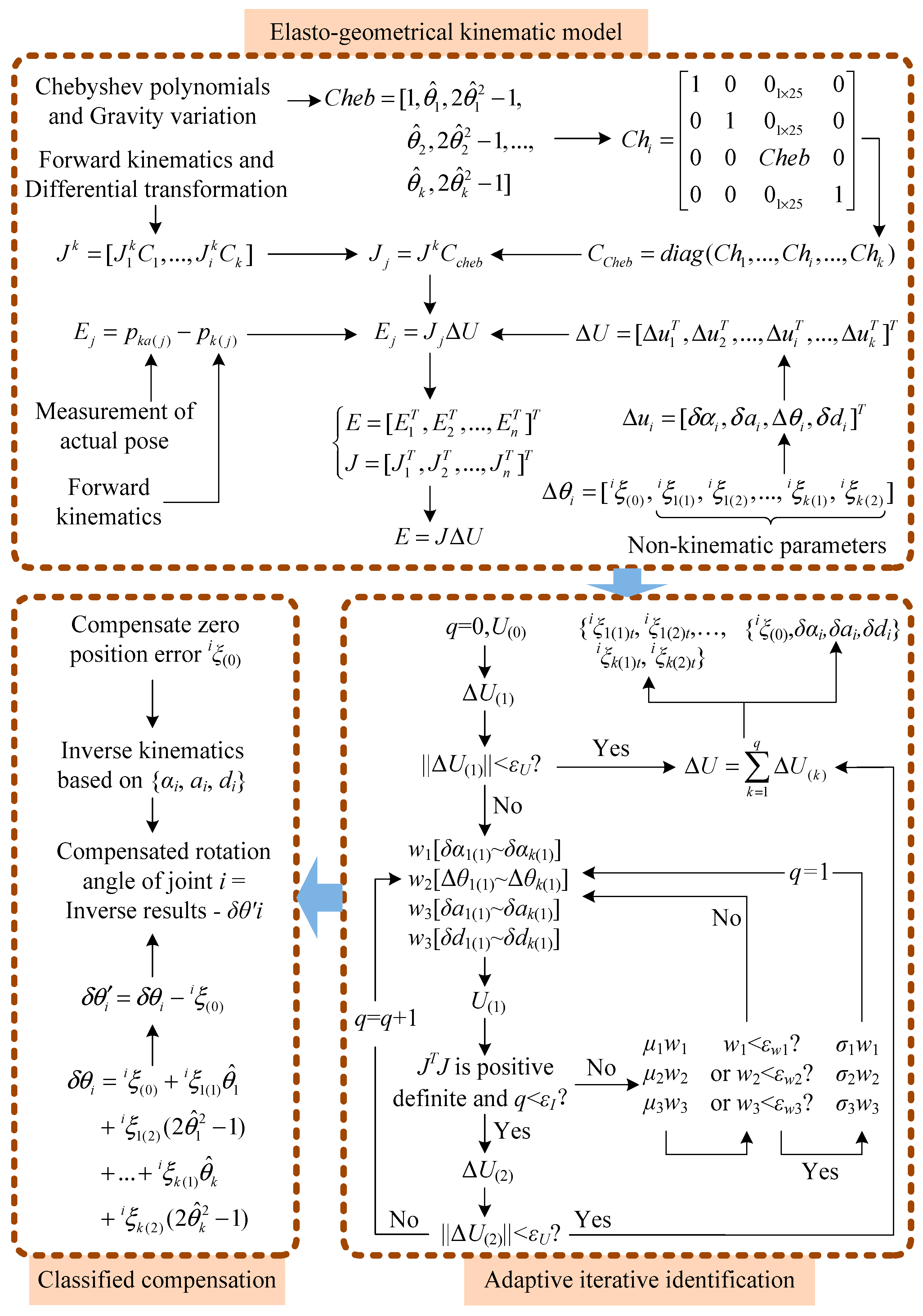
The calibration process is illustrated in Figure 2. The modeling procedure is detailed in Section 3, while the processes of the identification algorithm and the compensation algorithm are shown in the “adaptive iterative identification” and “classified compensation” modules in Figure 2, respectively.

Step 1: Let the MDH parameters of the robot arm at the j-th measurement configuration obtained from the q-th iteration be denoted as U_(q) = [α_1(q), a_1(q), θ_1(q), d_1(q), …, α_i(q), a_i(q), θ_i(q), d_i(q), …, α_k(q), a_k(q), θ_k(q), d_k(q)]^T. When q = 0, U₍₀₎ represents the nominal MDH parameters of the robot arm, where {θ₁₍₀₎, θ₂₍₀₎, …,θ_k(0)} are the joint angle commands at the j-th measurement configuration. Based on U₍₀₎, establish Equation (24). Define the result increment ΔU obtained from Equation (24) for the first time as the first identification result ΔU₍₁₎ = [δα₁₍₁₎, δa₁₍₁₎, Δθ₁₍₁₎, δd₁₍₁₎, …, δα_i(1), δa_i(1), Δθ_i(1), δd_i(1), …, δα_k(1), δa_k(1), Δθ_k(1), δd_k(1)]^T, where q = 1. If ||ΔU₍₁₎|| < ε_U, where ε_U is a predefined threshold, the iteration stops, and ΔU₍₁₎ is considered the final identification result. If ||ΔU₍₁₎|| ≥ ε_U, proceed to the next step.

Step 2: Multiply the set {δα₁₍₁₎, …, δα_k(1)} in ΔU₍₁₎ by the weight w₁ and then add them, respectively, to the set {α₁₍₀₎, …, α_k(0)} in U₍₀₎ to obtain {α₁₍₁₎, …, α_k(1)}. Multiply the set {Δθ₁₍₁₎, …, Δθ_k(1)} by the weight w₂ and substitute w₂{Δθ₁₍₁₎, …, Δθ_k(1)} and {θ₁₍₀₎, …, θ_k(0) } into Equations (4) and (5) to obtain {δθ₁₍₁₎, …, δθ_k(1)}, then add them, respectively, to {θ₁₍₀₎, …, θ_k(0)} to get {θ₁₍₁₎, …, θ_k(1)}. Multiply the sets {δa₁₍₁₎, …, δa_k(1)} and {δd₁₍₁₎, …, δd_k(1)} by the weight w₃ and then add them, respectively, to the sets {a₁₍₀₎, …, a_k(0)} and {d₁₍₀₎, …, d_k(0)} to obtain {d₁₍₁₎, …, d_k(1)}. The weights w₁, w₂, and w₃ need to be manually set, and usually 0 < {w₁, w₂, w₃} ≤ 1. Based on U₍₁₎ = [α₁₍₁₎, a₁₍₁₎, θ₁₍₁₎, d₁₍₁₎, …, α_k(1), a_k(1), θ_k(1), d_k(1)]^T, the calibration model of Equation (24) can be re-established.

Step 3: If the matrix J^TJ is positive definite and the number of iterations is less than ε_I, then ΔU₍₂₎ can be directly obtained from Equation (24) and let q = q + 1. Here, ε_I is a threshold set manually. If the matrix J^TJ is negative definite or semi-positive definite or the number of iterations reaches ε_I, then multiply w₁, w₂, and w₃ by the reduction coefficients to get μ₁w₁, μ₂w₂, and μ₃w₃, respectively (μ₁, μ₂, and μ₃ need to be set manually, and usually 0 < {μ₁, μ₂, μ₃} < 1), and re-execute Step 1 to establish Equation (24) with q unchanged.

Step 4: Repeat Steps 1 to 3 until w₁ < ε_w1, w₂ < ε_w2, or w₃ < ε_w3 still holds while ||ΔU_(q)|| ≥ ε_U, at which point the iteration stops. Multiply w₁, w₂, and w₃ by the reduction coefficients to get σ₁w₁, σ₂w₂, and σ₃w₃, respectively, then let q = 1 and execute Steps 1 to 3. Here, ε_w1, ε_w2, ε_w3, σ₁, σ₂, and σ₃ need to be set manually, and usually 0 < {σ₁, σ₂, σ₃} < 1. If ||ΔU_(q)|| < ε_U, then the iteration stops. Now, ΔU can be obtained by

$$\Delta U={\displaystyle \sum _{k=1}^q\Delta U_{(k)}}.$$

(25)

Step 5: In each load condition, the corresponding identification result ΔU can be obtained. If there are six sets of loads, then a total of six sets of ΔU will be obtained. Since ⁱξ₍₀₎, δα_i, δa_i, and δd_i are independent of joint elasticity, they do not change with the load. Therefore, the average values of ⁱξ₍₀₎, δα_i, δa_i, and δd_i from the six sets of ΔU are taken as the final identification results. However, {ⁱξ₁₍₁₎, ⁱξ₁₍₂₎, ⁱξ₂₍₁₎, ⁱξ₂₍₂₎, …, ⁱξ_k(1), ⁱξ_k(2)} represent joint elasticity and thus vary with the load. Therefore, their sample set is constructed as shown in

Table 1. Sample set of identification results of i-th non-kinematic parameters under multiple loads.

i-th Non-Kinematic Parameters	mF1	mF2	mF3	mF4	mF5	mF6
iξ1(1)	iξ1(1)(mF1)	iξ1(1)(mF2)	iξ1(1)(mF3)	iξ1(1)(mF4)	iξ1(1)(mF5)	iξ1(1)(mF6)
iξ1(2)	iξ1(2)(mF1)	iξ1(2)(mF2)	iξ1(2)(mF3)	iξ1(2)(mF4)	iξ1(2)(mF5)	iξ1(2)(mF6)
iξ2(1)	iξ2(1)(mF1)	iξ2(1)(mF2)	iξ2(1)(mF3)	iξ2(1)(mF4)	iξ2(1)(mF5)	iξ2(1)(mF6)
iξ2(2)	iξ2(2)(mF1)	iξ2(2)(mF2)	iξ2(2)(mF3)	iξ2(2)(mF4)	iξ2(2)(mF5)	iξ2(2)(mF6)
…	…	…	…	…	…	…
iξk(1)	iξk(1)(mF1)	iξk(1)(mF2)	iξk(1)(mF3)	iξk(1)(mF4)	iξk(1)(mF5)	iξk(1)(mF6)
iξk(2)	iξk(2)(mF1)	iξk(2)(mF2)	iξk(2)(mF3)	iξk(2)(mF4)	ξk(2)(mF5)	iξk(2)(mF6)

.

In Table 1, the subscripts “(m_F2)” and “(m_F3)” represent the identification results of the non-kinematic parameters {ⁱξ₁₍₁₎, ⁱξ₁₍₂₎, …, ⁱξ_k(1), ⁱξ_k(2)} under the loads m_F2 and m_F3, respectively. When a tool with a known weight m_t is installed at the end of the robot arm, the sample interval where m_t is located is first determined (here it is assumed that m_t in [m_F2, m_F3]), and in actual implementation, it is determined according to the actual situation). Then, based on Table 1 and the following formula, linear interpolation can be performed to obtain the identification results of the non-kinematic parameters corresponding to the external load {ⁱξ_1(1)t, ⁱξ_1(2)t, …, ⁱξ_k(1)t, ⁱξ_k(2)t}.

$$\left\{\begin{array}{l}{}^i\xi _{1(1)t}={}^i\xi _{1(1)(m_{F2})}+{\displaystyle \frac{m_t-m_{F2}}{m_{F3}-m_{F2}}}[{}^i\xi _{1(1)(m_{F3})}-{}^i\xi _{1(1)(m_{F2})}]\\ {}^i\xi _{1(2)t}={}^i\xi _{1(2)(m_{F2})}+{\displaystyle \frac{m_t-m_{F2}}{m_{F3}-m_{F2}}}[{}^i\xi _{1(2)(m_{F3})}-{}^i\xi _{1(2)(m_{F2})}]\\ \dots \\ {}^i\xi _{k(1)t}={}^i\xi _{k(1)(m_{F2})}+{\displaystyle \frac{m_t-m_{F2}}{m_{F3}-m_{F2}}}[{}^i\xi _{k(1)(m_{F3})}-{}^i\xi _{k(1)(m_{F2})}]\\ {}^i\xi _{k(2)t}={}^i\xi _{k(2)(m_{F2})}+{\displaystyle \frac{m_t-m_{F2}}{m_{F3}-m_{F2}}}[{}^i\xi _{k(2)(m_{F3})}-{}^i\xi _{k(2)(m_{F2})}]\end{array}\right.$$

(26)

Step 6: Based on the identification results obtained in Step 5, the compensation of ΔU is carried out in three sub-steps. First, for i = 1~k, take ⁱξ₍₀₎ from ΔU at any measurement configuration as the zero-position error of the i-th joint, and then compensate all ⁱξ₍₀₎ synchronously in the control system. Next, add {δα_i, δa_i, δd_i} from ΔU to {α_i, a_i, d_i} from U₍₀₎, respectively, to obtain the actual values {α_i, a_i, d_i} for the inverse kinematic solution (details are not repeated here). Finally, for i = 1~k, subtract δθ’_i from the joint i rotation angle command obtained from the inverse solution to obtain the final compensated rotation angle commands for all joints. Here, δθ’_i is

$$\delta {\theta }_i^{\prime }=\delta {\theta }_i-{}^i\xi _{(0)}.$$

(27)

The δθ_i in Equation (27) is obtained by first performing linear interpolation as described in Step 5 to get {ⁱξ_1(1)t, ⁱξ_1(2)t, …, ⁱξ_k(1)t, ⁱξ_k(2)t} and then substituting these values into Equation (4) to perform calculations at the corresponding joint rotation angle commands obtained from the inverse solution.

5. Simulation

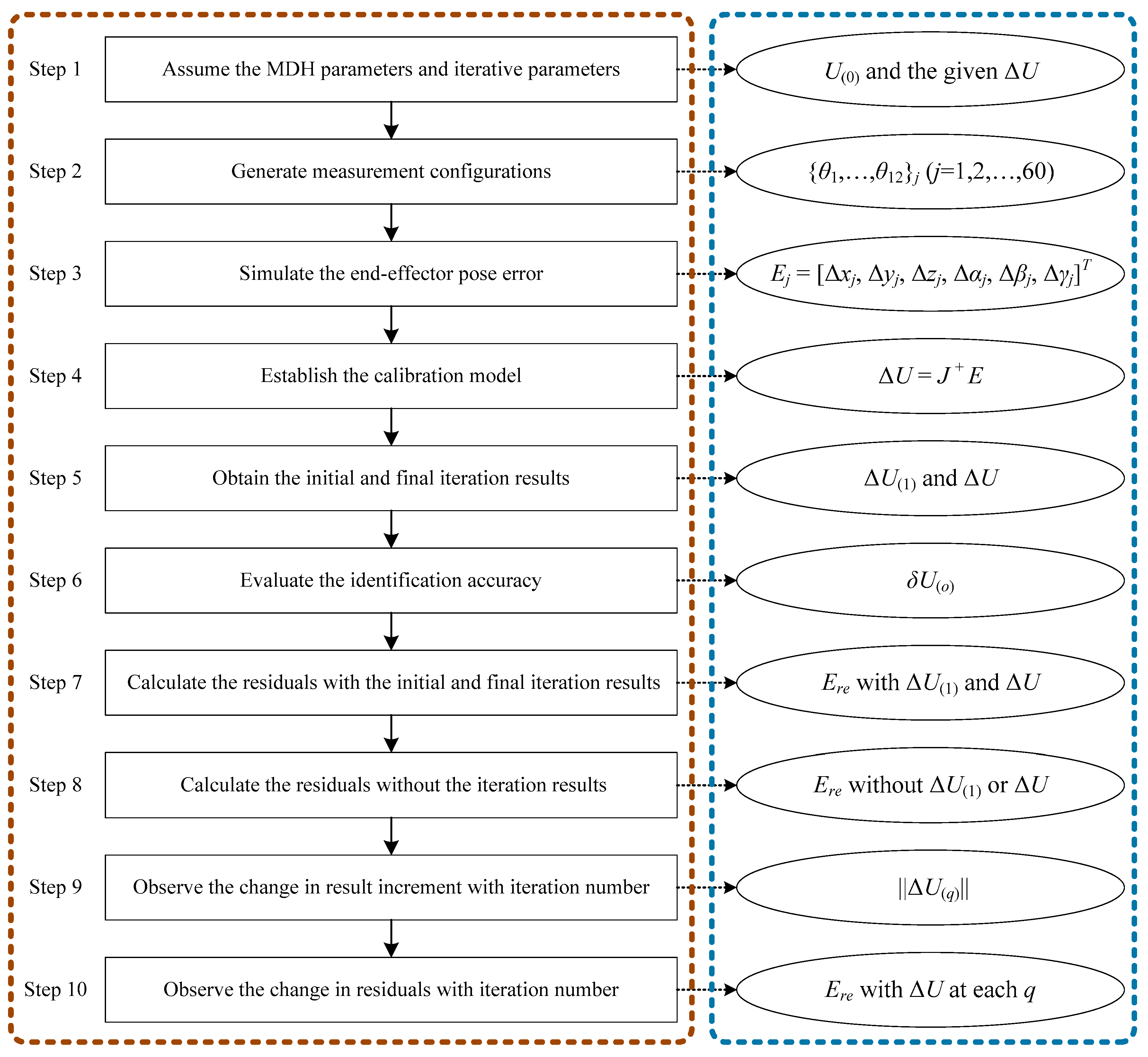
The simulation is performed on the MATLAB platform (R2023b, 2.10 GHz CPU). The procedure of the simulation is summarized in Figure 3.

Step 1: According to the joint numbers adopted by most hyper-redundant robot arms, here, let k = 12, and assume that the nominal values of the MDH parameters of the redundant robot arm are as shown in

Table 2. Assumed nominal kinematic parameters in simulation.

Joint	α (°)	a (mm)	θ (°)	d (mm)
1	−90	100	θ1	0
2	90	0	θ2	0
3	−90	100	θ3	0
4	90	0	θ4	0
…	…	…	…	…
11	−90	100	θ11	0
12	90	0	θ12	0

, where the values are similar to those of our self-developed prototype. The MDH parameter error values and non-kinematic parameter values are as shown in

Table 3. Assumed nominal non-kinematic parameters in simulation.

δαi (rad)	δai (mm)	iξ(0) (rad)	δdi (mm)	iξ1(1)~iξ12(2) (rad)
−0.01	−2	0.01	−2	0.002

, where ⁱξ₁₍₁₎~ⁱξ₁₂₍₂₎ are set based on the elasticity of the material used for the joint drive cables in our prototype. The structural parameters {δα_i, δa_i, ⁱξ₍₀₎, δd_i} are set according to the arm assembly error and zero position error, where the values are larger than those usually observed on industrial robots because the cable-driven robot arm is difficult to manufacture and assemble with very high precision. The error data obtained in previous studies [28,29,30] were also used as the basis for the assumed values. The iterative parameters are w₁ = 1; w₂ = w₃ = 0.5; σ₁ = σ₂ = σ₃ = 0.5; and μ₁ = μ₂ = μ₃ = 0.5, where the values are set according to our experience that the initial results of δα_i and ⁱξ₍₀₎ are relatively accurate, while those of δa_i, δd_i and ⁱξ₁₍₁₎~ⁱξ₁₂₍₂₎ have large identification errors in most cases. The thresholds are ε_U = 0.00001; ε_I = 200; ε_w1 = 0.01; and ε_w2 = ε_w3 = 0.005.

Step 2: Use the DETMAX algorithm [7,8,9] to select the measurement configurations {θ₁, …, θ₁₂}_j (j = 1, 2, …, 60).

Step 3: Simulate the end-effector pose error vector E. The elements of the pose error E_j = [Δx_j, Δy_j, Δz_j, Δα_j, Δβ_j, Δγ_j]^T required in Equation (21) are obtained as follows

$${({}^{0}T_{12})}^{-1}({}^{0}T_{12a})=\left[\begin{array}{cccc}0& -\Delta {\gamma }_j& \Delta {\beta }_j& \Delta x_j\\ \Delta {\gamma }_j& 0& -\Delta {\alpha }_j& \Delta y_j\\ -\Delta {\beta }_j& \Delta {\alpha }_j& 0& \Delta z_j\\ 0& 0& 0& 0\end{array}\right]$$

(28)

where ⁰T_12a is obtained with the following equation in the case of {θ₁, …, θ₁₂}

$${}^{0}T_{12a}={}^{0}T_{1a}{}^{1a}T_{2a}\dots {}^{(i-1)a}T_{ia}\dots {}^{12a}T_{12a}.$$

(29)

In Equation (29), ^(i−1)aT_ia represents the actual ⁽ⁱ⁻¹⁾T_i affected by Δu_i, which is obtained by replacing {α_i, a_i, θ_i, d_i} in Equation (2) with {α_i + δα_i, a_i + δa_i, θ_i + δθ_i, d_i + δd_i}. Here, δα_i, δa_i, and δd_i are given in Table 3, and δθ_i is obtained from Equation (4), {θ₁, …, θ₁₂}_j, and {ⁱξ₍₀₎, ⁱξ₁₍₁₎, ⁱξ_i(2), …, ⁱξ₁₂₍₁₎, ⁱξ₁₂₍₂₎} in Table 3. In Equation (28), ⁰T₁₂ is obtained from Equation (1) at i = 12 and the measured configuration {θ₁, …, θ₁₂}_j. By combining E_j at the 60 measured configurations according to Equation (23), the complete pose error vector E can be established.

Step 4: Substitute the obtained E into Equation (24) to establish the calibration model.

Step 5: Obtain ΔU₍₁₎ and ΔU according to Section 4.

Step 6: The identification accuracy of the o-th element in ΔU₍₁₎ and ΔU (where o represents the index of the error parameter in the ΔU vector) is denoted by δU_(o) and is calculated using the following equation

$$\delta U(o)=\left|{\displaystyle \frac{\Delta U_{ca}(o)-\Delta U(o)}{\Delta U(o)}}\right|\times 100(\%)$$

(30)

where ΔU_ca(o) is the identification result corresponding to the assumed value ΔU(o), and the identification accuracy δU(o) of ΔU₍₁₎ and ΔU is shown in Figure 4.

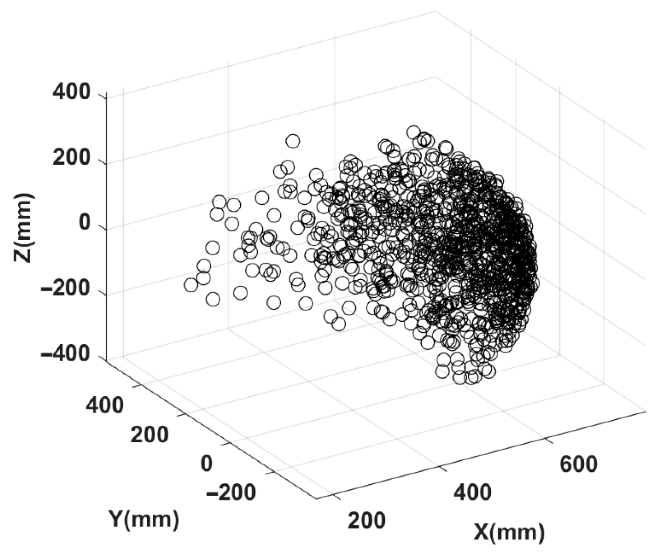
Step 7: Randomly generate 1000 measurement points within the workspace of the robot arm, as shown in Figure 5.

Then, compensate for the identification results of ΔU₍₁₎ and ΔU, respectively, and calculate the absolute positioning residual E_re of the 12th joint of the robot arm after the first calibration iteration of the new method and after the complete calibration iteration of the new method at the test-th measurement point (where test = 1, 2, …, 1000), using the following formula.

$$E_{re}=\sqrt{\Delta x_{test}^2+\Delta y_{test}^2+\Delta z_{test}^2}$$

(31)

The method for calculating the residuals after the first step of the new method’s iterative calibration and after the complete iterative calibration of the new method is similar to Equation (31). 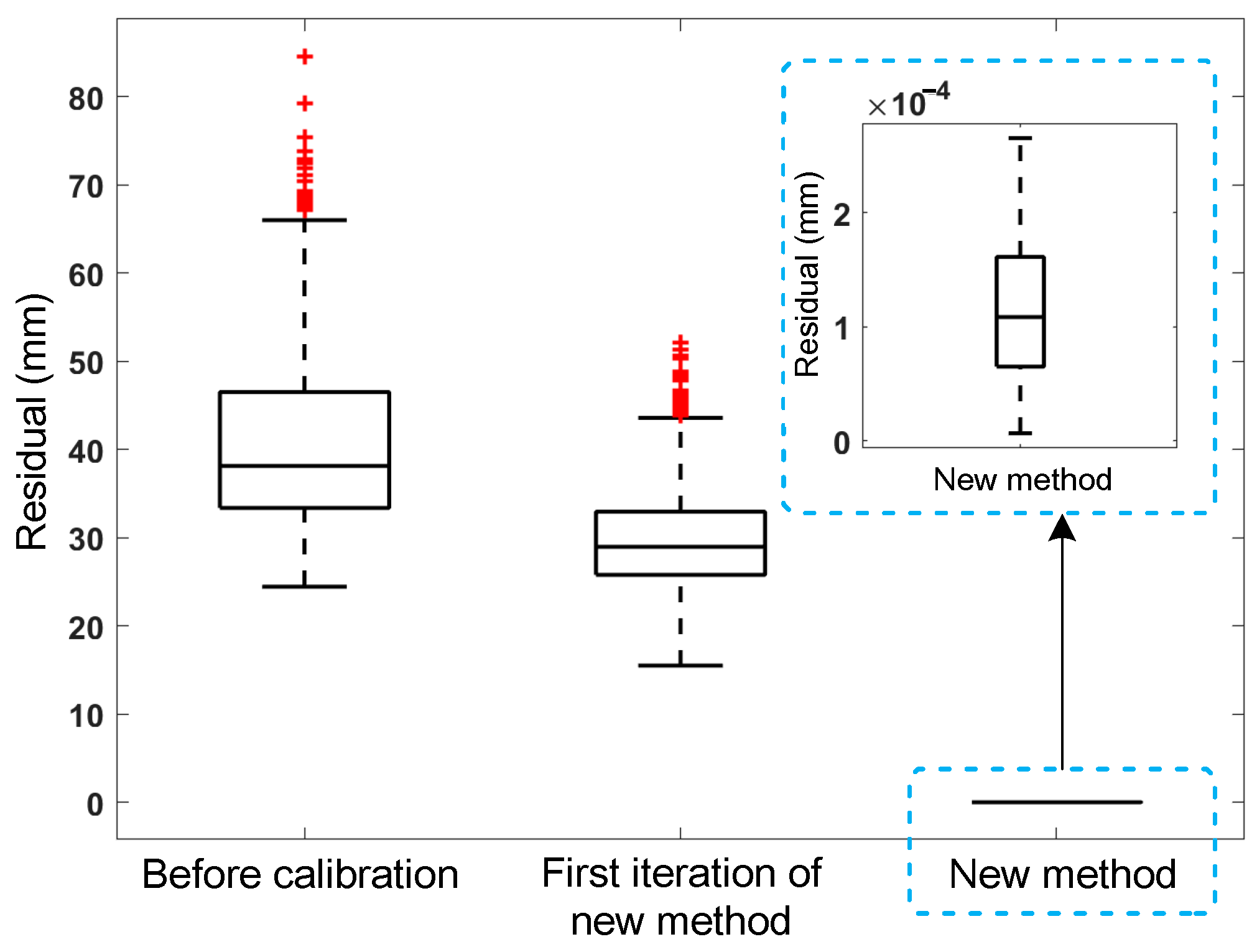The differences are that the measurement configurations j are all replaced by the measurement point test, and the values of δα_i, δa_i, δd_i, and {ⁱξ₍₀₎, ⁱξ₁₍₁₎, ⁱξ_i(2), …, ⁱξ₁₂₍₁₎, ⁱξ₁₂₍₂₎} are the corresponding identified values from ΔU₍₁₎ and ΔU. The statistical results of E_re for all measurement points are shown in Figure 6.

Step 8: Obtain the positioning error of the uncalibrated robot arm at measurement point test using a method similar to Equation (31), which serves as a control group for the two sets of residuals mentioned above. In Equation (31), Δx_test, Δy_test, and Δz_test are the corresponding components of E obtained in Step 3. The statistical results of the control group are also shown in Figure 6.

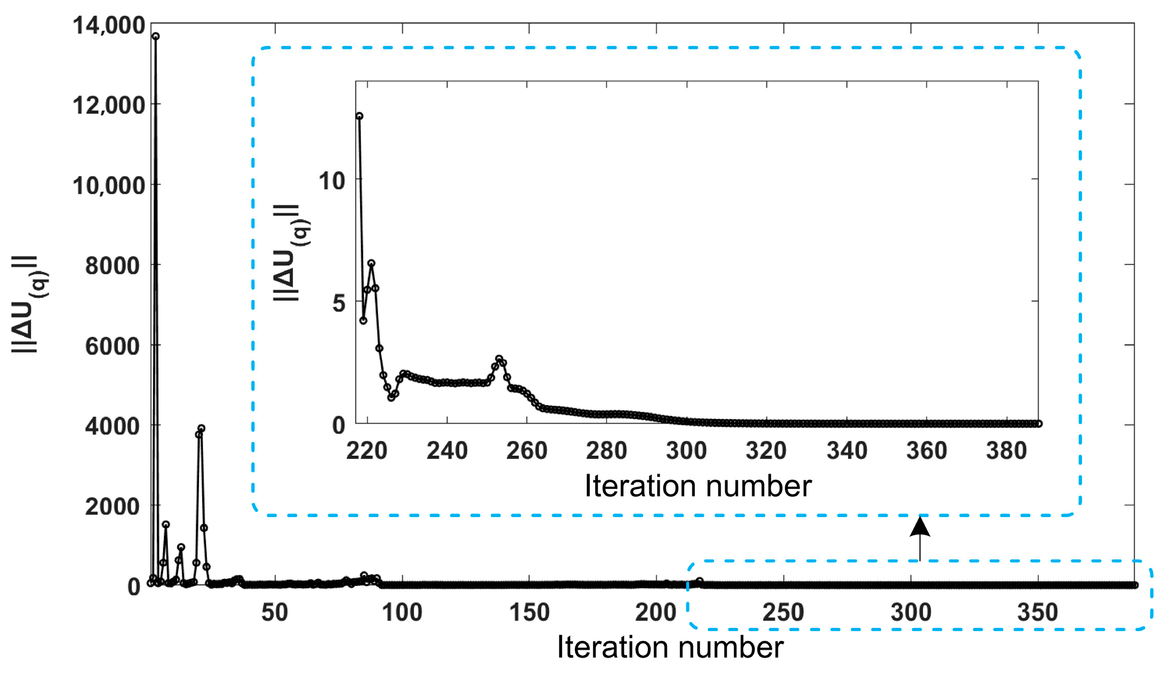
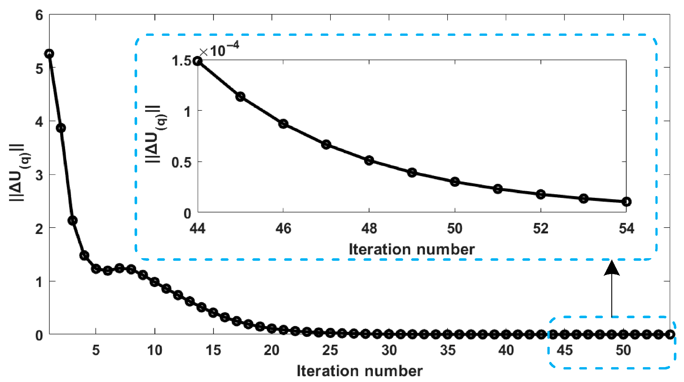
Step 9: Plot the values of ||ΔU_(q)|| obtained from each iteration of the new method, as shown in Figure 7.

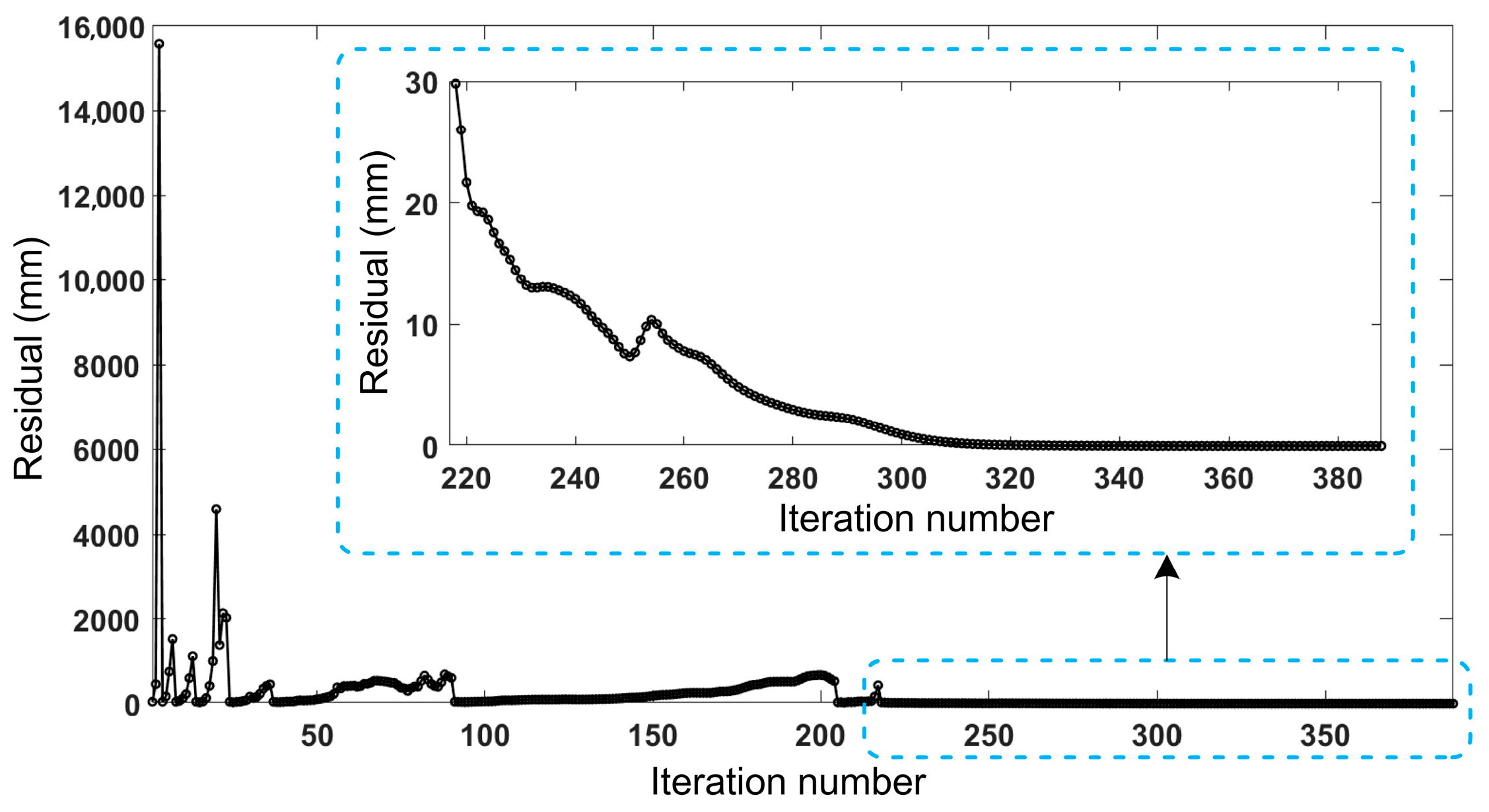
Step 10: After compensating for the identification results from each iteration of the new method, calculate the positioning residual of the robot arm at the 1000 measurement points using Equation (30). The results are shown in Figure 8.

Figure 4 indicates that the identification accuracies δU_(o) after the new method’s iterative convergence are all improved to be better than 0.025%, while some of those after the initial identification are extremely wrong (1 × 10³%~9 × 10³%). Figure 6 shows that the initial calibration and the iterative calibration using the new method can reduce the median residuals to 28.629 mm and 1.051 × 10⁻⁴ mm, respectively. Among them, the iterative calibration using the new method achieves the smallest residual, improving the calibration accuracy to about 99.975%. 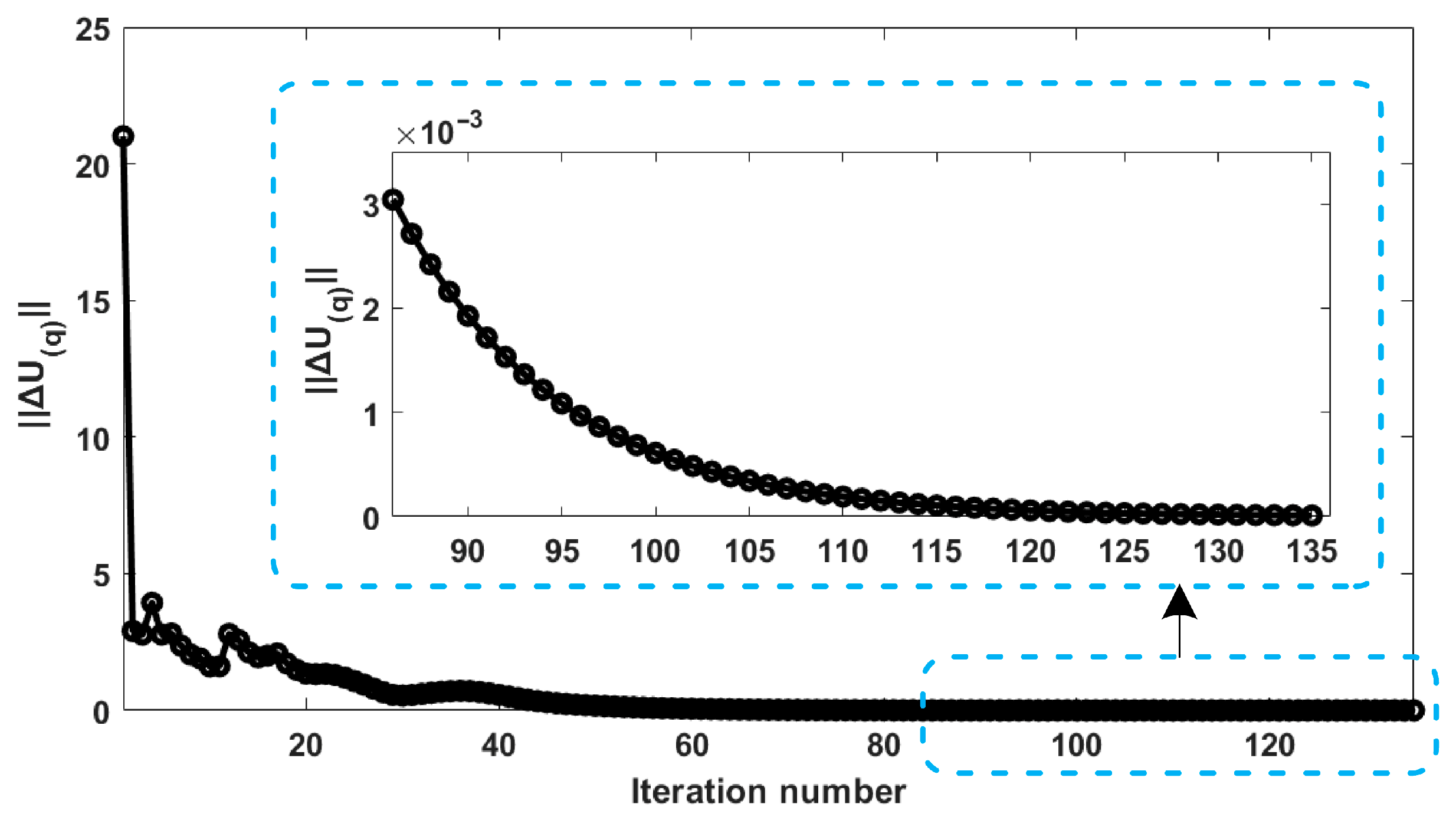Figure 7 demonstrates that ||ΔU_(q)|| gradually decreases with the increase in the number of iterations and eventually tends towards a stable and small value (smaller than 0.00001). Figure 8 shows that the positioning residuals gradually decrease with the increase in the number of iterations and finally stabilize. 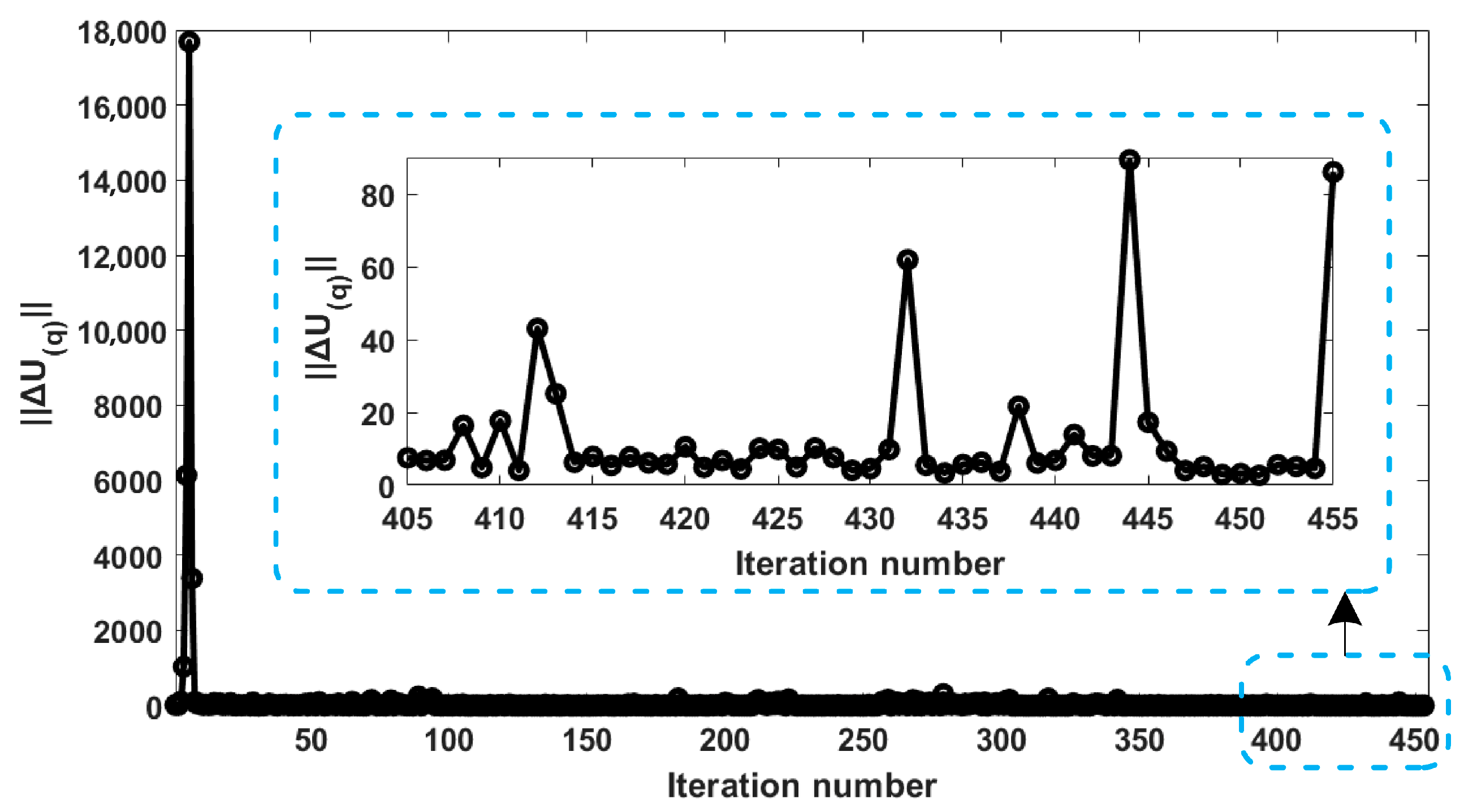The curves in Figure 7 and Figure 8 exhibit several inflection points where the residuals do not decrease but increase before convergence. This occurs when the iteration encounters a situation where J^TJ is not positive definite, leading to a tendency for the iteration to diverge. However, the adaptive weighting strategy of the identification algorithm enables ||ΔU_(q)|| and the positioning residuals to quickly resume their downward trend and ultimately converge. The overall results show that the new method achieves a generalized representation of non-kinematic errors and enhances the completeness of the calibration model, more accurately representing the coupled characteristics of the robot arm’s rigidity and flexibility. Moreover, the new method overcomes the problem of the increased linearization errors caused by the dramatic increase in the dimensions of non-kinematic parameters through an iterative identification algorithm, ensuring the accuracy of parameter identification.

6. Experiment

6.1. Experiment Setup

A redundant robot arm with eight degrees of freedom (DOFs) is adopted here. Although this reduces the number of elastic joints compared with the 12 joints assumed in the simulation, this elastic robotic arm with 8 joints also has a high error model dimension (6n × 224), where the effectiveness of the new identification algorithm on the high-dimensional error model of highly elastic robotic arms can also be demonstrated. The experiment is conducted at room temperature of 25 °C (with air-conditioning on). The nominal kinematic parameters are listed in

Table 4. Nominal kinematic parameters in experiment.

Joint	α (°)	a (mm)	θ (°)	d (mm)
1	0	117.160	θ1	0
2	90	0	θ2	0
3	−90	110	θ3	0
4	90	0	θ4	0
…	…	…	…	…
7	−90	110	θ7	0
8	90	0	θ8	0

. The main specifications of the vision system are listed in

Table 5. The main specifications of the vision system.

Instruments	Parameters	Values
HN-P-1624-25M-C1.2/1 lens	Focal length	15.96 mm
	FOV	48.83° (H) × 42.86° (V)
ME2P-2622-15U3M/C camera	Resolution	5120 (H) × 5120 (V) pixels
	Pixel size	2.5 μm × 2.5 μm

.

As shown in Figure 9, a marker (named marker-1) with a size of 50 mm × 50 mm is set close to the end of robot. The camera is located properly to ensure that the workspace of the robot can be entirely contained by the FOV (field of view).

Here, a laser tacker (API Radian PLUS with distance resolution of 0.5 μm and maximum permissible error of 15 μm + 5 μm/m) is also adopted to increase the accuracy of preparation. As shown in Figure 10a, due to the high precision in the manufacturing of the marker, touching the edge and surface of the marker with the laser tracker’s spherically mounted reflector (SMR) can fit the outer contour dimensions of marker-1 in the laser tracker coordinate system F_L. This allows for the establishment of F_m1, as shown in the figure. By moving joint 8 of the robot arm to several rotation angles and performing the above operations at each angle, ^LT_m1 at each angle can be obtained. Fitting the origins of this series of ^LT_m1 into an arc yields the central axis of the arc, whose unit vector is the axis Z₈ of joint 8. The same method is used to establish the axis Z₇ of joint 7, and then F₈ at each angle is established, as shown in the figure. Combining the corresponding F_m1 with it results in a constant ⁸T_m1.

In addition, compared with traditional robot arms, flexible redundant robot arms have much higher flexibility and larger absolute positioning errors. Therefore, traditional hand–eye calibration methods cannot obtain an accurate transformation matrix ^cT₀. To address this, as shown in Figure 10b, we adopted a dual-target pose transfer method to achieve hand–eye calibration for flexible redundant robot arms. Specifically, a target (marker-2) with the same size of marker-1 was set up next to the robot arm base, and it was precisely installed so that the transformation ^m2T₀ from its coordinate system F_m2 to the base frame F₀ is accurate. Similarly to ^LT_m1, the SMR of the laser tracker was used to obtain ^LT_m2. The robot arm was adjusted to a suitable posture so that the camera could accurately measure the pose of marker-1, i.e., accurately obtain ^cT_m1. A method similar to that for ^LT_m2 was used to obtain ^LT_m1 at this time. Thus, ^cT₀ = (^cT_m1)(^m1T_L)(^LT_m2)(^m2T₀)⁻¹ can be obtained.

It should be noted that joint elasticity can cause obvious vibrations in the robotic arm. Therefore, after the robotic arm reaches each specified configuration, it is necessary to wait for about 5 s, that is, until the vibrations of the robotic arm stop, before carrying out the pose measurement. In addition, improper force control when the SMR touches marker-1 can also cause marker-1 to deviate from its correct position. Therefore, it is necessary to synchronously observe in real time whether there is a significant change in the pose of marker-1 on the camera at this time. The change in the position of marker-1 should be less than the camera’s repeatability measurement accuracy, which is 0.06 mm along both the X_c and Y_c axes and 0.13 mm along the Z_c axis, considering the camera’s characteristics in Table 5 and the measurement distance of 400 mm.

It should be explained that the measurement method described above, which employs a camera as the measuring instrument, allows for the use of lightweight markers as sensors. This method is suitable for the lightweight cable-driven robot arm used in this paper. When the measurement object is an elastic robot arm with a higher load-bearing capacity to move the SMRs, it is possible to consider using the commonly used laser tracker as the measuring device. In this way, not only can the series of preparations to improve the measurement accuracy of the vision system be avoided, but also a higher measurement accuracy can be achieved.

6.2. Pose Measurement and Parameter Identification

A total of 60 measurement configurations are selected according to the DETMAX algorithm and marker visibility, and some of them are presented in Figure 11. It is seen that the marker can be clearly seen by the camera at each pose. To minimize the influence of measurement noise, 50 pictures are taken for each marker at each measurement configuration. Marker-1 is considered one of the external loads described in Table 1. After collecting sufficient end-effector pose errors of the robot arm according to the above steps, the identification model can be established based on Section 2.

Then the proposed identification algorithm (the method is denoted by M1) can be executed. It should be noted that the iterative parameter values of the identification algorithm in the experiment are slightly different from those in the simulation. They are set as w₁ = w₂ = w₃ = 1; σ₁ = σ₂ = σ₃ = 0.5; μ₁ = 0.8; and μ₂ = μ₃ = 0.5. It has to be explained that the joint number in the experiment is lower than that in the simulation, so the dimension of the error model is reduced. Accordingly, the initial identification errors of δa_i and δd_i will also be reduced; thus, w₂ and w₃ increase from 0.5 to 1. In addition, the value of μ₁ increases from 0.5 to 0.8 because the identification errors in each iteration of δα_i and ⁱξ₍₀₎ will also be reduced with the dimension of the error model. The thresholds ε_U, ε_I, ε_w1, ε_w2, and ε_w3 are the same as those in the simulation. Also, the identification algorithms proposed in Ref. [26] (the method is denoted by M2) and Ref. [27] (the method is denoted by M3) are adopted to the new calibration model for a comparison with the new adaptive iterative identification algorithm M1.

6.3. Experimental Results and Discussion

The changes in ||ΔU_(q)|| with iteration number in the cases of the three identification algorithms are represented in Figure 12, Figure 13 and Figure 14, respectively. For M1, as shown in Figure 12, the identification stops at the 135th iteration, which takes 29.077 s. Similarly to the results in Figure 7, for ||ΔU_(q)|| in Figure 12, as the number of iterations increases, the value gradually decreases and eventually stabilizes at a very small value (smaller than 0.00001). Before convergence, the curve exhibits several inflection points where it does not decrease but instead increases, indicating a tendency towards divergence at these points. However, the adaptive weighting strategy of the identification algorithm enables ||ΔU_(q)|| and the positioning residual to quickly resume their downward trend and ultimately converge. For M2, as shown in Figure 13, the iteration does not converge and keeps oscillating within a very large range of ||ΔU_(q)||, which indicates that algorithm M2 fails when facing the high-dimensional calibration model. For M3, as shown in Figure 14, the identification stops at the 135th iteration. Although M3 converges to the same high precision (smaller than 0.00001) as M1 and has the fewest iterations, the total time consumed by M3 is 124.905 s, which is much longer than that consumed by M1. The convergence in Figure 12 demonstrates that the modeling method and the corresponding adaptive identification algorithm proposed in this paper also have good applicability and convergence in practical use.

Also, a comparison similar to that in Steps 7 and 8 in Section 5 is also performed here; that is, the absolute positioning residual of the robot arm before calibration, after one iteration of the algorithm, and after multiple iterations of the algorithm have converged is compared to evaluate the advantage of the new calibration method in the real world. It should be noted that the error compensation still follows the “classified compensation” module process shown in Figure 3. However, since the experiment uses a cable-driven flexible robot arm, after compensating for the joint angles of the arm, it is also necessary to additionally convert them into the extension and contraction amounts of the drive cables and instruct the drive motors to make corresponding output angle adjustments (the details of which are omitted here as they are not the focus of this paper). Here, we randomly generated another 100 measurable configurations for verifying the calibration accuracy and still used an industrial camera to measure the end-effector residual of the robot arm, the results of which are shown in Figure 15.

Similar conclusions to those in Figure 6 can be drawn from Figure 15, which shows that the initial calibration and the iterative calibration of the new method can reduce the median residuals to 31.929 mm and 2.988 mm, respectively. Among them, the iterative calibration of the new method achieves the smallest residual. It should be noted that by comparing the residual values shown in Figure 6 and Figure 13, it can be seen that even after optimization by the new calibration method, the absolute residual of the redundant robot arm in the experiment was reduced, but it is still much higher than that in the simulation. This indicates that there are many sources of error in the elastic redundant robot arm in practical applications. These errors are coupled with each other and mapped to the end-effector pose error, making it difficult for their identification and compensation to reach the accuracy level of those of traditional industrial robot arms. Specifically, as the pose of the arm changes, the pressure between the cable and the cable hole will change. This change will lead to a change in the friction force between the cable and the cable hole, and this friction force has a coupled effect on the end-effector pose with the joint elasticity. In addition, since the stiffness of the slender joint hinges of the self-developed cable-driven robotic arm is much lower than that of the robust joints of industrial robotic arms, the flexibility error of a certain joint’s hinge structure will be coupled with the flexibility error of the joint that is perpendicular to it. Even so, the new method proposed in this paper can already control the absolute positioning residual of the elastic redundant robot arm to a relatively low value, enabling it to be used in applications such as detection and grasping that have general working accuracy requirements.

It is worth mentioning that although the new modeling method and identification algorithm are proposed based on a highly elastic cable-driven robot arm, the method can be extended to other types of manipulators simply by adjusting the parameter values in the modeling and identification stages. For instance, in the case of the 6-DOF industrial robot, the order of Chebyshev polynomials in Equation (4) can be reduced to one or zero, since the joints are more rigid than those of the cable-driven ones. Also, all of the iterative parameters (except the thresholds) can be increased to be close to 1. The same strategy can be applied to the collaborative robot where the joints are more elastic than those of rigid industrial robots but more rigid than those of cable-driven ones.

The iterative identification algorithm proposed in this paper is specifically designed for the error parameters of the new model. Therefore, the adaptive adjustment strategy of this algorithm in the iteration has certain limitations; that is, it aims to gradually eliminate the identification errors caused by various kinematic and non-kinematic error parameters in each round of iteration. In fact, some researchers have proposed more widely applicable parameter identification algorithms. For instances, Sanin-Villa et al. tackled parameter estimation for thermoelectric generators using the Salps Search Algorithm, achieving impressively high consistency and accuracy [31]; they also compared metaheuristic algorithms for the inverted pendulum system, with the SSA delivering highly accurate and reliable results [32]. These algorithms have strong generalization ability and provide valuable references for our future optimization of the identification algorithm in this paper.

7. Conclusions

The calibration method for high-elastic redundant robot arms proposed in this paper, which couples rigidity and flexibility, demonstrated good model accuracy and identification accuracy in both simulations and experiments. In the experiments, we found that the base-fixed camera (which is also the installation form adopted by the vast majority of measuring devices) could hardly cover all the optimal measurement configurations of the redundant robot arm. Therefore, in the actual measurements, we used some measurable suboptimal configurations to replace the optimal measurement configurations that could not be measured. However, the pose data collected in this way could not fully cover the rotation space of each joint, and the calibration model established based on this was prone to ill-conditioning. In contrast, if the complete optimal measurement configurations could be captured, the coverage of the pose data would be more comprehensive, and the calibration model established would achieve the optimal condition level, with more accurate identified parameter values.

To address this issue, in the future, we plan to conduct research on our self-developed mobile-base measuring arm. We aim to make targeted pose adjustments for each optimal measurement configuration of the redundant robot arm before performing the measurements, thereby improving the flexibility and accuracy of the measurements.