Abstract
Sustainable irrigation in water-limited regions requires timely, field-scale estimates of soil water content (SWC). Yet, field-scale SWC studies leveraging near-daily satellite imagery of regenerative systems—particularly cotton under Mediterranean conditions—are lacking, and explainable integrations of Planet SuperDove with agrometeorological inputs remain underexplored. In this study, we evaluated a machine learning framework that integrates near-daily multispectral features from Planet SuperDove with agrometeorological variables to estimate the daily SWC of regenerative cotton under Mediterranean conditions across two seasons (2023–2024). Six regression models were compared; extreme gradient boosting achieved the highest accuracy (R2 = 0.73 ± 0.08; RMSE = 4.60 mm ± 0.81; nRMSE = 0.035 ± 0.01), with limited bias and stable performance across the years and moisture conditions. The model interpretability via SHAP indicated that agrometeorological drivers contributed over half of the predictive power, while the NDVI and NIR provided the most informative satellite inputs, followed by the NDRE and PSRI. The results show that combining high-frequency satellite data with meteorological inputs can deliver accurate and interpretable SWC estimates at the homogeneous plot level, supporting irrigation optimization of regenerative systems. This approach is practical, transferable, and suited for operational decision-making where frequent, high-resolution observations are available.
1. Introduction
The availability of fresh water for agriculture is becoming one of the most limiting factors for global food security. Population growth and climate change—with rising temperatures and erratic rainfall—are exacerbating the pressures on water resources. Recent projections indicate that, without intervention, two-thirds of the world’s population could suffer the consequences of water scarcity [1]. In this scenario, improving water use efficiency in agricultural practices will be a priority for sustainable development. Indeed, conservative water management strategies—e.g., techniques such as micro-irrigation—are needed to reduce wastage and increase the water productivity of crops [1,2]. In addition, there is a growing focus on innovative agricultural approaches that aim to improve the health and resilience of agroecosystems, including conservative and regenerative agriculture [3], with the aim of combining productivity and the conservation of natural resources (soil, water, and biodiversity). For instance, regenerative agriculture practices—such as minimum tillage, cover crops, diversified crop rotations, and agroforestry [3]—aim to improve soil health by increasing the organic matter content and porosity. Regenerated soil shows an increased water infiltration and retention capacity, which results in longer water availability for plants after rainfall or irrigation [4]. However, in regenerative systems, the saving water technique remains an indispensable requirement in many agro-climatic contexts, especially for crops in arid or semi-arid areas. In Mediterranean climate regions, characterized by hot and dry summers, optimization of irrigation is needed to ensure productivity while reducing water consumption [5,6]. The Mediterranean area is already considered a water scarcity hotspot, and the irrigation demand is expected to increase further due to climate warming [7,8].
Technological innovation is providing new tools to support water saving in agriculture. Recent years have seen an increasing use of satellite remote sensing and machine learning models in precision agriculture, especially for monitoring the water status of crops and soil [9,10]. Satellite imagery—e.g., from high-resolution multispectral platforms such as Sentinel-2 or CubeSat (Planet) satellites—allows for frequent observation of trends in vegetative vigour, water stress, and other biophysical parameters of crops [11,12,13]. By integrating these data with advanced machine learning algorithms, it is possible to extract information to support agronomic decisions [14]. Machine learning enables the identification of complex, non-linear patterns, providing forecasts or estimates of variables of interest with a high level of automation and accuracy. For example, it has been shown that combining satellite data with machine learning models allows for monitoring the water stress of a crop and identifying when to apply irrigation, therefore mitigating the impact of soil water stress on the crop’s quality and yield [15,16]. In addition to reducing the need for manual field surveys and technical checks, this data-driven approach provides frequent and non-invasive monitoring of crop status, facilitating the transition to smarter, more targeted irrigation practices [17,18]. However, the applicability of such frameworks in commercial contexts is highly dependent on the temporal frequency of image acquisition, spectral resolution, and, clearly, the associated costs [19].
In the context of water management, a key variable to be monitored is the SWC, i.e., the amount of water in the soil profile that is accessible to the roots [20]. The SWC directly influences the water status of plants and crops’ water requirements; therefore, knowing its trend over time is important to optimize irrigation schedules and prevent both water stress and water consumption [21]. Direct measurements of SWC can be performed using in situ sensors. On the other hand, satellite observations specifically dedicated to soil moisture (such as SMAP or SMOS missions) provide global coverage, but with low spatial resolutions for field applications [22,23]. This means that such satellite data, while useful at regional or global scales, are less suitable for guiding irrigation decisions at the individual plot level, especially when the objective is to estimate the SWC of the root profile of crops. In this context, machine learning models can be a complementary solution to estimate the SWC. ML, through training on observed data, can capture the non-linear relationships between environmental variables (e.g., rainfall, evaporation, and vegetation cover) and the SWC. These data-driven models do not rely on predetermined physical assumptions, but “learn” from the data, and are thus able to take into account heterogeneous information (meteorological data, remote sensing indices, and sensor measurements) in a single estimation framework [24]. Different works have shown that the integration of multi-source data through ML algorithms significantly improves the soil moisture predicting power [25,26]. The application of such methods to water-intensive crops, such as cotton, is of particular importance. Cotton (Gossypium hirsutum, L., 1763) is one of the most widespread industrial crops in the world and represents the main source of natural textile fibre. Traditionally, cotton production has high water requirements [27]. This places cotton among the crops with the highest contribution to “unsustainable” water consumption on a global scale [28]. These values reflect both the large spread of irrigated areas dedicated to this plant and the high water requirements during the crop cycle, especially in the arid regions where cotton is cultivated. In intensive conventional systems, high water use is often associated with agronomic practices with high inputs of fertilizers and pesticides, with additional environmental impacts [29]. Cotton managed via regenerative practices can represent a regional opportunity for a more sustainable agricultural economy, as it aims to increase soil’s water infiltration and retention, reduce direct evaporation and the irrigation demand, and stabilize productivity during the hot, dry summers typical of the Apulian Mediterranean. Regenerative practices (e.g., vetch cover crops and minimum tillage) may alter soil cover, evaporation, and surface hydraulic properties throughout a season, creating both a challenge (rapid and non-linear SWC dynamics) and an opportunity for explainable models that integrate near-daily observations and agrometeorological variables at a homogeneous plot scale. Thus, it becomes important to develop reliable methods for estimating the SWC in cotton cultivation. The ability to predict the SWC using data-driven models could improve crop water productivity, avoiding both water excess and deficits. This is of particular importance in semi-arid environments, such as southern Italy, where irrigation water is a limited resource and can compromise agricultural activities and economic returns.
To the best of the knowledge of the authors, to date, no work has specifically addressed regenerative cotton systems under Mediterranean conditions, nor has any work exploited the integration of near-daily Planet SuperDove imagery with agrometeorological variables within an explainable framework. This combination can provide both innovative data use and unique agronomic relevance, potentially aiding in bridging the gap between sustainable farming practices and precision irrigation strategies. The objective of the present study was to develop an ML framework for estimating the SWC of a cotton crop managed using regenerative agriculture techniques in southern Italy. For this purpose, different ML algorithms were tested and compared, using agrometeorological information (reference evapotranspiration, rainfall) and high-frequency satellite data.
2. Materials and Methods
2.1. Site Description
The research was conducted at the experimental farm of the Council for Agricultural Research and Economics in Rutigliano, southern Italy (40°59′ N; 17°01′ E; 166 m a.s.l.). The farm holds an official Regenagri certification (www.regenagri.org) for the adoption of regenerative farming practices. The climate of the area is classified as CSa according to the Köppen and Geiger system, characterized by dry and hot summers and mild winters. The average annual rainfall is about 535 mm, with the majority occurring in the autumn and winter months, while precipitation is limited during the spring and summer, thus making it difficult to cultivate most crop species under non-irrigated conditions [30]. The soil at the farm is classified as clay loam according to the USDA system, consisting of 55% clay, 33% silt, and 15% sand. The stoniness is about 10%. The field capacity and wilting point are 36% and 22% of the volume water content, respectively. At a 0.50 m depth is a parent rock that reduces the capacity of the root systems to expand beyond this layer. The soil characteristics are homogeneous throughout the experimental farm.
2.2. Crop Management and Agrometeorological Information
Cotton, cv. ‘ST402’ (Pioneer, Athens, Greece), was cultivated during the 2023 and 2024 seasons in two different plots, A (0.70 ha) and B (1.80 ha), respectively (Figure 1). Plot A was left fallow before cotton cultivation, while in 2024 (plot B), a vetch cover crop (Vicia spp.) was incorporated as green manure prior to seedbed preparation in April. Cotton was sown at a seeding rate of 15 kg ha−1 on 30th May in the first year, and on 19th June in the second year (15 plants m−2 for both plots). The other cultivation practices were the same for both plots. Weed management was carried out under a minimum tillage approach, involving occasional shallow tilling of the soil, mainly during the early growth stages.
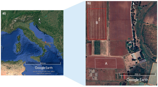
Figure 1.
Location of the experimental farm in southeastern Italy (a); experimental plots (b) where cotton was grown in 2023 (A) and 2024 (B).
Irrigation was supplied via surface drip lines with 4 L h−1 emitters at 30 cm spacing. The daily crop water use was computed with the FAO-56 approach: the reference evapotranspiration (ETo) from the FAO Penman–Monteith equation; the crop evapotranspiration, ETc = Kc × Eto, using tabulated Kc values (Kcini = 0.15; Kcmid = 1.10; Kcend = 0.50); and a management allowable depletion, p = 0.50, with stage-specific adjustments (FAO-56 recommendations) [31]. The net irrigation requirement was calculated as IN = ETc − effective rainfall, and the irrigation scheduling targeted 100% of IN. During peak demand (July–August), irrigations were typically executed at short intervals to track the rising ETc. The distribution of irrigation events for each year is reported in Figure 2. All the meteorological inputs were recorded by the on-farm agrometeorological station installed within the experimental area.
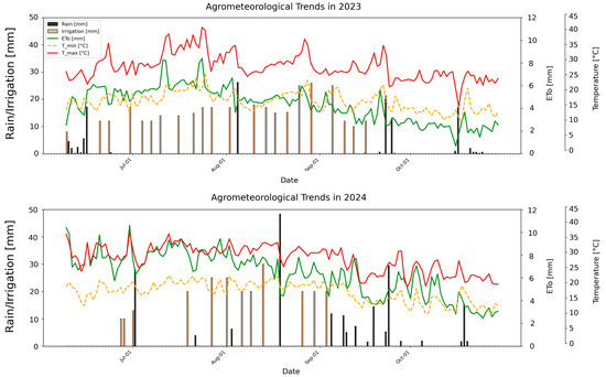
Figure 2.
Trend of minimum and maximum temperature (T_min and T_max), reference evapotranspiration (ETo), rainfall, and irrigation water applied during the two cotton growing seasons.
The soil moisture was continuously monitored in each experimental plot during both growing seasons using Teros 10 sensors (Meter Group, Pullman, WA, USA). The sensors were installed in paired vertical positions at two depths (0.20 m and 0.40 m) at each sampling location. Specifically, in plot A, two locations were randomly selected; instead, for plot B, due to its larger surface area, four random locations were chosen. The soil characteristics across the entire experimental area were homogeneous, and the crops did not show any evident growth variability or spatial heterogeneity that might indicate low representativeness of sensor measurements. The soil moisture data were recorded at 30 min intervals and subsequently aggregated to obtain the daily averages per plot and depth. Sensor readings of dielectric permittivity were converted to volumetric soil water content (%) using the equation provided by the manufacturer; therefore, the soil water content SWC (mm) for the entire soil profile (0.40 m) was determined as the sum of the water stored in each monitored layer, by multiplying the volumetric water content by the thickness of the corresponding soil layer (i.e., SWC = VWC × soil depth) [21].
2.3. Satellite Data and Vegetation Indices
Multispectral satellite images of the SuperDove constellation (Planet Labs PBC, San Francisco, CA, USA) were downloaded from the Planet platform (planet.com/explorer). SuperDove satellites acquire near-daily images with a spatial resolution of 3 m, measuring the reflectance in eight spectral bands, from the visible to the red edge and near-infrared (NIR) regions. For each cropping season, only cloud-free images were selected, resulting in a total of 132 images across the two growing seasons (Planet Imagery ©, 2023 and 2024). For each selected image, the following vegetation indices (VIs) were computed: the Normalized Difference Red-Edge Index (NDRE), Normalized Difference Vegetation Index (NDVI), Plant Senescence Reflectance Index (PSRI), and Green NDVI (GNDVI) (Table 1). These VIs were selected as the benchmarks for their established physiological and agronomic relevance in remote sensing applications for cotton and other field crops. The NDRE was chosen for its increased sensitivity to changes in canopy chlorophyll and water status under dense vegetation, making it valuable in the mid-to-late season when the NDVI may saturate [32]. The NDVI and GNDVI are considered useful indices because of their widespread use and ability to detect crop vigour, green biomass, and general plant health across a range of cropping systems; the PSRI, on the other hand, specifically targets the detection of leaf senescence and stress, providing information about the onset of physiological decline and its relationship with soil water status [33,34,35]. For each image from both plots, the median value was calculated for the reflectance of each individual SuperDove band (SDB) and for each derived vegetation index.

Table 1.
Vegetation indices (VIs) used in this study with their formula and reference.
2.4. Machine Learning
The prediction of SWC was conducted using a supervised machine learning regression framework implemented in Python (version 3.12.7, 64-bit; Spyder IDE version 6.0.1). The daily data for the plots from the two growing seasons, including the ETo (5-day moving average), cumulative rainfall, and satellite-derived features (the eight SDBs and the four calculated VIs), were merged and temporally aligned into a single dataset (n = 132). The SWC was used as the target variable, while all the other variables were used as predictors. Before modelling, the predictors were standardized (zero mean and unit variance) within the machine learning pipeline.
Five supervised regression models, random forest (RF), extreme gradient boosting (XGBoost), elastic net (EN), support vector regression (SVR), k-nearest neighbours (KNN), and linear regression (LR), were evaluated and compared. All the models were implemented using the scikit-learn library (v. 1.5.1) [36], except for XGBoost, which was implemented using the dedicated XGBoost Python package (v. 2.1.3) [37]. RF is an ensemble method based on decision trees, in which a large number of trees are built using random subsets of the training data and features; the final prediction is obtained by averaging the outputs of all the individual trees, a process that improves the stability and reduces overfitting. XGBoost is a gradient-boosting technique based on decision trees, optimized for computational efficiency and accuracy through advanced regularization and boosting strategies. EN is a linear model that combines both L1 (lasso) and L2 (ridge) penalties to control model complexity and enhance generalization. SVR uses kernel functions to model complex, non-linear relationships, while KNN is a non-parametric approach that predicts values based on the similarity to neighbouring observations. A LR was included as a simple statistical fitting technique to provide a point of reference for the more advanced models. Hyperparameter optimization for each algorithm was performed using a grid search, nested within the cross-validation framework to prevent data leakage. In statistics and machine learning, data leakage happens when, during training, a model uses information it should not have. This makes the model seem much more powerful than it really is and makes the results unreliable [38]. In this study, hyperparameter tuning was applied separately within each split of the cross-validation (Table 2), followed by training and evaluation of the machine learning regression model. In the nested cross-validation, we used a 5-fold outer loop, repeated 10 times to ensure a robust assessment of generalization performance, with each repetition involving different splits of the data; the model performance metrics were calculated on the out-of-fold predictions of each iteration. The following metrics were used to assess model accuracy: coefficient of determination (R2; (1)), root mean squared error (RMSE; (2)), normalized RMSE (nRMSE; (3)), and mean bias error (MBE; (4)).
where i and are the observed and predicted values for the ith sample, respectively; is the mean of the observed values; and n is the number of observations. To statistically compare the models’ performance, the Mann–Whitney U test was applied pairwise to the models’ metric results (significance level set at α = 0.05). Figure 2 illustrates the workflow of the study.
Table 2.
Hyperparameters optimized by grid search for each machine learning model included in the study.
3. Results
3.1. Agrometeorological Conditions and Irrigation
The agrometeorological conditions observed during the two growing seasons followed typical Mediterranean climatic patterns, characterized by hot summers and sparse rainfall events (Figure 3). Both crop seasons showed marked increases in the ETo during the summer months, peaking between mid-July and late August. In 2023, the average daily ETo was 4.31 mm (±1.53) and the cumulative amount was 621 mm, while in 2024, they were 6.37 mm (±1.90) and 917 mm, respectively. The ETo peaks exhibited a close alignment with the seasonal rise in air temperature, with the maximum daily values frequently exceeding 35 °C and the minimum temperatures persisting above 20 °C for extended periods during July and August. The rainfall was concentrated in a limited number of intense events. The cumulative rainfall amounted to 116.2 mm in 2023 and 195 mm in 2024 (June to October). In both years, the highest rainfall amounts were observed in August (26.20 and 48.40 mm in 2023 and 2024, respectively) and September (21.40 mm and 29.40 mm in 2023 and 2024, respectively). The precipitation distribution, which was characterized by its irregularity and was typical of Mediterranean summers, resulted in an elevated risk of low SWC, particularly during the key developmental stages of cotton (e.g., flowering, boll formation). In both years, irrigation started at sowing and ended on the 16th of September in 2023, and on the 3rd of September in 2024; the total amount of irrigation water applied was 340 mm in 2023 and 233 mm in 2024. Some significant differences were observed in the distribution and timing of rainfall events between 2023 and 2024. In 2024, rainfall was more frequent and concentrated in the late summer months (August and September), which probably helped reintegrate water into the soil and reduced irrigation needs during critical stages of cultivation. The ETo in 2024 was significantly higher, indicating an increase in the atmospheric moisture demand and a potential increase in crop water stress, especially during flowering and boll formation. The later sowing date in 2024 exposed the cotton to higher maximum temperatures and increased the evaporation demand during the early stages of development.
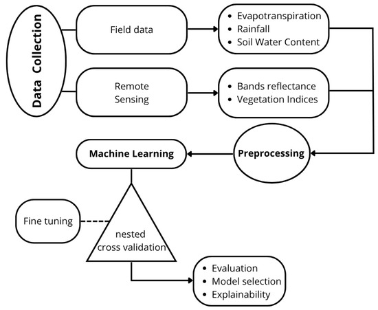
Figure 3.
A flowchart showing the study workflow. The soil water content was considered the target prediction of the machine learning analysis; the evapotranspiration, rainfall, and remote sensing data were used as the predictors.
3.2. Soil Water Content
The observed SWC values across the 0.40 m soil profile exhibited different trends throughout the growing seasons, reflecting the influence of climatic conditions and irrigation events (Figure 4). In 2023, the SWC demonstrated stability, maintaining values of ~145 mm from the beginning of monitoring (6th of June). A gradual rise was observed through the first ten days of July, followed by a subsequent decline until 23rd July, when it reached 126 mm. Thereafter, the trend exhibited variability, characterized by fluctuations in both the increases and decreases, depending on the irrigation and rainfall patterns. In 2024, the SWC exhibited a lower initial value compared to the previous year, starting at approximately 125 mm at the onset of monitoring (27th of June). A moderate increase was recorded during the first days of July, reaching values of ~135 mm. Then, the SWC showed a continuous decline throughout July and the first half of August. Increasing peaks of SWC were observed in the second half of August. From early September, the SWC continued to decrease steadily, with minor fluctuations in the first days of the month. Overall, 2024 was characterized by lower SWC values, a more pronounced and persistent decline, and less pronounced variability compared to 2023.
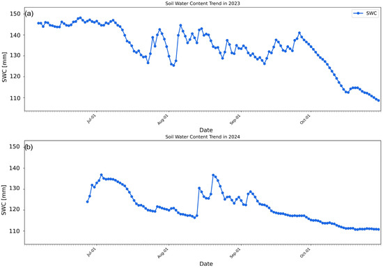
Figure 4.
Soil water content (SWC) of the 0.40 m profile measured within the fields during the two investigated cotton growing seasons of (a) 2023 and (b) 2024.
3.3. Machine Learning Models’ Performance
The comparative performance evaluation of the different machine learning algorithms for SWC prediction is shown in Table 3 and illustrated in Figure 5. The models were compared using the metrics of R2, RMSE, nRMSE, and MBE, calculated by a nested cross-validation. Among all the models tested, the XGBoost showed the best performance, with the highest mean value of R2 (0.734 ± 0.08), the lowest values of RMSE (4.60 ± 0.81 mm) and nRMSE (0.035 ± 0.01), and a low mean MBE error (0.13 ± 0.91). These results are statistically higher than those of the other models, as evidenced by the significant differences shown in Figure 5 (according to the Mann–Whitney U test). In particular, the XGBoost differed markedly from both the linear models (EN and LR) and the other non-linear models (RF, SVR, and KNN) for almost all the metrics, except for the MBE, where the differences were less pronounced. The RF model was the second-best model, with the R2 = 0.601 ± 0.10 and RMSE = 5.69 ± 1.03 mm. The SVR also performed well (R2 = 0.630 ± 0.10; RMSE = 5.43 ± 0.79 mm), but was still lower than the XGBoost (statistically significant differences). The EN, KNN, and LR models showed weaker performances, with the R2 values below 0.60 and higher RMSEs, and generally worse nRMSE and MBE values. The boxplots in Figure 5 confirm these trends, showing greater variability and error distribution in the poorer-performing models. There were highly significant differences between the models for most of the evaluation metrics (p < 0.001 in many cases), except for the MBE, where there was no clear difference between the models. This suggests that the systematic biases were similar across the different algorithms, with the median value around 0.
Table 3.
The performance metrics (with standard deviation, std) calculated using the out-of-fold scores from a nested cross-validation for each model for the prediction of the soil water content: random forest (RF), extreme gradient boosting (XGBoost), elastic net (EN), support vector regression (SVR), k-nearest neighbours (KNN), and linear regression (LR).
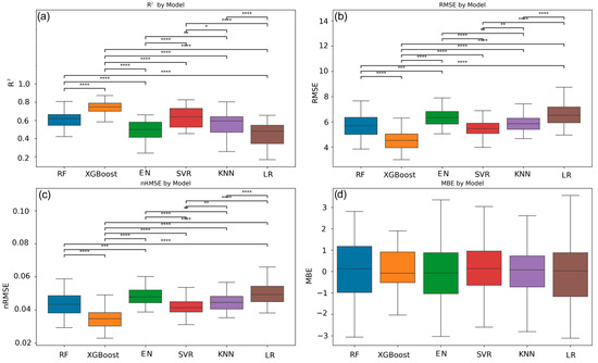
Figure 5.
Model performance comparison for soil water content prediction of the regression algorithms: random forest (RF), extreme gradient boosting (XGBoost), elastic net (EN), support vector regression (SVR), k-nearest neighbours (KNN), and linear regression (LR). The boxplots show the distribution of out-of-fold scores from the nested cross-validation for each model in terms of the following: (a) coefficient of determination (R2); (b) root mean squared error (RMSE); (c) normalized RMSE (nRMSE); and (d) mean bias error (MBE). The central black line represents the median, while the lower and upper boundaries of the box correspond to the first (Q1) and third (Q3) quartiles, respectively. The asterisks indicate statistically significant differences between the models based on the Mann–Whitney U test (* p < 0.05; ** p < 0.01; *** p < 0.001; **** p < 0.0001).
Extreme Gradient Boosting
The XGBoost model demonstrated the best overall performance on SWC estimation, as shown by the cross-model evaluation. Figure 6 illustrates the comparison between the observed and predicted SWC values for XGBoost. The scatterplot shows that the predicted SWC values tend to follow the 1:1 line, with the regression line being close to the bisector. This indicates a generally good agreement between the predictions and observations, despite some residual dispersion.
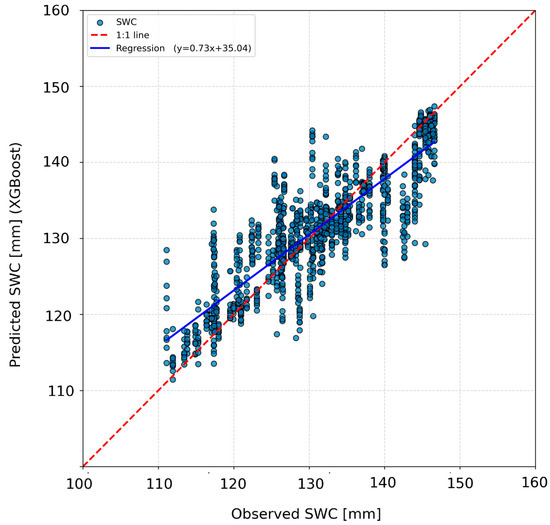
Figure 6.
Scatter plot of cross-validated prediction results for extreme gradient boosting (XGBoost). The x-axis shows the observed soil water content (SWC), while the y-axis reports the predicted SWC values from the model. The red dashed line indicates the 1:1 line (perfect prediction), and the blue line represents the regression fit between the observed and predicted values. The results are based on the out-of-fold predictions from 10 repetitions of the cross-validation.
The residual analysis confirms the performance of XGBoost. Figure 7a shows the distribution of residuals across the observed SWC quartiles. The residual medians in each quartile are close to zero, confirming a reduced systematic bias across the entire SWC. However, there is a slight tendency for positive errors in Q1 and negative errors in Q4, suggesting a marginal overestimation of very low SWC values and a slight underestimation of higher peaks. In Figure 7b, the residuals are grouped by month, and a general tendency is also shown for the error distribution to be centred around zero throughout the growing season. Slight deviations are observed at the beginning and end of the season (June and October), where the residue medians show a slight overestimation at the beginning of the cycle and underestimation at the end of the cycle, respectively.
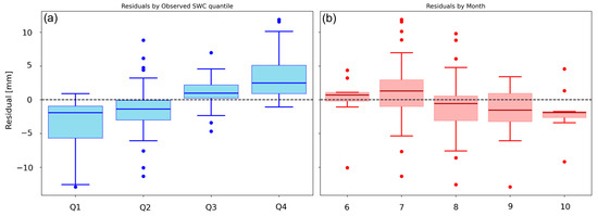
Figure 7.
Boxplots of model residuals (predicted minus observed soil water content, SWC) for the XGBoost model. Residuals grouped by observed SWC quartile (a); residuals grouped by month (June–October) (b). The horizontal dashed line at zero indicates perfect predictions; positive residuals indicate model overestimation, while negative values indicate underestimation.
The feature importance analysis conducted using SHAP provided information on the impact of the predictors on the XGBoost outcomes. Figure 8 shows the percentage contribution of each predictor variable to the model’s decisions. The two agrometeorological variables, the ETo and cumulative rainfall, accounted for over 50% of the total predictive power. The ETo held approximately one-third of the overall importance. Among the remote sensing variables, the NDVI was the most informative (with an importance of 9.9%), followed by the NIR band (6.4%). The contributions of the other spectral indices had lower importances (the NDRE and the PSRI contributed 5.7% and 5.2%, respectively). The reflectance of the other single SDBs and GNDVI had relatively small percentage contributions (less than 5%).
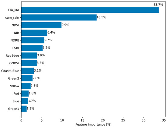
Figure 8.
Feature importance (%) of the predictive variables used by the XGBoost model for the soil water content (SWC) estimation, assessed through a SHapley Additive exPlanations (SHAP) analysis. The bars represent the mean absolute SHAP values aggregated across all predictions, reflecting each feature’s average contribution to the model’s predictions.
4. Discussion
SWC dynamics can be complex, with noise and non-linearity often occurring in the data [39]; therefore, predicting this parameter requires models able to learn from complex patterns and different predictive sources. In this study, XGBoost was found to outperform the other models. This result is in line with the literature; for example, Zhan et al. (2023) [10] used a tree-based gradient boosting to predict the SWC of the Yellow River Delta in Shandong province (China) from Sentinel-2 images. Also, Ren et al. [40] successfully employed XGBoost to predict the soil moisture at the provincial level in China (Jiangsu Province) using meteorological data. In a research work by Zhu et al. [41], conducted in a kiwifruit orchard, XGBoost outperformed the other models in the prediction of soil moisture from multispectral drone images. In general, boosting methods on decision trees have emerged as the most effective for predicting water content dynamics, confirming our results with XGBoost as the top model.
The analysis of the model’s residuals suggests the absence of significant systematic bias, as well as good generalization. Indeed, the medians of the residuals for the SWC quartiles were close to zero, indicating that XGBoost achieved an almost balanced accuracy; however, a greater dispersion of the error was only observed at the extremes of the range, suggesting that the SWC values corresponding to the most exceptional conditions (such as dry soil or the period immediately after heavy rainfall) were more difficult to predict with accuracy. Seasonality also had only a marginal effect on the error. During the summer months, coinciding with blooming and peak crop activity (July–August) [42,43], the variability and bias of residuals remained limited, indicating that the model effectively predicted the SWC dynamics even under high evapotranspirative demand. The slight overestimation at a very low SWC and the underestimation of peaks, as well as the less stable performance in June and October, may reflect both the possible relative scarcity of extreme examples in training and transient conditions (bare soil/early irrigation, autumn rains/senescence), in which the spectral response and agrometeorological drivers varied rapidly. Operationally, these limits could translate into more cautious irrigation activation thresholds when the uncertainty is greater (beginning/end of season). Compared to physical/water balance models (e.g., AquaCrop) and soil/crop process models, the data-driven approach proposed here offers several operational advantages: it requires few explicit soil parameters, natively integrates the near-daily spectral signals and agrometeorological drivers, and can learn non-linear patterns. On the other hand, the absence of physical parameters can generate bias at the extremes of SWC and sensitivity in transient phases; in such cases, hybrid schemes that constrain ML with physical quantities or assimilate the estimated SWC into mechanistic (crop/soil) models can improve the generalization, interpretability, and robustness for out-of-domain conditions, while maintaining the spatiotemporal granularity provided by the near-daily observations.
The SHAP analysis showed the dominant role of agrometeorological information (ETo and cumulative rainfall) on the model predictions, consistent with the fact that the SWC trends are primarily driven by the balance between evaporation and transpiration losses and water inputs [44,45]. Among the remote sensing variables, the NDVI was the main predictive variable. A high NDVI value is often associated with crops that are well supplied with water (then with wetter soils); moreover, a higher NDVI typically reflects a plant’s good physiological status, and one with a high transpiration rate [46,47]. In terms of SHAP importance, the NIR band followed the NDVI. In the early stages of cotton growth, when the plant cover was limited, differences in the bare soil reflectance in the NIR band may have contributed to the model’s performance; in fact, different studies have investigated how the soil moisture content influences the spectral response in the NIR region [48,49,50]. The NDRE and PSRI followed the NIR band in the SHAP analysis. Higher NDRE values tend to correlate with a good water status of a crop, and it is sensitive under water-deficit conditions [51,52]. Conversely, an increase in the PSRI values indicates yellowing and vegetation stress [53]; as water stress increases, plants reduce their photosynthetic activity and exhibit spectral signs of senescence that can be detected by the PSRI. The importance of NIR reflectance and VIs as predictors in the XGBoost model could be due to their strong relationship with a canopy’s physiological status and plant water use. These spectral indicators are proxies for both canopy structural development and physiological activity [54]. A vigorous canopy, indicated by a high NDVI or NDRE and low PSRI, is typically also characterized by an optimal stomatal opening and high rates of transpiration, which result in substantial water fluxes from the soil through the plant to the atmosphere [47]. Moreover, greater canopy cover reduces direct soil evaporation by shading the soil surface, thereby modulating the partitioning between transpiration and evaporation [55]. However, some issues should be considered. While the relationships between the SWC and individual predictors are physiologically consistent, some features of the SHAP results need further consideration. For instance, although the NDVI emerged as an important predictor, its sensitivity to the SWC can be indirectly modulated by other factors, such as nutrient availability, pest pressure, or transient non-water stresses, especially at the canopy closure. This means that, under field conditions, the predictive value of NDVI for soil water may partially reflect confounding factors—not fully captured by the model—that affect the green biomass independently of soil moisture. Additionally, the limited and seasonally variable SHAP importance of PSRI may stem from the relatively short period of true senescence and interannual variability in the onset of stress: in dry summers, plants may show early physiological stress signals (detected in the PSRI) even when the bulk soil moisture is not yet strongly depleted, due to limitations in root exploration or temporary hydraulic disconnection. Moreover, the marginal role of shortwave or blue spectral bands could be reconsidered if future datasets include episodes of surface crusting or rainfall–runoff, which are known to alter soil reflectance and local water retention. Finally, the relatively high importance of ETo reflects the strong atmospheric demand under Mediterranean summers, yet it does not account for the within-field variability in the microclimate or wind exposure, which may explain part of the error variability observed in the residual analysis. Taken together, these aspects highlight the value and limitations of integrating multi-source data for explaining SWC patterns, suggesting that model accuracy could further benefit from the inclusion of additional biotic or pedological variables, or from site-specific calibration in heterogeneous fields. Moreover, in contexts with greater pedological variability and/or with different soil management practices, plot-specific soil characterization would be required to ensure full comparability and model transferability.
From an agronomic point of view, the results of this study may be useful for improving irrigation management and crop monitoring. The restoration of soil hydrological functions (infiltration, storage, and water availability) is an explicitly monitorable objective in regenerative systems; the use of daily SWC estimates fits consistently into this perspective as an operational indicator for comparative assessments and irrigation decision support [56]. The calibration of the model does not require laboratory analyses but only the installation of capacitive probes in the soil, making the approach practical and cost-effective for farmers. Furthermore, the model can be recalibrated each season. A data-driven model able to estimate the SWC on a daily basis could help to optimize irrigation decisions in near real time. In operational terms, daily SWC estimates could be converted to root zone depletion (Dr) and compared with the readily available water (RAW); irrigation could be started to restore the SWC to close to field capacity, with specific thresholds for each stage that are more conservative during the critical mid-season stage of cotton (from flowering to boll development) and more permissive in less sensitive phases, thus aligning the timing and doses with crop water requirements while remaining in line with the FAO-56 programming principle [31].
In the context of regenerative and conservative farming or cultivation under semi-arid conditions—characterized by agronomic practices that improve soil health and the water retention capacity, such as cover crops and reduced tillage [57,58]—a predictive SWC model may help to prevent crop water stress and reduce water input. Moreover, unlike approaches based on fixed thresholds or predetermined irrigation calendars, a predictive model that integrates agrometeorological and satellite data reflects the specific water–physiological response of a soil–plant–atmosphere system, thus providing more dynamic and adaptive decision support, especially if used in combination with information on the canopy’s water status (e.g., stem water potential) [9]. Farmers and technicians can use daily SWC estimates to identify the optimal timing of irrigation, adjusting interventions according to the predicted SWC. Another advantage of this approach is the use of high-frequency satellite data. The SuperDove constellation provides near-daily images, enabling almost continuous monitoring of SWC. Other satellite platforms, such as Sentinel-2 and Landsat, have a lower acquisition frequency, which limits the practical application of models for real-time irrigation management compared to SuperDove [10].
However, it is necessary to highlight some limitations of the proposed framework. Although the use of near-daily Planet SuperDove imagery significantly increases the temporal resolution, clouds, especially during certain crop stages or weather events, can still result in data gaps. In this study, model training was based only on cloud-free observations, excluding days with unavailable or contaminated imagery. Therefore, there may be limitations in the model’s reliability when satellite data are unavailable for extended periods. This also limits the operational use of the model during periods of persistent cloudiness, potentially reducing its prediction reliability or temporal continuity. Future work should address this issue by testing data gap-filling techniques, such as temporal interpolation, data fusion with other sensors, or including methods to quantify and propagate satellite data uncertainty into model outputs.
The model predictions are specifically fitted to the homogeneous management area in which the calibration data (i.e., the SWC) were collected. Therefore, the framework is mainly applicable to homogeneous fields or farms, and its applicability would decrease in heterogeneous fields. Thus, in the case of heterogeneity, multiple zones would require multiple calibrations to ensure that the predicted SWC values remain representative; this approach would follow standard agronomic practices, given that soil properties and growing conditions can vary between zones [59,60]. In this context, the VIs could also help to identify homogeneous areas [61]. Future research could exploit the spatial dimension of Planet imagery to generate high-resolution SWC distribution maps of larger or heterogeneous farms, where the sub-field variability requires site-specific irrigation management. Also, model accuracy could potentially be further improved by exploring additional or alternative indices that may offer greater sensitivity to particular stress signals or stages of canopy development. Feature engineering or data-driven selection of VI combinations—using techniques like recursive feature elimination, automated variable selection, or advanced spectral transformations—could enhance the model’s predictive power. Future research in this direction could systematically evaluate a broader range of VIs, adapting the VIs to crop phenology, growth stage, and specific stress conditions, in order to maximize the model’s ability to generalize and capture complex soil–plant–atmosphere interactions.
5. Conclusions
This study reported the results of an integration of agrometeorological and satellite data for building an ML framework to predict the SWC in cotton cultivation. Among the compared ML models, XGBoost achieved the best predictive performance (R2 = 0.73 ± 0.008) and lowest error (nRMSE = 0.035 ± 0.01). The SHAP analysis revealed that the agrometeorological variables, such as the ETo and cumulative rainfall, had a high impact on model performance, while the spectral data (e.g., NDVI, NIR band, NDRE, and PSRI) provided complementary information. This work demonstrates the usefulness and potential of integrating high-frequency and high-resolution satellite products with explainable AI techniques.
From an agronomic point of view, the developed framework could be applicable at the farm or sub-farm scale, with potential for use in site-specific irrigation-optimization decision-making systems. The integration of this approach with automated data acquisition systems and digital platforms could also be tested to facilitate its wider adoption. Finally, combining satellite-based machine learning models with physics-based crop models or advanced sensor networks could improve the interpretability and reliability of SWC predictions in different agricultural scenarios and setups.
Author Contributions
Conceptualization, S.P.G. and P.C.; Data curation, S.P.G., A.F.M. and N.S.; Formal analysis, S.P.G.; Funding acquisition, G.S.M.; Investigation, S.P.G., A.F.M., N.S. and M.N.T.; Methodology, S.P.G. and P.C.; Project administration, G.S.M. and P.C.; Resources, P.C.; Software, S.P.G. and P.C.; Supervision, A.F.M. and P.C.; Validation, P.C.; Visualization, S.P.G.; Writing—original draft, S.P.G.; Writing—review and editing, G.S.M., A.F.M., N.S., M.N.T. and P.C. All authors have read and agreed to the published version of the manuscript.
Funding
This work was funded by the Apulia Regenerative Cotton project (Project: PRJ00039) coordinated by the European Forest Institute.
Institutional Review Board Statement
Not applicable.
Informed Consent Statement
Not applicable.
Data Availability Statement
The original contributions presented in this study are included in the article. Further inquiries can be directed to the corresponding author.
Acknowledgments
The authors thank Armani Group for the funding provided to establish the Apulia Agroforestry Regenerative Cotton Project as a Living Lab of the Circular Bioeconomy Alliance, within its partnership with the Sustainable Markets Initiative’s Fashion Task Force.
Conflicts of Interest
The authors declare that there are no conflicts of interest regarding the publication of this article.
References
- Biswas, A.; Sarkar, S.; Das, S.; Dutta, S.; Roy Choudhury, M.; Giri, A.; Bera, B.; Bag, K.; Mukherjee, B.; Banerjee, K.; et al. Water Scarcity: A Global Hindrance to Sustainable Development and Agricultural Production—A Critical Review of the Impacts and Adaptation Strategies. Camb. Prism. Water 2025, 3, e4. [Google Scholar] [CrossRef]
- Yang, P.; Wu, L.; Cheng, M.; Fan, J.; Li, S.; Wang, H.; Qian, L. Review on Drip Irrigation: Impact on Crop Yield, Quality, and Water Productivity in China. Water 2023, 15, 1733. [Google Scholar] [CrossRef]
- Negash, M.; Tegegne, Y.T.; Palahi, M.; Valter, Z.; Garofalo, S.P.; De Carolis, G.; Campi, P.; Modugno, A.F.; Scarascia-Mugnozza, G. Overview of Regenerative and Agroforestry-Based Cotton Systems in the Mediterranean and beyond: A Review. Agrofor. Syst. 2025, 99, 117. [Google Scholar] [CrossRef]
- Khangura, R.; Ferris, D.; Wagg, C.; Bowyer, J. Regenerative Agriculture—A Literature Review on the Practices and Mechanisms Used to Improve Soil Health. Sustainability 2023, 15, 2338. [Google Scholar] [CrossRef]
- Maldera, F.; Garofalo, S.P.; Camposeo, S. Ecophysiological Recovery of Micropropagated Olive Cultivars: Field Research in an Irrigated Super-High-Density Orchard. Agronomy 2024, 14, 1560. [Google Scholar] [CrossRef]
- Istanbulluoglu, A. Effects of Irrigation Regimes on Yield and Water Productivity of Safflower (Carthamus tinctorius L.) under Mediterranean Climatic Conditions. Agric. Water Manag. 2009, 96, 1792–1798. [Google Scholar] [CrossRef]
- Iglesias, A.; Garrote, L.; Flores, F.; Moneo, M. Challenges to Manage the Risk of Water Scarcity and Climate Change in the Mediterranean. Water Resour. Manag. 2007, 21, 775–788. [Google Scholar] [CrossRef]
- García-Ruiz, J.M.; López-Moreno, I.I.; Vicente-Serrano, S.M.; Lasanta-Martínez, T.; Beguería, S. Mediterranean Water Resources in a Global Change Scenario. Earth Sci. Rev. 2011, 105, 121–139. [Google Scholar] [CrossRef]
- Garofalo, S.P.; Modugno, A.F.; De Carolis, G.; Sanitate, N.; Negash Tesemma, M.; Scarascia-Mugnozza, G.; Tekle Tegegne, Y.; Campi, P. Explainable Artificial Intelligence to Predict the Water Status of Cotton (Gossypium hirsutum L., 1763) from Sentinel-2 Images in the Mediterranean Area. Plants 2024, 13, 3325. [Google Scholar] [CrossRef]
- Zhan, D.; Mu, Y.; Duan, W.; Ye, M.; Song, Y.; Song, Z.; Yao, K.; Sun, D.; Ding, Z. Spatial Prediction and Mapping of Soil Water Content by TPE-GBDT Model in Chinese Coastal Delta Farmland with Sentinel-2 Remote Sensing Data. Agriculture 2023, 13, 1088. [Google Scholar] [CrossRef]
- Lee, H.; Wang, J.; Leblon, B. Using Linear Regression, Random Forests, and Support Vector Machine with Unmanned Aerial Vehicle Multispectral Images to Predict Canopy Nitrogen Weight in Corn. Remote Sens. 2020, 12, 2071. [Google Scholar] [CrossRef]
- Lin, Y.; Zhu, Z.; Guo, W.; Sun, Y.; Yang, X.; Kovalskyy, V. Continuous Monitoring of Cotton Stem Water Potential Using Sentinel-2 Imagery. Remote Sens. 2020, 12, 1176. [Google Scholar] [CrossRef]
- Campi, P.; Modugno, A.F.; De Carolis, G.; Pedrero Salcedo, F.; Lorente, B.; Garofalo, S. Pietro A Machine Learning Approach to Monitor the Physiological and Water Status of an Irrigated Peach Orchard under Semi-Arid Conditions by Using Multispectral Satellite Data. Water 2024, 16, 2224. [Google Scholar] [CrossRef]
- López-Andreu, F.J.; López-Morales, J.A.; Erena, M.; Skarmeta, A.F.; Martínez, J.A. Monitoring System for the Management of the Common Agricultural Policy Using Machine Learning and Remote Sensing. Electronics 2022, 11, 325. [Google Scholar] [CrossRef]
- Hassan-Esfahani, L.; Torres-Rua, A.; McKee, M. Assessment of Optimal Irrigation Water Allocation for Pressurized Irrigation System Using Water Balance Approach, Learning Machines, and Remotely Sensed Data. Agric. Water Manag. 2015, 153, 42–50. [Google Scholar] [CrossRef]
- Wei, S.; Xu, T.; Niu, G.Y.; Zeng, R. Estimating Irrigation Water Consumption Using Machine Learning and Remote Sensing Data in Kansas High Plains. Remote Sens. 2022, 14, 3004. [Google Scholar] [CrossRef]
- Garofalo, S.P.; Giannico, V.; Lorente, B.; García, A.J.G.; Vivaldi, G.A.; Thameur, A.; Salcedo, F.P. Predicting Carob Tree Physiological Parameters under Different Irrigation Systems Using Random Forest and Planet Satellite Images. Front. Plant Sci. 2024, 15, 1302435. [Google Scholar] [CrossRef] [PubMed]
- Jenkins, M.; Block, D.E. A Review of Methods for Data-Driven Irrigation in Modern Agricultural Systems. Agronomy 2024, 14, 1355. [Google Scholar] [CrossRef]
- Segarra, J.; Buchaillot, M.L.; Araus, J.L.; Kefauver, S.C. Remote Sensing for Precision Agriculture: Sentinel-2 Improved Features and Applications. Agronomy 2020, 10, 641. [Google Scholar] [CrossRef]
- Carminati, A.; Moradi, A.B.; Vetterlein, D.; Vontobel, P.; Lehmann, E.; Weller, U.; Vogel, H.J.; Oswald, S.E. Dynamics of Soil Water Content in the Rhizosphere. Plant Soil. 2010, 332, 163–176. [Google Scholar] [CrossRef]
- Campi, P.; Gaeta, L.; Mastrorilli, M.; Losciale, P. Innovative Soil Management and Micro-Climate Modulation for Saving Water in Peach Orchards. Front. Plant Sci. 2020, 11, 544947. [Google Scholar] [CrossRef]
- Specifications|Observatory—SMAP. Available online: https://smap.jpl.nasa.gov/observatory/specifications/ (accessed on 8 July 2025).
- SMOS—Earth Online. Available online: https://earth.esa.int/eogateway/missions/smos#instruments-section (accessed on 8 July 2025).
- Sharma, A.; Jain, A.; Gupta, P.; Chowdary, V. Machine Learning Applications for Precision Agriculture: A Comprehensive Review. IEEE Access 2021, 9, 4843–4873. [Google Scholar] [CrossRef]
- Ahmad, S.; Kalra, A.; Stephen, H. Estimating Soil Moisture Using Remote Sensing Data: A Machine Learning Approach. Adv. Water Resour. 2010, 33, 69–80. [Google Scholar] [CrossRef]
- Rani, A.; Kumar, N.; Kumar, J.; Sinha, N.K. Machine Learning for Soil Moisture Assessment. In Deep Learning for Sustainable Agriculture; Academic Press: Cambridge, MA, USA, 2022; pp. 143–168. [Google Scholar] [CrossRef]
- Mehmeti, A.; Abdelhafez, A.A.M.; Ellssel, P.; Todorovic, M.; Calabrese, G. Performance and Sustainability of Organic and Conventional Cotton Farming Systems in Egypt: An Environmental and Energy Assessment. Sustainability 2024, 16, 6637. [Google Scholar] [CrossRef]
- Zhang, Z.; Huang, J.; Yao, Y.; Peters, G.; Macdonald, B.; La Rosa, A.D.; Wang, Z.; Scherer, L. Environmental Impacts of Cotton and Opportunities for Improvement. Nat. Rev. Earth Environ. 2023, 4, 703–715. [Google Scholar] [CrossRef]
- Naderi Mahdei, K.; Esfahani, S.M.J.; Lebailly, P.; Dogot, T.; Van Passel, S.; Azadi, H. Environmental Impact Assessment and Efficiency of Cotton: The Case of Northeast Iran. Environ. Dev. Sustain. 2023, 25, 10301–10321. [Google Scholar] [CrossRef]
- Garofalo, S.P.; Modugno, A.F.; de Carolis, G.; Campi, P. Energy of Sorghum Biomass Under Deficit Irrigation Strategies in the Mediterranean Area. Water 2025, 17, 578. [Google Scholar] [CrossRef]
- Allen, R.G.; Pereira, L.S.; Raes, D.; Smith, M. Crop Evapotranspiration-Guidelines for Computing Crop Water Requirements—FAO Irrigation and Drainage Paper 56; FAO: Rome, Italy, 1998; p. 300. [Google Scholar]
- Gitelson, A.; Merzlyak, M.N. Quantitative Estimation of Chlorophyll-a Using Reflectance Spectra: Experiments with Autumn Chestnut and Maple Leaves. J. Photochem. Photobiol. B 1994, 22, 247–252. [Google Scholar] [CrossRef]
- Rouse, J.W.; Haas, R.H.; Schell, J.A.; Deering, D.W. Monitoring Vegetation Systems in the Great Plains with ERTS. In Proceedings of the Third Earth Resources Technology Satellite-1 Symposium, Washington, DC, USA, 10–14 December 1973; p. 309. [Google Scholar]
- Nunes, P.H.; Pierangeli, E.V.; Santos, M.O.; Silveira, H.R.O.; de Matos, C.S.M.; Pereira, A.B.; Alves, H.M.R.; Volpato, M.M.L.; Silva, V.A.; Ferreira, D.D. Predicting Coffee Water Potential from Spectral Reflectance Indices with Neural Networks. Smart Agric. Technol. 2023, 4, 100213. [Google Scholar] [CrossRef]
- Gitelson; Kaufman, Y.J.; Merzlyak, M.N. Use of a Green Channel in Remote Sensing of Global Vegetation from EOS-MODIS. Remote Sens. Environ. 1996, 58, 289–298. [Google Scholar] [CrossRef]
- Pedregosa, F.; Michel, V.; Grisel, O.; Blondel, M.; Prettenhofer, P.; Weiss, R.; Vanderplas, J.; Cournapeau, D.; Pedregosa, F.; Varoquaux, G.; et al. Scikit-Learn: Machine Learning in Python. J. Mach. Learn. Res. 2011, 12, 2825–2830. [Google Scholar]
- Chen, T.; Guestrin, C. XGBoost: A Scalable Tree Boosting System. In Proceedings of the ACM SIGKDD International Conference on Knowledge Discovery and Data Mining, San Francisco, CA, USA, 13–17 August 2016; pp. 785–794. [Google Scholar] [CrossRef]
- Nested Versus Non-Nested Cross-Validation. Scikit-Learn 1.7.0 Documentation. Available online: https://scikit-learn.org/stable/auto_examples/model_selection/plot_nested_cross_validation_iris.html (accessed on 17 July 2025).
- Li, P.; Zha, Y.; Shi, L.; Tso, C.H.M.; Zhang, Y.; Zeng, W. Comparison of the Use of a Physical-Based Model with Data Assimilation and Machine Learning Methods for Simulating Soil Water Dynamics. J Hydrol. 2020, 584, 124692. [Google Scholar] [CrossRef]
- Ren, Y.; Ling, F.; Wang, Y. Research on Provincial-Level Soil Moisture Prediction Based on Extreme Gradient Boosting Model. Agriculture 2023, 13, 927. [Google Scholar] [CrossRef]
- Zhu, S.; Cui, N.; Guo, L.; Jin, H.; Jin, X.; Jiang, S.; Wu, Z.; Lv, M.; Chen, F.; Liu, Q.; et al. Enhancing Precision of Root-Zone Soil Moisture Content Prediction in a Kiwifruit Orchard Using UAV Multi-Spectral Image Features and Ensemble Learning. Comput. Electron. Agric. 2024, 221, 108943. [Google Scholar] [CrossRef]
- Zafar, S.; Afzal, H.; Ijaz, A.; Mahmood, A.; Ayub, A.; Nayab, A.; Hussain, S.; UL-Hussan, M.; Sabir, M.A.; Zulfiqar, U.; et al. Cotton and Drought Stress: An Updated Overview for Improving Stress Tolerance. South. Afr. J. Bot. 2023, 161, 258–268. [Google Scholar] [CrossRef]
- Ul-Allah, S.; Rehman, A.; Hussain, M.; Farooq, M. Fiber Yield and Quality in Cotton under Drought: Effects and Management. Agric. Water Manag. 2021, 255, 106994. [Google Scholar] [CrossRef]
- Seneviratne, S.I.; Corti, T.; Davin, E.L.; Hirschi, M.; Jaeger, E.B.; Lehner, I.; Orlowsky, B.; Teuling, A.J. Investigating Soil Moisture–Climate Interactions in a Changing Climate: A Review. Earth Sci. Rev. 2010, 99, 125–161. [Google Scholar] [CrossRef]
- Babaeian, E.; Sadeghi, M.; Jones, S.B.; Montzka, C.; Vereecken, H.; Tuller, M. Ground, Proximal, and Satellite Remote Sensing of Soil Moisture. Rev. Geophys. 2019, 57, 530–616. [Google Scholar] [CrossRef]
- Stamford, J.D.; Vialet-Chabrand, S.; Cameron, I.; Lawson, T. Development of an Accurate Low Cost NDVI Imaging System for Assessing Plant Health. Plant Methods 2023, 19, 1–19. [Google Scholar] [CrossRef]
- Jones, H.G. Plants and Microclimate: A Quantitative Approach to Environmental Plant Physiology; Cambridge University Press (CUP): Cambridge, UK, 2013; pp. 1–407. ISBN 9780521279598. [Google Scholar] [CrossRef]
- Loshelder, J.I.; Coffman, R.A. Soil Moisture Content from Spectral Reflectance Using Visible, Near-Infrared, and Short-Wave Infrared Light. J. Irrig. Drain. Eng. 2023, 149, 04023010. [Google Scholar] [CrossRef]
- Jiang, Q.; Chen, Y.; Guo, L.; Fei, T.; Qi, K. Estimating Soil Organic Carbon of Cropland Soil at Different Levels of Soil Moisture Using VIS-NIR Spectroscopy. Remote Sens. 2016, 8, 755. [Google Scholar] [CrossRef]
- Whiting, M.L.; Li, L.; Ustin, S.L. Predicting Water Content Using Gaussian Model on Soil Spectra. Remote Sens. Environ. 2004, 89, 535–552. [Google Scholar] [CrossRef]
- Yang, M.; Hassan, M.A.; Xu, K.; Zheng, C.; Rasheed, A.; Zhang, Y.; Jin, X.; Xia, X.; Xiao, Y.; He, Z. Assessment of Water and Nitrogen Use Efficiencies Through UAV-Based Multispectral Phenotyping in Winter Wheat. Front. Plant Sci. 2020, 11, 537910. [Google Scholar] [CrossRef]
- Tang, Z.; Jin, Y.; Alsina, M.M.; McElrone, A.J.; Bambach, N.; Kustas, W.P. Vine Water Status Mapping with Multispectral UAV Imagery and Machine Learning. Irrig. Sci. 2022, 40, 715–730. [Google Scholar] [CrossRef]
- Anderegg, J.; Yu, K.; Aasen, H.; Walter, A.; Liebisch, F.; Hund, A. Spectral Vegetation Indices to Track Senescence Dynamics in Diverse Wheat Germplasm. Front. Plant Sci. 2020, 10, 466315. [Google Scholar] [CrossRef] [PubMed]
- Gitelson, A.A.; Merzlyak, M.N. Remote Sensing of Chlorophyll Concentration in Higher Plant Leaves. Adv. Space Res. 1998, 22, 689–692. [Google Scholar] [CrossRef]
- O’donoghue, T.; Minasny, B.; McBratney, A. Regenerative Agriculture and Its Potential to Improve Farmscape Function. Sustainability 2022, 14, 5815. [Google Scholar] [CrossRef]
- Soto, R.L.; Martínez-Mena, M.; Padilla, M.C.; de Vente, J. Restoring soil quality of woody agroecosystems in Mediterranean drylands through regenerative agriculture. Agric. Ecosyst. Environ. 2021, 306, 107191. [Google Scholar] [CrossRef]
- Alharbi, S.; Felemban, A.; Abdelrahim, A.; Al-Dakhil, M. Agricultural and Technology-Based Strategies to Improve Water-Use Efficiency in Arid and Semiarid Areas. Water 2024, 16, 1842. [Google Scholar] [CrossRef]
- Thapa, V.R.; Ghimire, R.; Adhikari, K.P.; Lamichhane, S. Soil Organic Carbon Sequestration Potential of Conservation Agriculture in Arid and Semi-Arid Regions: A Review. J. Arid. Environ. 2023, 217, 105028. [Google Scholar] [CrossRef]
- Yetbarek, E.; Kumar, S.; Ojha, R. Effects of Soil Heterogeneity on Subsurface Water Movement in Agricultural Fields: A Numerical Study. J. Hydrol. 2020, 590, 125420. [Google Scholar] [CrossRef]
- Tittonell, P.; Vanlauwe, B.; de Ridder, N.; Giller, K.E. Heterogeneity of Crop Productivity and Resource Use Efficiency within Smallholder Kenyan Farms: Soil Fertility Gradients or Management Intensity Gradients? Agric. Syst. 2007, 94, 376–390. [Google Scholar] [CrossRef]
- Oldoni, H.; Costa, B.R.S.; Bognola, I.A.; de Souza, C.R.; Bassoi, L.H. Homogeneous Zones of Vegetation Index for Characterizing Variability and Site-Specific Management in Vineyards. Sci. Agric. 2020, 78, e20190243. [Google Scholar] [CrossRef]
Disclaimer/Publisher’s Note: The statements, opinions and data contained in all publications are solely those of the individual author(s) and contributor(s) and not of MDPI and/or the editor(s). MDPI and/or the editor(s) disclaim responsibility for any injury to people or property resulting from any ideas, methods, instructions or products referred to in the content. |
© 2025 by the authors. Licensee MDPI, Basel, Switzerland. This article is an open access article distributed under the terms and conditions of the Creative Commons Attribution (CC BY) license (https://creativecommons.org/licenses/by/4.0/).