Abstract
Coal is a vital part of China’s energy system, and accurately predicting mine water inflow is crucial for ensuring the safety and efficiency of coal mining. To enhance prediction accuracy, this study introduces a hybrid model—CEEMDAN-OVMD-Transformer—that combines Adaptive Noise Complete Ensemble Empirical Mode Decomposition (CEEMDAN), Optimal Variational Mode Decomposition (OVMD), and the Transformer architecture. This combined model is used to forecast water inflow at the Heidaigou Coal Mine. The experimental results show that the proposed model achieves excellent predictive accuracy, with a Mean Absolute Error (MAE) of 0.507, a Root Mean Square Error (RMSE) of 0.614, a Mean Absolute Percentage Error (MAPE) of 0.010, and a Coefficient of Determination (R2) of 0.948. Compared to the standalone Transformer model, the CEEMDAN-OVMD-Transformer model reduces the MAE by 34.50% and increases the R2 by approximately 3.04%, indicating a significant improvement in forecasting accuracy. The findings demonstrate that the CEEMDAN-OVMD-Transformer hybrid model can effectively reduce the complexity of high-frequency components in mine water inflow time series, thereby enhancing the stability and reliability of predictions. This research presents a new and effective approach for mine water inflow forecasting and offers valuable technical guidance for water hazard prevention and control in similar coal mining environments.
1. Introduction
In the mining industry, accurate prediction of mine water inflow is essential for ensuring safety and optimizing drainage system design [1,2]. Precise characterization of water inflow trends provides vital support for mine planning and hazard mitigation strategies. However, mine water inflow is affected by many complex factors, including geological structures, weather conditions, and mining activities [3,4]. The interaction of these variables creates significant non-stationarity and inherent complexity in water inflow time series, increasing the difficulty of predictive modeling. Conventional methods, such as analytical techniques and hydrogeological analogy approaches [5,6], mainly rely on empirical formulas and simplified geological models, which often fail to capture the complexities of real-world conditions. These methods frequently lack adequate predictive accuracy when dealing with intricate geological formations and variable influencing factors, potentially threatening safety standards. With advances in data-driven techniques, machine learning and deep learning methods are increasingly employed for mine water inflow forecasting. Nevertheless, traditional models like support vector machines and basic neural networks [7,8] encounter difficulties with processing long-term sequences and recognizing complex dependency patterns, limiting their capacity to fully extract valuable features from water inflow data [9,10].
With advances in deep learning algorithms, various methods have been applied to research on mine water inflow prediction. For example, Liu et al. [11] developed a TCN-LSTM-SVM model to forecast mine water inflow in the Binchang Mining Area of Shaanxi Province. The accuracy of this model exceeds that of models like BP neural networks and random forests, making it practically useful for predicting water inflow and guiding water prevention and control efforts in mines with similar geological conditions. Zhao et al. [7] introduced a Bi-RNN combined with a GMS model for predicting surface mine water inflow at the Shabaosi Gold Mine in Mohe City, Heilongjiang Province. This approach demonstrates advantages over traditional techniques such as the large well method and the recharge modulus large well method.
In recent years, the Transformer model has achieved notable breakthroughs in fields like natural language processing and computer vision. Its powerful self-attention mechanism enables it to effectively capture long-range dependencies, demonstrating advantages in time-series prediction tasks. Compared to traditional recurrent neural networks (RNNs) and their variants, the Transformer employs a multi-head attention mechanism to compute relationships between sequence elements simultaneously, avoiding issues like gradient vanishing and explosion. This allows it to process long-sequence data more efficiently and improves prediction accuracy. When handling long-span mine water inflow data, the Transformer can fully exploit the potential relationships between data points at different times, providing reliable support for accurate forecasts [12,13].
Single prediction models often struggle to precisely forecast non-stationary monthly runoff time series. Modal decomposition methods, such as wavelet decomposition (WD), empirical mode decomposition (EMD), and variational mode decomposition (VMD), are effective for dealing with non-stationary signals and are widely used in data preprocessing [14,15,16]. In managing non-stationary signals, CEEMDAN and OVMD have demonstrated outstanding performance. CEEMDAN introduces adaptive white noise based on EMD, effectively resolving the mode mixing problem and accurately decomposing complex original signals into multiple intrinsic mode function (IMF) components with distinct frequency characteristics. This makes each component more regular and easier to analyze, thus providing better data features for subsequent prediction models.
Therefore, the CEEMDAN, OVMD, and Transformer are combined to develop the CEEMDAN-OVMD-Transformer model for mine water inflow prediction. Through case analysis, this model’s predictive performance is thoroughly assessed and compared with other common prediction models to highlight its advantages and applicability. The goal is to provide a more effective method for mine water inflow prediction, offer more reliable technical support for mine safety and resource utilization, and promote the sustainable development of the mining industry.
2. Principles of the Prediction Model Based on Empirical Mode Decomposition and Transformer
2.1. Principle of Complete Ensemble Empirical Mode Decomposition with Adaptive Noise
EMD is an adaptive signal processing method primarily used for handling nonlinear and non-stationary signals. It can decompose complex signals into a series of IMFs. However, traditional EMD methods have certain limitations when dealing with noisy signals. CEEMDAN is developed based on EMD and EEMD, which can more effectively suppress noise and improve decomposition accuracy [17,18].
The principle of CEEMDAN is illustrated in Figure 1 below, with the specific steps as follows:
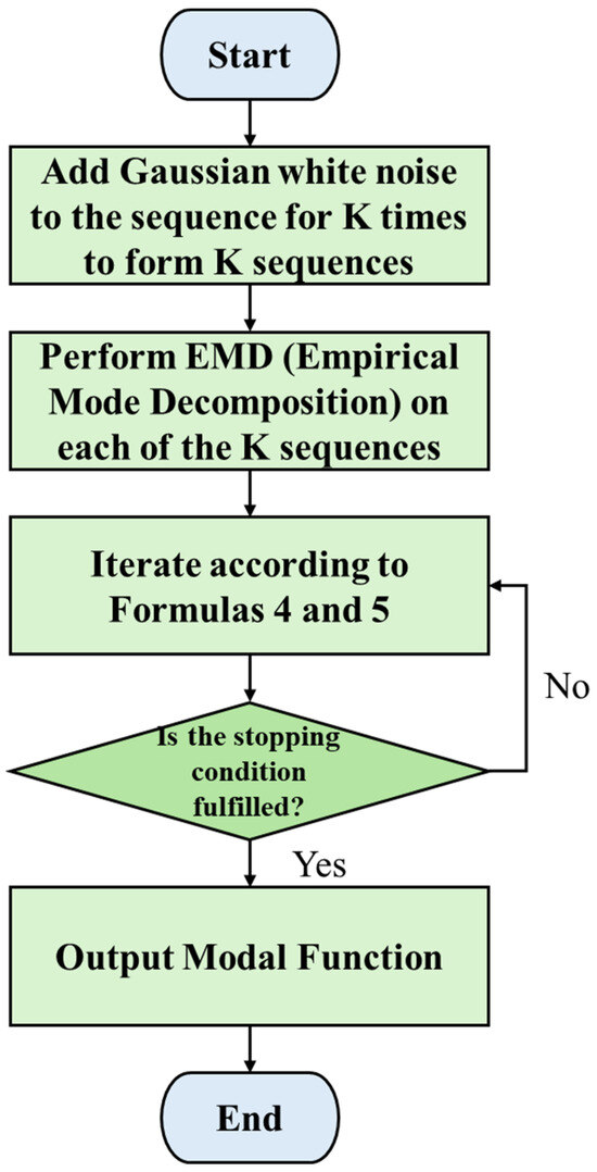
Figure 1.
CEEMDAN Principle.
Step 1: First, add white noise with different amplitudes to the original data to construct a noisy sequence , as shown in the formula below:
where is the noise amplitude coefficient, is the white noise added at the -th time, is the number of times white noise is added, and represents different time nodes.
Step 2: Define as the -th component after EMD. Perform EMD on the generated sequences to obtain the first intrinsic mode function . The first intrinsic mode component of CEEMDAN is obtained by calculating the average of the first intrinsic mode functions:
The first residual is:
Step 3: Add white noise to the residual to obtain a new sequence , and perform EMD to obtain the second intrinsic mode component :
The second residual is:
Step 4: Repeat Step 3, adding white noise before each decomposition. After k decompositions, the k-th component is obtained, as shown in Formulas (6) and (7).
Step 5: If the residual signal after the n-th decomposition is a monotonic signal, the iteration stops, and the CEEMDAN algorithm decomposition ends. The original water inflow sequence can be expressed as:
2.2. Optimal Variational Mode Decomposition
OVMD is an enhanced signal decomposition method derived from VMD. It effectively handles non-stationary and nonlinear signals and is widely applied across multiple disciplines. Its core principle relies on variational methods and the center frequency approach to determine the number of decomposition layers, as explained below:
Variational Model Construction: OVMD firstly decomposes the original signal into K mode functions with limited bandwidth. Each mode function is subjected to a Hilbert transform to obtain an analytic signal, and its spectrum is shifted to the baseband. The center frequency is estimated to determine the signal bandwidth. A variational model is constructed to minimize the sum of the estimated bandwidths of each modal function while ensuring that the sum of all mode functions equals the original signal:
where and are the sets of the k-th modal component and center frequency after decomposition, respectively, is the impulse function, is the imaginary unit, is the modal function, is the number of modes obtained from decomposition, and tt is the number of sampling points.
Augmented Lagrangian Function Transformation: Introduce the Lagrange multiplier and the quadratic penalty factor to transform the constrained variational problem into an augmented Lagrangian function, as shown in the formula below:
This transformation allows the use of iterative algorithms to solve the variational problem, making the solution process more efficient and stable.
Iterative Update of Mode Components and Center Frequencies: Use the Alternating Direction Method of Multipliers to iteratively update the intrinsic mode components and center frequencies. The update formulas are:
where ,, are the Fourier transforms of ,,. Through continuous iteration, the mode components and center frequencies gradually reach the optimal solution.
Determining the Number of Decomposition Layers: This is a key improvement in OVMD. It uses the center frequency method to identify how many decomposition layers are needed, calculating the update step size based on the minimum error index. During the iterative process, different numbers of layers are tested, and the corresponding error indices are recorded. The number of layers with the smallest error index is chosen as the final result. This approach removes the subjectivity of manually selecting the number of layers and can adaptively find the optimal number based on the signal’s characteristics, more accurately capturing the nonlinear features of the time series.
2.3. Principle of the Transformer Model
The Transformer is a deep learning architecture based on the self-attention mechanism, introduced by Vaswani et al. [19] from Google in the paper “Attention is All You Need” in 2017, and used for natural language processing. Because of its excellent performance in language sequences, it has increasingly been applied to solve more time series tasks in recent years. The main idea of the Transformer is to capture long-distance dependencies in sequence data through the self-attention mechanism while enhancing processing efficiency with parallel computation.
The core architecture of the Transformer model consists of an encoder and a decoder [19].
The left box in Figure 2 shows the Transformer’s encoder, which is made up of multiple identical EncoderLayer blocks stacked together. Each layer features two main parts: a multi-head self-attention module and a feed-forward neural network equipped with a ReLU activation. The output from each EncoderLayer goes through residual connections and layer normalization (Add & Norm) to avoid gradient vanishing and speed up training.
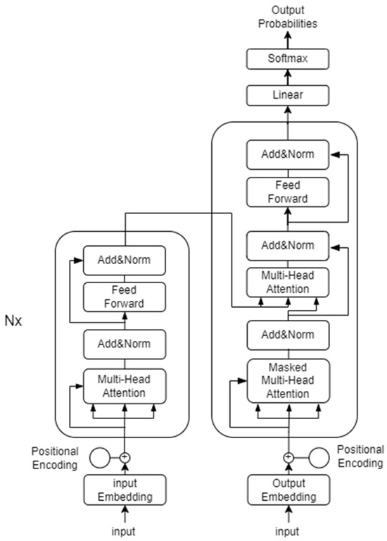
Figure 2.
Transformer Model Structure.
The self-attention mechanism is the core of the Transformer. The principle of the self-attention mechanism is shown in Figure 3.
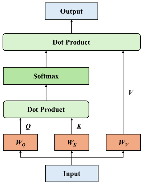
Figure 3.
Self-Attention Mechanism Diagram.
Since the self-attention mechanism does not have inherent sequence order information like RNNs, position encoding is essential to provide the model with positional context. Position encoding typically uses sine and cosine functions.
where is the position of the data, is the dimension index, and is the dimension of the Transformer. For the input sequence , the embedding matrix is added to the position encoding to form the input matrix , which is then multiplied by the query , key and value matrices to obtain , , .
The vector is used to obtain information, the vector is used to mark important parts of the data, and the vector contains the actual information. The similarity between and is measured by the dot product, and the relationship weights are calculated using the Softmax function, which is then multiplied by the vector to obtain the output of the single-head attention mechanism .
where is the dimension of the key vector, preventing the dot product result from becoming too large and causing the Softmax gradient to vanish.
This model uses a multi-head self-attention mechanism, where outputs from multiple single-head attentions are combined to create the final multi-head self-attention output. Residual connections and layer normalization (Add & Norm) are used to reduce gradient vanishing problems and speed up training. The formula is as follows:
Encoder: First, it captures long-range dependencies in sequential data through a multi-head self-attention mechanism. It also utilizes a feedforward neural network to enhance the model’s nonlinear expressive capabilities and further extract features. The computational formula is:
The time series data processed by the encoder can include rich, multi-dimensional information, which aids in more detailed data analysis and prediction.
Decoder: Similar in structure to the encoder, the decoder employs a Masked Multi-Head Self-Attention module to prevent access to future information during data generation. This module masks future data, typically using an upper triangular matrix M where future values are set to negative infinity.
Encoder–Decoder Attention Module: The output of the last layer of the encoder is used to calculate and , and the current hidden state of the decoder is used as . This integrates the information from the encoder into the output of the decoder.
During training, the encoder and decoder work together to perform sequence-to-sequence tasks. The encoder transforms the input sequence into a set of high-level feature representations, while the decoder uses these representations to produce the output sequence.
2.4. CEEMDAN-OVMD-Transformer Modeling Principles
The model construction mainly involves three steps: CEEMDAN decomposition of water inflow data, OVMD secondary decomposition of high-frequency sequences, and Transformer-based mixed prediction of water inflow. The detailed steps are as follows:
Step 1: CEEMDAN Decomposition of Water Inflow Data: Use CEEMDAN to decompose the mine water inflow data from 1 January 2024 to 30 November 2024 into multiple IMFs with different frequencies.
Step 2: Secondary Decomposition of OVMD High-Frequency Sequence Data. OVMD is employed to decompose further the high-frequency IMF sequences obtained from CEEMDAN decomposition into multiple new IMFs. This process enhances the clarity of high-frequency signals, making it easier for Transformer models to process the data and boosting prediction accuracy.
Step 3: Hybrid Prediction Approach for Water Inrush Forecasting Using Transformer. The input for each model is the flow time series of the corresponding component, and the output is the predicted flow value for each component. After normalizing each component, the data is fed into the model for training and prediction. The sum of the predicted values of all components forms the final prediction of mine water inflow. The framework of the time series model is shown in Figure 4.
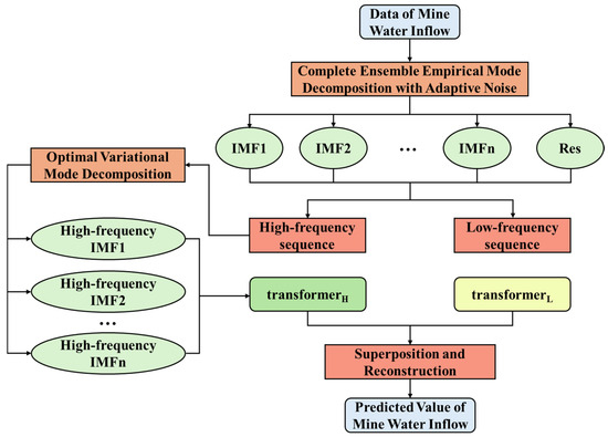
Figure 4.
CEEMDAN-OVMD-Transform modeling framework.
3. Data Processing and Model Evaluation Metrics
3.1. Data Temporalization
To ensure that each IMF component derived from CEEMDAN-OVMD decomposition complies with the training requirements of the Transformer model, it must be converted into a time-series format with the structure “time steps × input dimensions.” This process employs a sliding window mechanism to establish correlations between current and past data, providing temporal support for future water inflow predictions. For example, with a sliding window step size of s = 5, the time step length is set to 5. Sequences of IMF components for periods such as “Day 1–5,” “Day 2–6,” and so on are sequentially extracted as input samples for the model. The corresponding output samples serve as target values for water inflow predictions on “Day 6,” “Day 7,” and subsequent days. The data reconstruction rules are detailed in Table 1.

Table 1.
Data reconstruction results.
3.2. Evaluation Indicators
To evaluate the effectiveness of the proposed prediction method, this paper selects four evaluation metrics commonly used in regression problems: mean absolute error, root mean square error, mean absolute percentage error, and the goodness-of-fit coefficient of determination, R2. The formulas for each of these evaluation metrics are provided, respectively.
where and are the true and predicted values of a given sample, respectively; N is the number of samples; and are the mean of the true values and the mean of the predicted values, respectively.
4. Mine Water Inflow Prediction Study Results
4.1. Overview of the Study Area
Heidaigou Coal Mine is located in Xuejiawan Town, the government seat of Jungar Banner in Inner Mongolia Autonomous Region, with a mine area of 3.3960 km2 and a design production capacity of 900,000 t/a. The mine has four main mineable coal seams, which are the No. 4 and No. 5 seams and the Shanxi Formation, namely, No. 6 and No. 9 seams stored in the Taiyuan Formation, and No. 5 and No. 6 seams are mainly mined at present. The main aquifers in the mine are a loose rock pore-diving aquifer, a clastic rock pore and fissure pressurized aquifer, and a gray rock karst pressurized water aquifer.
As shown in Figure 5, Heidaigou coal mine water inflow composition is mainly 6 coal seam water inflow, accounting for 90%, 5 coal seam water inflow accounted for 10%; mainly 6 coal seam top and bottom plate sandstone fissure water and water in the mining airspace, 5 coal seam is mainly for the top plate sandstone fissure water and water in the mining airspace. The main water discharge points of the mine are the main alley, the working face trough, the mining hollow area, and the roof slab water discharge drilling holes. The mine water outflow from the main roadway is mainly in the form of dripping and drenching from the roadway roof and side walls.
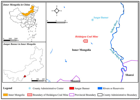
Figure 5.
Geographical location of the study area.
4.2. Characteristics and Preprocessing of Water Inflow Data
This study collected mine water inflow data from the Heidaigou Coal Mine between 1 January 2024 and 30 November 2024, comprising 334 daily records of unit water inflow. As shown in Figure 6, the maximum water inflow at Heidaigou Coal Mine was 67.0 m3/h, while the minimum was 40.3 m3/h. For modeling and validation purposes, 80% of the data (from 1 January 2024 to 22 September 2024) was used as the training set, and the remaining 20% (from 23 September 2024 to 30 November 2024) served as the test set.
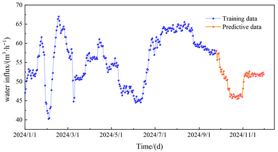
Figure 6.
Mine water inflow data.
4.3. Decomposition of Mine Water Inflow Data
As shown in Figure 6, the mine water inflow data at Heidaigou Mine shows significant fluctuations and low stationarity, with a maximum of 67.0 m3/h and a minimum of 40.3 m3/h. To improve the model’s ability to learn the variation patterns of water inflow data, the dataset was preprocessed using CEEMDAN. For this CEEMDAN process, the number of noise additions was set to 100, and the noise weight was chosen through trial and error as 0.005. The decomposition results are shown in Figure 7. Using CEEMDAN, the mine water inflow time series was broken down into five IMFs and one Res. By denoising and decoupling the original data, CEEMDAN makes each component more stationary and organized, thus enhancing the model’s learning efficiency.
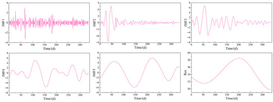
Figure 7.
CEEMDAN decomposition results.
Sample entropy is an important measure for assessing the complexity of time series data, with higher values indicating more randomness and inherent complexity. As shown in Table 2, the sample entropy value of the IMF1 component obtained through CEEMDAN decomposition reaches 1.3418, significantly higher than those of IMF2~IMF5 and Res, identifying it as a typical high-frequency fluctuation sequence. In the context of the geological and mining conditions at the Heidaigou Coal Mine, this high-frequency component corresponds to short-term, sudden water inflow triggers. These include disturbances from roadway excavation in the working face, instantaneous water inflow from temporary roof drainage boreholes, or short-duration heavy rainfall rapidly recharging the shallow loose rock pore phreatic aquifer through surface fractures, resulting in short-term, highly random fluctuations in water inflow. IMF2~IMF5 are low-frequency components, with sample entropy values ranging from 0.1372 to 0.4972, representing medium-term, stable sources of water inflow recharge within the mine. These mainly reflect continuous seepage recharge from sandstone fissure water in the coal seam roof and the slow release of accumulated water in goafs under gravity. Variations in water inflow caused by these factors show longer cycles and overall stable trends. Res represents the residual term, with the lowest sample entropy value (0.0497), indicating the long-term trend features of mine water inflow. This is primarily linked to steady long-term recharge from the limestone karst confined aquifer, combined with the cumulative effects of slowly changing formation stress and the ongoing development of roof fractures caused by long-term mining activities affecting water inflow. The high complexity of the high-frequency component IMF1 notably increases the difficulty for subsequent prediction models to learn effectively. Therefore, further decomposition is necessary to reduce its complexity, laying the foundation for models to accurately capture data patterns.
Table 2.
Sample Entropy of Each Component in CEEMDAN Decomposition.
The OVMD method was used to decompose the IMF1 component, with the penalty factor alpha set to 2000 through trial and error and the fidelity coefficient kept at the default value of 0.05. Table 3 shows the center frequencies of the decomposed components for different K values. When K = 4, similar center frequencies appeared, leading to over-decomposition. Therefore, the best number of modes was chosen as K = 3 to avoid overlapping center frequencies and prevent mode mixing. This ensures an even distribution of frequencies across components and maintains physically meaningful interpretations.
Table 3.
Center Frequencies for Different Values of K.
The decomposition results are displayed in Figure 8. As shown, the frequency distribution of each component is more uniform than in the original sequence, enabling the model to better recognize the underlying patterns in the data.
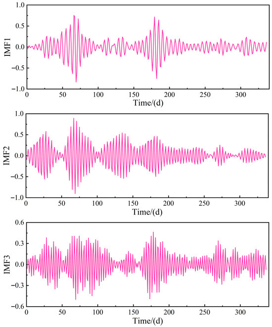
Figure 8.
OVMD decomposition results.
The synergistic decomposition of CEEMDAN and OVMD effectively improves the information features of the water inflow sequence components. CEEMDAN reduces modal aliasing with adaptive white noise, breaking down the original sequence into five IMFs and one Res, each showing distinct frequency ranges without overlapping information. When OVMD applies secondary decomposition to IMF1, it further isolates high-frequency sub-components, creating significant frequency differences between the high- and low-frequency parts after this step. This process reduces redundancy and collinearity, enabling the Transformer to better learn the water inflow driving patterns of each component, which decreases overfitting risks and lowers computational demands.
4.4. Forecast Results and Analysis
To enable data processing for Transformer training, each IMF component undergoes temporal sequence reconstruction. After multiple training trials, it was determined that a sliding step size of s = 4 yields optimal model performance. Consequently, all IMF sequences are segmented with a step size of 4. The Transformer architecture used in this training consists of 2 encoder layers, followed by 1 pooling layer and 1 fully connected layer. Key hyperparameters are set as follows: 8 multi-head attention heads, 64 units in the fully connected network, a dropout rate of 0.5, a batch size of 64, and 200 training epochs. The Transformer model predicts time-series data for each IMF component separately, and the final mine water inflow prediction is obtained by summing the forecasted results of all components.
To thoroughly evaluate the predictive performance of the proposed method, construct CEEMDAN-OVMD-BP, CEEMDAN-OVMD-SVM, CEEMDAN-OVMD-GRU, CEEMDAN-OVMD-LSTM, and Transformer models, respectively, for comparative experimental results. The comparative results are shown in Figure 9 and Figure 10, which display the mine water inflow prediction comparisons and linear fitting results across all methods.
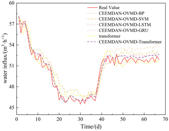
Figure 9.
Comparison of mine water inflow predictions for each model mine.
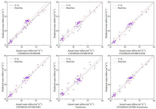
Figure 10.
Comparison of linear fitting of mine water inflow prediction results.
As shown in Figure 9, CEEMDAN-OVMD-BP and CEEMDAN-OVMD-SVM exhibit notable deviations in prediction results when data trends shift. The surface BP and SVM algorithms struggle to effectively learn the characteristics of various components in the mine water inflow data, resulting in poor prediction performance. Meanwhile, the single Transformer fails to fully capture the hidden information in the data, leading to predictions that lag. In contrast, CEEMDAN-OVMD-GRU, CEEMDAN-OVMD-LSTM, and CEEMDAN-OVMD-Transformer perform better in fitting the data and show no lag, especially during large data changes, demonstrating strong tracking ability. As shown in Figure 10, the linear fit comparison of the prediction results indicates that CEEMDAN-OVMD-GRU, CEEMDAN-OVMD-LSTM, and CEEMDAN-OVMD-Transformer produce predicted data points that are more evenly distributed and closely clustered around the Y = X line. The fitted line closely matches the Y = X line, resulting in smaller surface prediction errors. Conversely, the fitting lines and data distributions of the other three models significantly deviate from the Y = X line. Based on this analysis, decomposing the original data using CEEMDAN and OVMD methods can reveal periodic patterns at different temporal frequencies, reduce noise in the water inflow data series, and extract essential information from the raw sequence. As a result, LSTM, GRU, and Transformer models all demonstrate strong performance in time-series forecasting.
To evaluate each model’s prediction accuracy, MAE, RMSE, MAPE, and R2 were used for further assessment. The results are displayed in Table 4. Comparison shows that the CEEMDAN-OVMD-Transformer model performed best across all metrics:
Table 4.
Comparison of evaluation indicators of different methods.
Its MAE of 0.507 indicates an approximately 34.50% reduction compared to the standalone Transformer model, reflecting minimal average absolute deviation between predicted and actual water inflow values. This model predicts daily water inflow fluctuations more precisely.
With an RMSE of 0.613, lower than both CEEMDAN-OVMD-GRU and CEEMDAN-OVMD-SVM, the model has a smaller mean squared error. When handling extreme data points like peaks or troughs, its fluctuation amplitude is significantly less than in other models, demonstrating higher stability.
The MAPE of 0.010 is similar to CEEMDAN-OVMD-LSTM and CEEMDAN-OVMD-GRU, but much lower than CEEMDAN-OVMD-BP and the standalone Transformer. This indicates that the model’s relative error remains within 1%, showing less deviation in tracking water inflow trend changes.
5. Discussion
In mine water inflow prediction, combining modal decomposition and deep learning is a key approach. Hou et al.’s [17] CEEMDAN-BO-BiGRU, Wang et al.’s [15] VMD-BiLSTM, Bian et al.’s [20] CEEMDAN-NGO-LSTM, and Qin et al.’s [21] CNN-LSTM all use single-modal decomposition to reduce data complexity and improve prediction accuracy. However, these studies did not perform secondary purification on high-frequency sequences, making them vulnerable to deviations caused by high-frequency noise during sudden water inflow events. This study employs a dual-modal decomposition method, CEEMDAN-OVMD, which initially breaks down the original sequence into five IMFs and one Res, then further decomposes high-frequency IMFs to achieve a more balanced frequency distribution in high-frequency subcomponents, thus further minimizing prediction errors.
Regarding model architecture, the Transformer model is less commonly used in mine water inflow prediction. In other fields, Hu et al. [22] used it for landslide prediction, achieving an R2 of 0.9442, while Yang et al. [23] introduced a PCA-Transformer model for gas concentration prediction, reaching an MAE of 0.0203. These results demonstrate its advantages in capturing long-term temporal dependencies and adapting to non-stationary data. This study applies the Transformer to handle multi-frequency components, automatically assigning long-term trend weights to low-frequency IMFs and enhancing short-term correlations for high-frequency subcomponents, outperforming traditional recurrent neural networks.
This study has several limitations, mainly in three areas: First, the research data were collected from the Heidaigou Coal Mine, which has a relatively small sample size, limiting the ability to fully utilize the advantages of the Transformer model for large-scale data. Second, some key model parameters were chosen through trial-and-error and empirical methods, which may not have achieved the optimal global configuration, thereby somewhat restricting the model’s overall performance. Third, the study focused only on historical water inflow time-series data and did not include external factors such as geological structures, weather conditions, and mining activities, making it difficult to fully understand the complex drivers of water inflow.
Regarding the issues mentioned above, future research could follow three steps: First, gather data from various coal mines with different hydrological and geological conditions and increase the sample size for each mine. This will enhance the model’s ability to generalize by including more diverse and extensive data. Second, use advanced optimization algorithms to calibrate model parameters globally instead of relying on trial and error, enabling the model to reach its full predictive potential. Finally, create a multi-factor input system that incorporates external influences such as geological, weather, and mining conditions, shifting from a simple time-series approach to a multi-dimensional coupled prediction. This will improve both the scientific accuracy and practical usefulness of the forecasts.
6. Conclusions
This study focuses on the mine water inflow data from the Heidaigou Coal Mine and constructs a CEEMDAN-OVMD-Transformer hybrid prediction model to predict changes in mine water inflow. The model’s performance is compared with CEEMDAN-OVMD-BP, CEEMDAN-OVMD-SVM, CEEMDAN-OVMD-LSTM, CEEMDAN-OVMD-GRU, and Transformer models. The main conclusions are as follows:
- (1)
- By combining CEEMDAN-OVMD decomposition, the original sequence is broken into IMFs with different frequencies and amplitudes, enabling multi-scale separation of mine water inflow data. This converts chaotic mixed data into organized subsequences, helping the Transformer model learn the underlying patterns of water inflow dynamics.
- (2)
- High-frequency IMFs obtained from CEEMDAN undergo secondary decomposition through OVMD to refine the high-frequency signals. This purification decreases the difficulty for the Transformer to process high-frequency components, allowing it to focus on learning true patterns. As a result, the accuracy of water inflow predictions improves.
- (3)
- Through model comparison, the CEEMDAN-OVMD-Transformer model proposed in this paper employs the CEEMDAN primary decomposition and OVMD secondary refinement within a dual-modal framework to extract complex features from water inflow sequences. By integrating the Transformer to capture long-term temporal dependencies, it thoroughly explores and learns the hidden variation patterns in historical mine water inflow data, leading to improved predictive accuracy for mine water inflow. This method can be applied to short-term water inflow forecasting in similar mines, providing a foundation for mine water prevention and control.
Author Contributions
Writing—original draft preparation, Y.L.; writing—review and editing, Q.W.; data curation, F.L. All authors have read and agreed to the published version of the manuscript.
Funding
This research was funded by National Key Research and Development Program of China, grant number 2023YFC3012100.
Institutional Review Board Statement
Not applicable.
Informed Consent Statement
Not applicable.
Data Availability Statement
If interested in the data used in the research work, contact liyang@cctegxian.com for the original dataset.
Conflicts of Interest
Author Yang Li was employed by the company CCTEG Xi’an Research Institute (Group) Co., Ltd. The remaining authors declare that the research was conducted in the absence of any commercial or financial relationships that could be construed as a potential conflict of interest.
References
- Hou, E.; Xu, L.; Rong, T. Time series prediction of mine water inflow from Binchang Dafosi mine. J. Xi’an Univ. Sci. Technol. 2024, 44, 490–500. [Google Scholar]
- Yang, J.; Pu, R. Research on the distribution characteristics and water filling modes of mine water inflow in western mining areas of China. Coal Sci. Technol. 2025, 1–13. [Google Scholar]
- Yingying, D.; Shangxian, Y.; Huiqing, L.; Wei, L.; Qixing, L.; Rongrong, Q.; Changsen, B.; Xiangxue, X.; Shuqian, L. Prediction of mine water inflow along mining faces using the SSA-CG-Attention multifactor model. Coal Geol. Explor. 2024, 52, 111–119. [Google Scholar]
- Liu, H.; Liu, G.; Ning, D.; Fan, J.; Chen, W. Mine water inrush prediction method based on VMD-DBN model. Coal Geol. Explor. 2023, 51, 13–21. [Google Scholar]
- Zhang, Z.; Li, W. Comparative Study on Prediction Methods of Mine Inflow: A Case Study of Dazhuang Coal Mine in Gansu Province. Northwestern Geol. 2022, 55, 355–360. [Google Scholar]
- Zhou, Q.; Wang, D.; Dang, Z.; Huo, C.; Su, J.; Liu, C.; Gu, L.; Li, J. Research and comparative analysis of mine water inflow prediction method: A case study of Donggou Coal Mine in Xinjiang. Coal Sci. Technol. 2024, 52 (Suppl. S1), 211–220. [Google Scholar]
- Zhao, Y.; Li, X. Bi-RNN and GMS coupled prediction of water inflow in metal open-pit mines. Coal Geol. Explor. 2024, 52, 155–169. [Google Scholar]
- Li, J.; Gao, P.; Wang, X.; Zhao, S. Prediction of mine water inflow based on Chaos—Generalized Regression Neural Network. Coal Sci. Technol. 2022, 50, 149–155. [Google Scholar]
- Meng, X.; Shi, H. A Survey of Transformer-based Model for Time Series Forecasting. J. Front. Comput. Sci. Technol. 2025, 19, 45–64. [Google Scholar]
- Liang, H.; Liu, S.; Du, J. Review of Deep Learning Applied to Time Series Prediction. J. Front. Comput. Sci. Technol. 2023, 17, 1285–1300. [Google Scholar]
- Liu, X.; Ji, Y.; Zhu, K.; Zhao, C.; Li, K.; Li, C.; Yuan, C.; Li, P.; Yan, P. Construction and application of a TCN-LSTM-SVM-based time series prediction model for water inflow in coal seam roofs. Coal Geol. Explor. 2025, 53, 201–211. [Google Scholar]
- Thirunavukarasu, A.J.; Ting, D.S.J.; Elangovan, K.; Gutierrez, L.; Tan, T.F.; Ting, D.S.W. Large language models in medicine. Nat. Med. 2023, 29, 1930–1940. [Google Scholar] [CrossRef] [PubMed]
- Annan, R.; Qingge, L. Artificial intelligence in COVID-19 research: A comprehensive survey of innovations, challenges, and future directions. Comput. Sci. Rev. 2025, 57, 100751. [Google Scholar] [CrossRef]
- Zhou, G.; Qu, Z.; Zhan, Z. Fusion of wavelet denoising and VMD-NTEO for transmission line fault localization. Proc. CSU-EPSA 2025, 37, 141–150. [Google Scholar]
- Wang, F.; Rong, T.; Hou, E.; Fan, Z.; Tan, E. VMD-BiLSTM Combined Model-based Mine Research on time series prediction method of water influx. Min. Res. Dev. 2024, 44, 143–151. [Google Scholar]
- Qi, X.; Shao, L.; Xing, Y. ARMA prediction model of mine water inflow based on EMD. J. Liaoning Tech. Univ. (Nat. Sci.) 2020, 39, 509–513. [Google Scholar]
- Hou, E.; Xia, B.; Wu, Z.; Rong, T. Mine Water Inflow Prediction Based on CEEMDAN-BO-BiGRU. Sci. Technol. Eng. 2023, 23, 12012–12019. [Google Scholar]
- Torres, M.E.; Colominas, M.A.; Schlotthauer, G.; Flandrin, P. A complete ensemble empirical mode decomposition with adaptive noise. In Proceedings of the IEEE International Conference on Acoustics, Speech Signal Processing, Prague, Czech Republic, 22–27 May 2011; pp. 4144–4147. [Google Scholar]
- Vaswani, A.; Shazeer, N.; Parmar, N.; Uszkoreit, J.; Jones, L.; Gomez, A.N.; Kaiser, Ł.; Polosukhin, I. Attention Is All You Need. In Proceedings of the Advances in Neural Information Processing Systems, Long Beach, CA, USA, 4–9 December 2017; pp. 3778–3786. [Google Scholar]
- Bian, J.; Hou, T.; Ren, D.; Lin, C.; Qiao, X.; Ma, X.; Ma, J.; Wang, Y.; Wang, J.; Liang, X. Predicting mine water inflow volumes using a decomposition-optimization algorithm-machine learning approach. Sci. Rep. 2024, 14, 17777. [Google Scholar] [CrossRef] [PubMed]
- Qin, J.; Xu, S.; Zhang, B.; Zong, J.; Zhang, J. Research on Prediction Method of Mine Water Inflow Based on CNN-LSTM Model. Coal Technol. 2025, 44, 234–239. [Google Scholar]
- Hu, X.; Li, B.; Shi, Y.; Yin, J.; Li, C.; Yu, Z. NRBO dual-optimized VMD-Transformer model landslide prediction method. Bull. Surv. Mapp. 2025, 1, 143–150. [Google Scholar]
- Yang, J.; Shu, L.; Zhang, S.; Quin, K.; Cui, C. Research on a PCA-transformer-based prediction algorithm for gas concentration in working face. J. Mine Autom. 2025, 51, 1–7. [Google Scholar]
Disclaimer/Publisher’s Note: The statements, opinions and data contained in all publications are solely those of the individual author(s) and contributor(s) and not of MDPI and/or the editor(s). MDPI and/or the editor(s) disclaim responsibility for any injury to people or property resulting from any ideas, methods, instructions or products referred to in the content. |
© 2025 by the authors. Licensee MDPI, Basel, Switzerland. This article is an open access article distributed under the terms and conditions of the Creative Commons Attribution (CC BY) license (https://creativecommons.org/licenses/by/4.0/).