Article

A Data-Driven Framework for Modeling Car-Following Behavior Using Conditional Transfer Entropy and Dynamic Mode Decomposition

by
Poorendra Ramlall
and
Subhradeep Roy
*,†
Mechanical Engineering Department, Embry-Riddle Aeronautical University, Daytona Beach Campus, 1 Aerospace Blvd, Daytona Beach, FL 32114, USA
*
Author to whom correspondence should be addressed.
These authors contributed equally to this work.
Appl. Sci. 2025, 15(17), 9700; https://doi.org/10.3390/app15179700
Submission received: 11 July 2025 / Revised: 27 August 2025 / Accepted: 28 August 2025 / Published: 3 September 2025
(This article belongs to the Section Transportation and Future Mobility)

Abstract

Accurate modeling of car-following behavior is essential for understanding traffic dynamics and enabling predictive control in intelligent transportation systems. This study presents a novel data-driven framework that combines information-theoretic input selection via conditional transfer entropy (CTE) with dynamic mode decomposition with control (DMDc) for identifying and forecasting car-following dynamics. In the first step, CTE is employed to identify the specific vehicles that exert directional influence on a given subject vehicle, thereby systematically determining the relevant control inputs for modeling its behavior. In the second step, DMDc is applied to estimate and predict the dynamics by reconstructing the closed-form expression of the dynamical system governing the subject vehicle’s motion. Unlike conventional machine learning models that typically seek a single generalized representation across all drivers, our framework develops individualized models that explicitly preserve driver heterogeneity. Using both synthetic data from multiple traffic models and real-world naturalistic driving datasets, we demonstrate that DMDc accurately captures nonlinear vehicle interactions and achieves high-fidelity short-term predictions. Analysis of the estimated system matrices reveals that DMDc naturally approximates kinematic relationships, further reinforcing its interpretability. Importantly, this is the first study to apply DMDc to model and predict car-following behavior using real-world driving data. The proposed framework offers a computationally efficient and interpretable tool for traffic behavior analysis, with potential applications in adaptive traffic control, autonomous vehicle planning, and human-driver modeling.

1. Introduction

Modeling and understanding traffic dynamics remains a fundamental challenge in transportation science, with far-reaching implications for roadway design, congestion management, autonomous vehicle control, and the development of smart mobility systems [1,2]. As transportation networks grow more complex due to urbanization, increasing vehicle density, and the emergence of connected and autonomous vehicles, the demand for accurate, interpretable, and adaptable traffic models becomes increasingly critical. Central to this effort is the ability to understand and predict individual driver behavior, which is essential for enhancing traffic safety, improving operational efficiency, and ensuring effective coordination between human and automated driving agents. At the microscopic scale, car-following behavior, which describes how drivers adjust their speed and acceleration based on the actions of neighboring vehicles, serves as a foundational mechanism in traffic flow modeling. This elementary interaction gives rise to a range of emergent traffic phenomena, including shockwaves, stop-and-go waves, and capacity drops [3,4], making it a critical focus for both theoretical and applied transportation research. Car-following models provide the microscopic foundation for simulating and analyzing these interactions. Notable examples include the Optimal Velocity Model [5], where a driver’s acceleration is guided by a desired speed that depends on headway. The Intelligent Driver Model [6] introduces more realistic driving behaviors, including braking intensity and relative speed. The Backward-Looking Motion Information model [7] advances previous frameworks by accounting for the influence of both leading and following vehicles—an essential refinement for accurately capturing the dynamics of traffic flow [8]. While these models help reproduce general traffic patterns, their underlying assumptions often overlook the variability and complexity of real-world driving. As a result, they struggle to account for individual differences in driver behavior and the heterogeneity present in actual traffic scenarios [9].
To address this gap, researchers have increasingly turned to real-world traffic datasets [10,11,12], which allow for the empirical analysis of driver behavior and interaction dynamics. These datasets offer a rich foundation for both validating existing models and enabling the development of more advanced modeling approaches. However, analyzing such data requires robust methodologies capable of uncovering the structure of the underlying dynamics without relying on oversimplified assumptions. Data-driven modeling frameworks provide a promising path forward in this regard. In particular, machine learning techniques have been applied to extract model parameters or directly learn behavioral rules from empirical observations [13,14]. While powerful, these black-box models often suffer from limited interpretability and poor generalizability, raising concerns about transparency and trustworthiness [15]. For instance, Xiong et al. [1] use machine learning-based parameter estimation for IDM calibration, but the learned dynamics remain difficult to interrogate and understand from a systems-theoretic perspective.
Alternative approaches leverage recent advances in data-driven system identification rooted in dynamical systems theory [16,17,18,19,20]. Reduced-order modeling enables the representation of high-dimensional traffic data using a simplified model that captures the most significant dynamics. This improves interpretability, reduces the risk of overfitting, and allows efficient learning from smaller datasets [21,22]. One such method, dynamic mode decomposition (DMD) [23,24], offers a principled framework for approximating the evolution of complex nonlinear systems using linear models. DMD has gained traction in diverse fields, including fluid mechanics, neuroscience, and robotics, due to its simplicity, computational efficiency, and capacity to extract dominant modes of behavior from high-dimensional data [25,26]. A powerful extension, dynamic mode decomposition with control (DMDc), incorporates exogenous inputs into the framework [27], enabling the joint estimation of system dynamics and external influences. DMDc has shown promise in applications ranging from epidemiology [28], biology [29], swarm modeling [30], and neural diagnostics [31] to aircraft control [32] and transportation modeling [2,33].
In addition to system identification techniques, information-theoretic tools such as transfer entropy provide a powerful method for uncovering directional relationships between interacting vehicles [34,35,36]. Unlike correlation-based measures, transfer entropy captures nonlinear dependencies and distinguishes cause from effect in temporal processes. These metrics have been successfully applied to a wide range of complex systems, including human brain activity [37], animal collective behavior [38,39,40], policy-making [41,42], and financial markets [43]. In the context of traffic, it enables the quantification of how one vehicle’s behavior influences another, revealing latent structures of driver interaction that are not readily observable. Incorporating this framework into the modeling process supports the principled selection of model variables.
Motivated by these developments, this study introduces a novel data-driven framework for analyzing car-following dynamics using transfer entropy and DMDc. We first employ conditional transfer entropy to uncover latent influence structures between vehicles, thereby enabling principled selection of state and control input variables for system identification. We then apply DMDc to both simulated and real-world datasets to estimate and predict vehicle trajectories. Through extensive validation, including error quantification, system matrix inspection, and prediction analysis, we demonstrate that this approach yields accurate, interpretable, and computationally efficient models of car-following behavior. This work represents the first use of DMDc for microscopic traffic modeling and forecasting, offering new avenues for data-informed traffic analysis and control.

2. Methods

In this study, we employ a data-driven framework for traffic modeling that integrates information theory and DMDc to perform both system identification and prediction. We begin by evaluating the framework using synthetic data generated from two car-following models, allowing us to assess its effectiveness when the ground truth is known. We then extend the analysis to real-world car-following traffic data. The accuracy of both inferred system dynamics and predictive performance is evaluated using multiple performance metrics. Section 2.1 outlines the underlying mechanics of the longitudinal traffic models and details the simulation parameters used to generate the synthetic data. Section 2.2 describes the structure and characteristics of the real-world traffic data. Section 2.3 presents the information theory-based component of our data-driven framework, which is used to identify the state variables that govern traffic interactions. These selected variables then serve as input to the DMDc-based formulation described in Section 2.4, which constructs a dynamical model to estimate and predict traffic behavior. Finally, Section 2.5 defines the metrics used to evaluate model performance. Figure 1 presents a schematic overview of the proposed framework. All modeling, data processing, and analysis are conducted using MATLAB R2024a.

2.1. Traffic Models

In this study, two longitudinal traffic models are used to generate synthetic data. Longitudinal traffic models describe how a driver controls acceleration and deceleration in response to the movement of surrounding vehicles along a single lane. Within this class, car-following models are a widely used subset that assume that each vehicle responds primarily to its immediate front car. Prominent examples of such models include the Intelligent Driver Model (IDM) and the Optimal Velocity Model (OVM). These models provide a foundational basis for extensions that incorporate additional driving behaviors, such as augmenting the traditional IDM framework with lane-changing dynamics [44].
The two models used in this study are the Backward-Looking Motion Information model [7] and a hybrid traffic model that combines the alternating dynamics of both OVM and IDM.

2.1.1. Backward-Looking Effect and Motion Information (BLMI) Model

The BLMI model extends traditional car-following models by incorporating not only information from multiple preceding vehicles but also influence from rear vehicles [7]. In contrast, conventional car-following models typically assume that a vehicle responds solely to its immediate lead vehicle. In the BLMI model, the acceleration of the n-th vehicle is defined as follows:
d v n d t = σ BLMI p m l = 1 m V F ( Δ x n + l 1 ) + ( 1 p ) V B ( Δ x n 1 ) v n + λ 1 m l = 1 m v n + l v n
Here, v n is the velocity of the n-th vehicle, σ BLMI is a parameter representing the sensitivity of the driver, and m denotes the number of vehicles ahead from which the subject vehicle draws information. The parameter λ captures the influence of the velocity difference between the subject vehicle and the average velocity of the m vehicles in front. The distance headway Δ x n = x n + 1 x n represents the spacing between a vehicle and its immediate leader. The forward and backward velocity functions, V F and V B , are defined below. The parameter p [ 0 , 1 ] controls the relative influence of front and rear vehicles. When p = 1 and m = 1 , only front vehicle information is considered, replicating the traditional car-following assumption. For 0 < p < 1 , both front and rear vehicles contribute to the model, with rear influence becoming increasingly dominant as p decreases below 0.5. The forward and backward velocity functions are given by
V F ( Δ x n ) = v max F 2 tanh ( Δ x n h c ) + tanh ( h c ) V B ( Δ x n 1 ) = v max B 2 tanh ( h c Δ x n 1 ) + tanh ( h c )
Here, v max F and v max B denote the maximum desired speeds based on front and rear vehicle interactions, respectively, while h c represents the desired safe spacing between vehicles.
Simulations using the BLMI model are conducted under periodic boundary conditions, representing vehicles traveling on a circular ring using the parameters outlined in Table 1a. The vehicles are initially uniformly positioned along the track, with initial velocities based on the forward and backward optimal velocity functions as follows:
x 1 ( 0 ) = L / N + 1 x n ( 0 ) = n N L , n = 2 , 3 , 4 , , N x ˙ n ( 0 ) = p V F ( L / N ) + ( 1 p ) V B ( L / N )
The position and velocity of the vehicles are updated as follows:
x n ( t + Δ t ) = x n ( t ) + v n ( t ) Δ t + 1 2 a n ( t ) Δ t 2 v n ( t + Δ t ) = v n ( t ) + a n ( t ) Δ t
where a n ( t ) is as defined by Equation (1).

2.1.2. Hybrid Traffic Model

To evaluate the performance of our proposed data-driven framework under more realistic and time-varying conditions, we construct a hybrid traffic model that captures dynamic shifts in driver behavior. This approach is based on the understanding that human drivers may not consistently follow a single car-following strategy but instead switch between different behavioral modes over time. In this setup, vehicles alternate between the OVM and the IDM across five time intervals of equal duration. The simulation begins with OVM dynamics, such that vehicles follow OVM-based acceleration rules in the first, third, and fifth intervals and IDM-based rules in the second and fourth intervals. This hybrid configuration allows us to assess the robustness of the data-driven framework in capturing transitions across different governing dynamics.
Similar to the BLMI model, the hybrid model is used to generate synthetic data by simulating vehicles on a circular ring with periodic boundary conditions. Following the setup in [45], the vehicle length and desired speed for IDM are set to l v = 5 and v 0 = 30 km / h , respectively. All other IDM parameters follow the standard values reported in [6]. For the OVM, parameters are selected based on empirical findings from [46]. Similar to the BLMI setup, vehicles are uniformly distributed along the ring at initialization and assigned initial velocities randomly sampled from a uniform distribution in the range [0, 1]. Simulations are run for T sim = 2500 s with a time step of d t = 0.01 s, using the OVM and IDM parameters summarized in Table 1b.
To shed light on the operating principles of the OVM and IDM models, we briefly describe how each defines vehicle acceleration based on the influence of the immediate front vehicle, typically as a function of relative speed and spacing.
  • Optimal Velocity Model (OVM)
The OVM is a car-following model that defines the acceleration of each vehicle based on the difference between its current velocity and a desired or ‘optimal’ velocity V ( s ) , which depends on the spacing s to the vehicle directly ahead. The acceleration is expressed as
d v d t = σ OVM V ( s ) d x d t
where σ OVM is a sensitivity parameter capturing driver responsiveness and vehicle dynamics [5], and V ( s ) is the optimal velocity function, defined as
V ( s ) = α tanh β ( s s 0 ) + v 0
In this expression, s 0 represents the minimum safe following distance, and the parameters α , β , and v 0 control the shape, steepness, and offset of the velocity response, respectively.
The use of the hyperbolic tangent function ensures a smooth transition in the desired speed based on spacing: when the spacing s is significantly larger than s 0 , the argument of the tanh function becomes large, and V ( s ) asymptotically approaches α + v 0 . This implies that vehicles tend to maintain their maximum desired speed when the gap is sufficiently large. Conversely, as the spacing decreases toward s 0 , the optimal velocity is reduced, prompting the vehicle to slow down, thereby ensuring safe car-following behavior.
  • Intelligent Driver Model (IDM)
The IDM is another widely used car-following model that determines a vehicle’s acceleration based on its current speed, the relative speed to the leading vehicle, and the spacing. The acceleration is given by
d v d t = a max 1 v v 0 δ s v , Δ v s 2
where a max is the maximum acceleration, v 0 is the desired velocity, and δ is the acceleration exponent, typically set to δ = 4 [6]. The variable Δ v denotes the relative velocity between the subject and leading vehicles, s is the current spacing, and s is the desired spacing, defined as
s = s 0 + max 0 , v Δ T + v Δ v 2 a max b
Here, s 0 is the minimum allowable spacing, Δ T is the desired time gap (temporal headway), and b is the comfortable deceleration rate [6]. The IDM formulation in Equation (6) includes two main components. The first term governs acceleration, which decreases to zero as the vehicle approaches the desired speed v 0 . The second term accounts for braking behavior by increasing deceleration as the spacing decreases. The deceleration aggressiveness is modulated by the parameter b. Equation (6) is solved using the ballistic method [47] to determine the vehicles’ speed and position. Special consideration is applied in scenarios where the leading vehicle is stationary, which may result in negative velocities or unrealistic backward motion. To prevent this, conditional constraints are imposed, and the vehicle’s state is updated as follows:
v t + Δ t = { 0       v ( t ) + d v d t Δ t < 0 v ( t ) + d v d t Δ t       otherwise                                           x t + Δ t = { x ( t ) 1 2 v 2 ( t ) d v d t 1       v ( t ) + d v d t Δ t < 0 x ( t ) + v ( t ) Δ t + 1 2 d v d t Δ t 2       otherwise
The simulation parameters for the BLMI and hybrid car-following models are provided in Table 1. The parameters used for the BLMI model are given in Table 1, part a, while the simulation parameters for the OVM and IDM components of the hybrid model are given in Table 1, part b. In each model, these parameters are selected to be in conjunction with the studies in [5,6,16,17,47] to ensure stability.

2.2. Description of Observational Data

The observational data used in this study are adopted from the benchmark dataset provided by Chen et al. in [11], which was specifically developed for car-following modeling. This comprehensive dataset includes 82,228 car-following events, curated from five publicly available driving datasets, all selected using consistent criteria.
In their work, Chen et al. compare car-following behaviors across these five data sources using a range of evaluation metrics. The five datasets include HighD [48], the Next Generation Simulation (NGSIM) dataset for highway I-80 [49], the Safety Pilot Model Deployment (SPMD) dataset [50], and data from Waymo [51] and Lyft [52]. Notably, the Waymo and Lyft datasets include mixed traffic conditions, adding further diversity to the benchmark [11]. The HighD dataset provides car-following events of 15 s duration, while a variant called HighD30 contains events lasting 30 s. The remaining datasets include events of variable lengths, with a minimum duration of 20 s [11]. The SPMD data are available in two formats, labeled ‘DAS1’ and ‘DAS2’, depending on the data acquisition system used. Each car-following event in this dataset includes four recorded variables: the spacing between vehicles, the velocity of the subject vehicle, the velocity of the leading vehicle, and their relative velocity.

2.3. Control Input Identification via Transfer Entropy

Information theory provides a principled framework for quantifying the uncertainty and information content in time-series data, making it particularly useful for analyzing interactions in complex dynamical systems [53,54,55,56]. Transfer entropy (TE) and its extension, conditional transfer entropy (CTE), are model-free information-theoretic measures designed to detect and quantify directional, potentially non-linear dependencies between processes [34,36]. Rooted in Shannon’s concept of entropy, TE measures the amount of information that the past states of a source process contribute to estimating the future states of a target process, beyond what is already explained by the target’s own past [34,35]. In essence, TE captures the average reduction in uncertainty of the target’s future when the source’s past is taken into account, thereby characterizing the direction and magnitude of information flow between interacting components [57]. CTE extends the concept of TE by quantifying the directed flow of information between two time series while conditioning on additional variables. By accounting for the influence of other potential sources, CTE isolates direct causal relationships and reduces confounding from indirect or shared influences, making it particularly effective for analyzing complex multivariate systems [17,34,36].
Consider two source processes, Y and Z, and a target process X. TE from Y to X quantifies the information flow from the source Y to the target X by comparing the predictability of X’s future based on its own past with its past augmented with the past of Y. The TE is mathematically defined as
T Y X = log p x k + 1 | x k , y k p x k + 1 | x k ,
where · denotes the average over all samples, k is the time index, and p x k + 1 | x k is the conditional probability of x k + 1 given its immediate past x k .
To account for potential confounding influences from an additional source process Z, CTE is used. It measures the directed influence from Y to X while conditioning on Z, effectively isolating direct dependencies. The CTE is defined as
C Y X | Z = log p x k + 1 | x k , z k , y k p x k + 1 | x k , z k ,
where p x k + 1 | x k , z k , y k is the conditional probability of x k + 1 given the past states of X, Y, and Z.
To compute TE and CTE, we utilize the Java Information Dynamics Toolkit for MATLAB [58], employing the Kraskov, Stögbaueand, and Grassberger estimator for non-parametric probability distribution estimation [59]. The statistical significance of the computed TE and CTE values is essential for inferring causal relationships and is evaluated using surrogate data methods that test the null hypothesis that the observed information flow is not significantly different from zero [60].
In this study, we focus exclusively on CTE, as our traffic modeling setup involves interactions among more than two time-series variables. Specifically, we define three time-series variables as observables for computing CTE. To quantify the influence of the front vehicle on the subject vehicle, we use the spacing, i.e., the gap between the subject vehicle and its immediate front vehicle, as one source variable. To capture the potential influence of the rear vehicle, we use the gap between the subject vehicle and its immediate rear vehicle as a second source variable. The third observable is the distance moved by the subject vehicle in the next time interval, which serves as the target variable in the CTE analysis. To measure the influence of the front vehicle, we define the source as the spacing, the target as the subject vehicle’s distance moved, and the condition on the distance to the rear vehicle. Conversely, to evaluate the influence of the rear vehicle, we define the source as the distance to the rear vehicle; the target, again, as the distance moved; and the condition on the forward spacing. This setup allows us to isolate the directional influence of front and rear vehicles on the subject vehicle’s motion while accounting for the potential confounding effects of the other. This CTE analysis serves as the first step in our proposed data-driven framework for discovering traffic models. Specifically, if the results indicate that only the front vehicle has a statistically significant influence on the subject vehicle’s motion, we include only the front vehicle’s states (position and velocity) as control inputs in the subsequent DMDc step. On the other hand, if significant influence is observed from both the front and rear vehicles, we would incorporate the states of both vehicles as control inputs in the DMDc modeling process. This adaptive strategy ensures that the resulting model accurately reflects the true structure of interactions captured in the data. The role of DMDc, as explained below, is then to identify the functional relationships between the selected variables and reconstruct the underlying dynamical system governing the subject vehicle’s motion.

2.4. System Identification and Prediction Using Dynamic Mode Decomposition with Control

Having identified the control inputs, in this case, the relevant interacting vehicles using CTE, we proceed to the second step of our framework: constructing a model using dynamic mode decomposition with control (DMDc). DMD is a mathematical technique originally developed to extract dominant dynamical features from fluid flows [61], and has since been extended to analyze a wide range of complex dynamical systems [23,24]. By decomposing a sequence of time-series observations into coherent spatial and temporal modes, DMD approximates the composition operator that governs the system’s evolution in time. A key advantage of DMD is that it does not rely on a predefined set of basis functions [16]; instead, it constructs data-driven modes that inherently capture the system’s behavior [23,24]. DMDc extends the standard DMD formulation by explicitly incorporating control inputs into the modeling process [27]. This extension enables the framework to not only estimate system dynamics but also predict future states in scenarios where external factors influence the evolution of the system. By separating the internal dynamics from external influences, DMDc offers a powerful data-driven approach to modeling driving behavior. In our context, the subject vehicle’s motion is modeled based on its own state and the control inputs identified through CTE, which may include the states of the front vehicle only or both front and rear vehicles.
The governing equation for the DMDc model is given by
x k + 1 = A x k + B u k ,
where x k is the state vector of the subject vehicle at time step k, u k is the control input vector composed of the influencing vehicles’ states, A is the unknown system matrix, and B is the unknown input matrix capturing how the control inputs affect the subject vehicle’s motion. DMDc is employed to estimate both the A and B matrices.
Although DMDc has been applied to various transportation-related problems, for example, vehicle dynamics and traffic flow prediction [62,63], its application to microscopic traffic modeling, such as car-following behavior, remains underexplored. In this study, we apply DMDc for the first time to both simulated and observed car-following data to estimate the governing dynamics and forecast future states. The full procedure for estimating the DMDc model using singular value decomposition is outlined in Algorithm 1.
A critical component in applying DMDc is the construction of the state–input vector, denoted as Ω , which defines both the system states to be estimated and the control inputs to be considered. To explore the effect of different observable configurations, we conduct an exploratory analysis using simulated data from both the BLMI and hybrid traffic models. Specifically, we evaluate four different formulations of Ω to assess how different combinations of state and input variables influence model estimation, as follows:
Ω 1 sim = v i Δ v i s i Ω 2 sim = v i v i + 1 x i + 1 Ω 3 sim = x i v i s i Δ v i Ω 4 sim = x i v i x i + 1 v i + 1 .
In each of the above formulations, i refers to the subject vehicle, i + 1 denotes the immediate front vehicle, x and v represent position and velocity, s i is the spacing (i.e., x i + 1 x i ), and Δ v i is the relative velocity between the subject and front vehicle. For analysis, the first vehicle in the simulated fleet is arbitrarily selected as the subject vehicle. These four choices of Ω are restricted to car-following scenarios only, consistent with the structure of the real-world dataset, which exclusively captures car-following behavior. If the CTE analysis indicates significant rear influence on the subject vehicle, the states of the rear vehicle need to be included in Ω to accurately incorporate all the relevant control inputs and model the longitudinal traffic flow.
Algorithm 1 Dynamic mode decomposition with control (DMDc).
Input: Data snapshots of system states X = { x 1 , x 2 , , x T 1 } , next-step states X =
                { x 2 , x 3 , , x T } , control inputs Y = { u 1 , u 2 , , u T 1 } , where T is the total number of
       time steps.
Output: Approximated system matrices A ˜ and B ˜ such that:
x k + 1 A ˜ x k + B ˜ u k
   
         Construct data matrices:
  1:
X x 1 x 2 x T 1
  2:
X x 2 x 3 x T
  3:
Y u 1 u 2 u T 1
       Form the augmented data input matrix:
  4:
Ω X Y                                                                  ▹ Concatenate X and Y row-wise
       Find the truncated SVD of input Ω :
  5:
Ω U ˜ Σ ˜ V ˜ , where U ˜ = U ˜ 1 U ˜ 2
       Find the truncated SVD of output X :
  6:
X U ^ Σ ^ V ^
       Reduced-order approximation of A and B :
  7:
A ˜ = U ^ X V ˜ Σ ˜ 1 U ˜ 1 U ^
  8:
B ˜ = U ^ X V ˜ Σ ˜ 1 U ˜ 2
  9:
Return  A ˜ , B ˜
For the observed traffic data, we apply DMDc to both estimate and predict the velocity dynamics of the subject vehicle. Unlike the simulated datasets, the real-world car-following data include only four recorded variables: the spacing between vehicles, the velocity of the subject vehicle, the velocity of the leading vehicle, and the relative velocity between them. As position data are not available, any state–input configuration Ω that relies on absolute position x cannot be used. Given these constraints, we define the control inputs using the relative velocity and spacing with respect to the front vehicle, resulting in the following state–input representation:
Ω obs = v i Δ v i s i
This formulation aligns with the limitations of real-world traffic sensing, where only relative kinematic information is typically accessible.
The dataset is partitioned into two subsets: a training set used to estimate the system dynamics and a testing set used to evaluate the model’s predictive accuracy by comparing predictions against ground truth using various performance metrics. A consistent train–test split is applied across all analyses, with 70% of the data allocated for training and the remaining 30% for testing.

2.5. Metrics

To evaluate the performance of the proposed framework, we employ key metrics: mean relative error (MRE), mean square error (MSE), and an additional metric, collision rate [11], computed for the analysis of the real-world data. These metrics are chosen to capture the accuracy of the estimated or predicted dynamics.
  • Mean Relative Error (MRE):
The relative absolute error quantifies the deviation between an estimated (or predicted) value z ˜ and the ground truth value z, normalized by the magnitude of the true value. It is defined as
RAE ( t ) = | z ( t ) z ˜ ( t ) | z ( t )
RAE is bounded on [ 0 , ) , with a value of zero indicating perfect estimation or prediction. As the error increases, the RAE grows monotonically, providing a scale-invariant measure of model performance. The mean relative error is defined as the time-averaged value of the relative absolute error (RAE), and is given by
MRE = 1 T t = 1 n T | z ( t ) z ˜ ( t ) | z ( t )
where T is the total number of time steps.
  • Mean Square Error (MSE):
The mean square error measures the average of the squared deviations between the estimated (or predicted) and true values, as follows:
MSE = 1 T t = 1 n T z ( t ) z ˜ ( t ) 2
Unlike MRE, which captures relative error, MSE emphasizes large deviations more strongly due to the squaring operation. A lower MSE reflects a better fit to the ground truth data in absolute terms.
  • Collision Rate:
For real-world traffic data, we also compute the collision rate, which quantifies the frequency of physically implausible events—specifically instances where the predicted spacing between the subject and front vehicle becomes negative. While the original dataset contains no collisions, negative spacing values in the predicted trajectories indicate unrealistic outcomes, suggesting a failure to preserve physical constraints. The collision rate is defined as
Collision Rate = E events N events
where E events is the number of car-following events in which s < 0 occurs at any time step, and N events is the total number of evaluated events. A lower collision rate reflects higher physical realism and improved safety consistency in the framework’s predictions.

3. Results and Discussion

We demonstrate our proposed data-driven modeling framework using two types of examples based on synthetic datasets generated from the BLMI and hybrid traffic models, as described in the Methods section. These controlled experiments serve two main purposes: first, they allow us to evaluate the reliability and robustness of the framework in modeling the traffic dynamics when the ground truth is known; second, they help us explore how different choices of state–input vectors affect model performance. Insights gained from this synthetic analysis inform the selection of input configurations and validation strategies, which are then applied to real-world traffic data to assess the framework’s effectiveness under realistic conditions.
It is important to emphasize that our proposed framework consists of two sequential steps: first, identifying the appropriate control inputs using CTE measure, and second, using DMDc to model the dynamics of the system based on these inputs. In the case of the real-world dataset, this first step is not necessary. The dataset comprises pre-identified car-following events, where it has already been established that each subject vehicle is influenced solely by its immediate front vehicle. As a result, the control input for each vehicle is limited to the front vehicle, and transfer entropy analysis is not applied in this context.
In contrast, the synthetic examples offer a more flexible and controlled environment for validating the framework. In the hybrid model, the car-following dynamics change over time, alternating between IDM and OVM formulations to reflect variability in human driving behavior. In the BLMI model, additional complexity is introduced by incorporating influence from both the front and rear vehicles. These cases enable us to rigorously test the effectiveness of the transfer entropy-based input identification step. Specifically, we examine whether transfer entropy can accurately detect the true direction and source of influence, thereby validating the framework’s ability to infer the interaction structure before proceeding to DMDc-based model estimation.

3.1. Results of Control Input Identification via Transfer Entropy

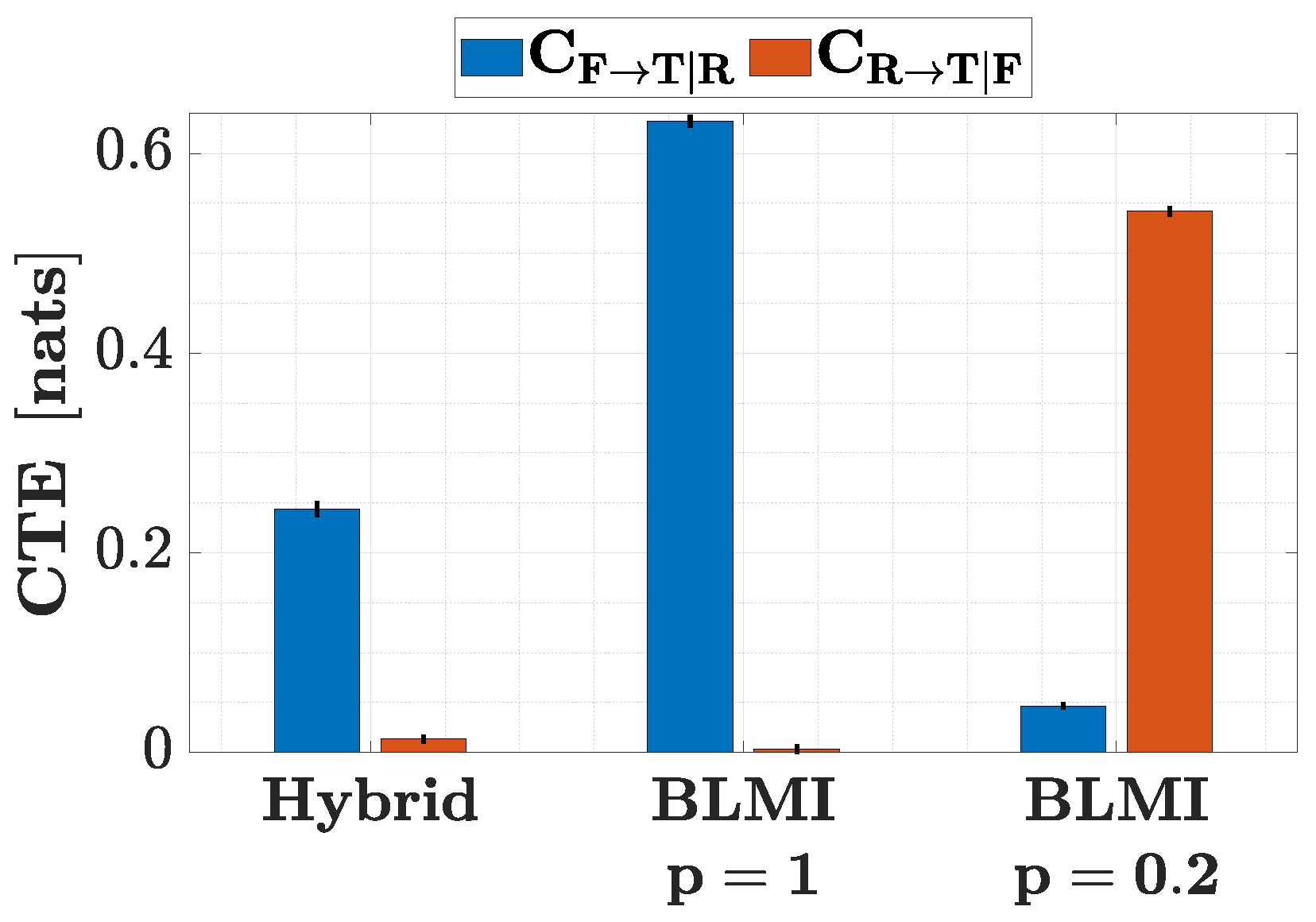
We apply CTE analysis to synthetic datasets generated from the hybrid model and the BLMI model under varying configurations of vehicle influence. For the BLMI model, we consider two cases: one with no rear influence ( p = 1 , m = 1 ), representing a pure car-following scenario where the subject vehicle is influenced only by the front vehicle, and another with dominant rear influence ( p = 0.2 m = 1 ), where the rear vehicle exerts greater influence than the front. These cases allow us to evaluate the sensitivity of CTE to directional changes in inter-vehicle interaction.
For each simulated vehicle, we compute CTE in both directions: from the front vehicle to the target conditioned on the rear ( C F T | R ) and from the rear to the target conditioned on the front ( C R T | F ). This bidirectional analysis enables us to assess whether CTE can accurately identify the dominant source of influence under different interaction dynamics. The results are presented in Figure 2, which shows the mean CTE values averaged across all simulated vehicles. Error bars denote one standard deviation, illustrating the variability in influence strength among vehicles.
As shown in Figure 2, CTE effectively captures the directional vehicle influences embedded in the synthetic models. In the hybrid model, where each vehicle follows its immediate front vehicle, CTE correctly identifies the front as the dominant source of influence, with mean values around 0.25 nats. The influence from the rear vehicle is negligible, consistent with the car-following model.
A similar pattern is observed in the BLMI model with p = 1 , which also represents a front-only influence scenario. Here, the CTE from the front vehicle is even more pronounced, exceeding 0.6 nats on average, while the rear influence remains near zero. In both cases, CTE correctly identifies the front vehicle as the sole source of influence.
When the BLMI model is configured with p = 0.2 , introducing stronger rear influence, the directionality of information flow shifts. The CTE from the rear vehicle becomes dominant, while the influence from the front decreases significantly. This outcome demonstrates CTE’s capability to detect changes in interaction structure, even in the presence of competing influences.
This ability to uncover hidden interaction dynamics using our data-driven framework highlights the practical utility of CTE as the first step in the model discovery process. By accurately identifying the dominant sources of influence, CTE provides a principled foundation for selecting relevant state and control input variables for subsequent system identification using DMDc.
For example, in the hybrid model and the BLMI model with p = 1 , where only the front vehicle influences the subject vehicle, the state–input vectors used in DMDc include the position and velocity of both the subject and front vehicles. In contrast, for the BLMI model with p = 0.2 , where influence comes from both front and rear vehicles, CTE detects this dual interaction, and the DMDc control input needs to be expanded to include the position and velocity of both the rear and the front vehicles.
In the following sections, we focus exclusively on car-following events—specifically, using the simulated dataset (hybrid model and BLMI model when p = 1 ) for model estimation and the real-world dataset for both estimation and prediction. Our focus aligns with the structure of the real-world data, which consists entirely of car-following interactions where each vehicle is assumed to be influenced only by its immediate front vehicle.

3.2. Car-Following Model Estimation Using DMDc

Having identified the relevant control inputs using conditional transfer entropy, we now apply DMDc to estimate the car-following dynamics for the simulated model scenarios. For clarity, we reiterate the previously defined sets of Ω that will be utilized in the DMDc analysis.
Ω 1 sim = v i Δ v i s i Ω 2 sim = v i v i + 1 x i + 1 Ω 3 sim = x i v i s i Δ v i Ω 4 sim = x i v i x i + 1 v i + 1

3.2.1. DMDc-Based Model Estimation on Simulated Data

To evaluate the modeling capability of DMDc, we first apply it to the simulated car-following data generated from the hybrid and BLMI models. The hybrid model data, originally sampled at a high frequency ( Δ t = 0.01 s ), are resampled to Δ t = 0.2 s to match real-world sampling rates. For the BLMI model, we consider the case with no rear influence ( p = 1 ; m = 1 ), corresponding to a standard car-following setup. DMDc is applied to estimate the underlying dynamics for all four state–input configurations ( Ω 1 to Ω 4 ).
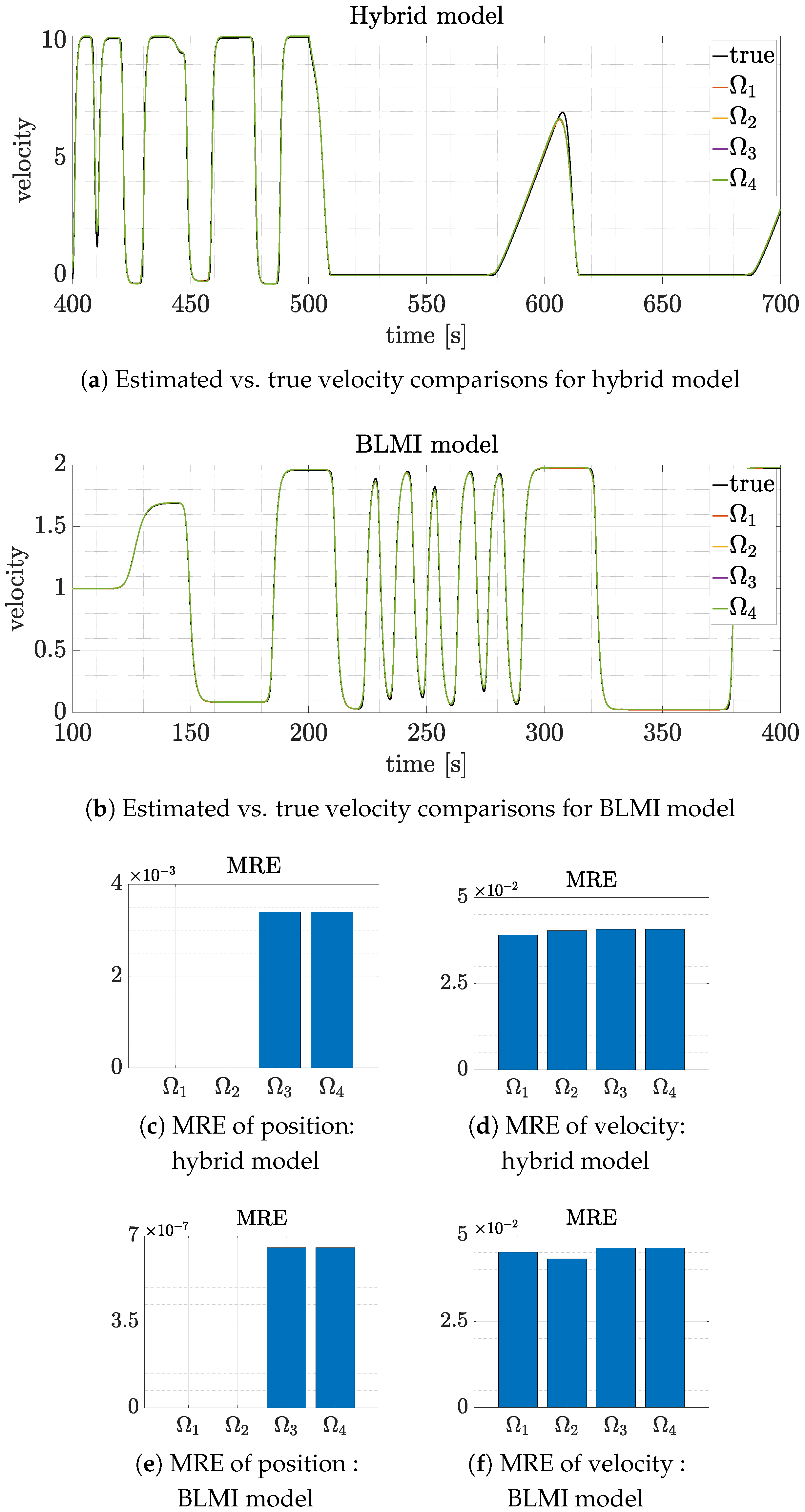
Figure 3 compares the estimated velocity against the ground truth for both the hybrid and BLMI models across all four Ω configurations. The plots in Figure 3a,b are truncated to highlight time intervals where nonlinear behaviors are prominent. As shown in Figure 3a, DMDc successfully captures sharp transitions in the velocity profiles of the hybrid model. Similarly, in Figure 3b, it reproduces the characteristic velocity wave patterns of the BLMI model. These results illustrate the robustness of DMDc in handling a variety of nonlinear dynamics and motivate its application to real-world traffic data.
Notably, the estimated velocity trajectories are nearly identical across all four configurations and closely match the ground truth. To quantify this performance, we compute the mean relative error (MRE) between the estimated and actual states for both position and velocity, as shown in Figure 3c–f. For configurations Ω 3 and Ω 4 , which include position in the state vector, the MRE is reported for both velocity and position. For Ω 1 and Ω 2 , only velocity is estimated, and thus, only the corresponding MRE is shown.
Across both models, the MRE values are consistently low. Position MREs in Figure 3c,e are well below 1% for both the hybrid and BLMI cases, while velocity MREs (Figure 3d,f) remain below 5%. Interestingly, the position MREs in the BLMI model are slightly lower than those in the hybrid model, likely due to the simpler and more consistent dynamics of the former. Overall, the comparable error magnitudes across all configurations and both models confirm the reliability and flexibility of DMDc in modeling car-following dynamics.

3.2.2. Interpreting the DMDc-Estimated Dynamics

To better understand the dynamics learned by DMDc, we analyze the estimated system matrices A ˜ and B ˜ for each state–input configuration Ω across both the hybrid and BLMI models. These matrices are examined alongside their expanded update equations to reveal the structure of the learned dynamics.
  • Case 1: Ω 1
Ω 1 sim = v i Δ v i s i
Estimated hybrid model
A ˜ = 1.0077 B ˜ = 1.1777 0.00191 v ˜ i k + 1 = 0.83 v i k + 0.17777 v i + 1 k 0.00191 s i k v ˜ i k + 1 = 0.00191 x i k + 0.83 v i k 0.00191 x i + 1 k + 0.17777 v i + 1 k
Estimated BLMI model
A ˜ = 1.00543 B ˜ = 0.042808 0.001240 v ˜ i k + 1 = 0.9626 v i k + 0.0428 v i + 1 k 0.00124 s i k v ˜ i k + 1 = 0.00124 x i k + 0.9626 v i k 0.00124 x i + 1 k + 0.0428 v i + 1 k
  • Case 2: Ω 2
Ω 2 sim = v i v i + 1 x i + 1
Estimated hybrid model
A ˜ = 0.8696 B ˜ = 1.17728 0.0000056 v ˜ i k + 1 = 0.8296 v i k + 0.17728 v i + 1 k 0.0000056 x i + 1 k
Estimated BLMI model
A ˜ = 0.9612 B ˜ = 0.0413 0.00000106 v ˜ i k + 1 = 0.9612 v i k + 0.0413 v i + 1 k 0.00000106 x i + 1 k
  • Case 3: Ω 3
Ω 3 sim = x i v i s i Δ v i
Estimated hybrid model
A ˜ = 0.999999 0.200633 0.000006 1.005781 B ˜ = 0.0000951 0.0173629 0.0009592 0.1767054 x ˜ i k + 1 = 0.999904 x i k + 0.183270 v i k 0.000095 x i + 1 k + 0.0173629 v i + 1 k v ˜ i k + 1 = 0.000966 x i k + 0.829076 v i k 0.000959 x i + 1 k + 0.1767054 v i + 1 k
Estimated BLMI model
A ˜ = 0.99999 0.10018 0.00000 1.00369 B ˜ = 0.000023 0.002097 0.000456 0.041933 x ˜ i k + 1 = 1.000013 x i k + 0.098083 v i k 0.000023 x i + 1 k + 0.002097 v i + 1 k v ˜ i k + 1 = 0.000456 x i k + 0.961757 v i k 0.000456 x i + 1 k + 0.041933 v i + 1 k
  • Case 4: Ω 4
Ω 4 sim = x i v i x i + 1 v i + 1
Estimated hybrid model
A ˜ = 0.999904 0.183271 0.000966 0.829075 B ˜ = 0.0000951 0.0173629 0.0009592 0.1767054 x ˜ i k + 1 = 0.999904 x i k + 0.183271 v i k 0.0000951 x i + 1 k + 0.0173629 v i + 1 k v ˜ i k + 1 = 0.000966 x i k + 0.829075 v i k 0.000959 x i + 1 k + 0.1767054 v i + 1 k
Estimated BLMI model
A ˜ = 1.000023 0.098088 0.000455 0.961762 B ˜ = 0.000023 0.002097 0.000456 0.041933 x ˜ i k + 1 = 1.000023 x i k + 0.098088 v i k 0.000023 x i + 1 k + 0.002097 v i + 1 k v ˜ i k + 1 = 0.000455 x i k + 0.961762 v i k 0.000456 x i + 1 k + 0.041933 v i + 1 k
Across all Ω configurations and both models, the estimated velocity dynamics consistently approximate a weighted combination of the subject vehicle’s own velocity v i and that of the leading vehicle v i + 1 , typically taking a form such as
v i k + 1 ρ v i k + ( 1 ρ ) v i + 1 k ,
where ρ 0.83 for hybrid and ρ 0.96 for BLMI. Interestingly, the estimated position updates closely resemble a first-order kinematic relationship, as follows:
x i k + 1 = x i k + v i k Δ t
where Δ t = 0.2 s for the hybrid model and Δ t = 0.1 s for the BLMI model. This result suggests that DMDc captures fundamental motion dynamics with high fidelity, and that the learned models are robust across different Ω constructions, provided that the selected variables are contextually meaningful.
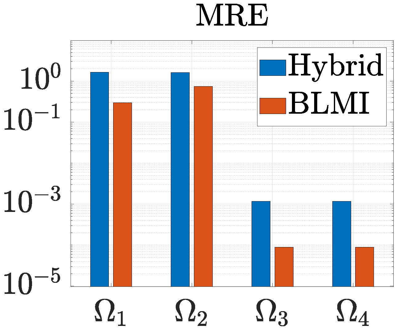
Leveraging this insight, we compute a kinematic position estimate x ^ i for configurations Ω 1 and Ω 2 using their DMDc-estimated velocities v ˜ i . These are then used to derive estimated spacings, which are compared against the true headways. For Ω 3 and Ω 4 , spacing is computed directly from the DMDc-estimated positions x ˜ i . The mean relative errors (MREs) for all configurations are shown in Figure 4.
As shown in Figure 4, spacing estimates based on DMDc-derived positions ( Ω 3 and Ω 4 ) consistently outperform those computed using kinematic approximations ( Ω 1 and Ω 2 ). Additionally, for all configurations, the BLMI model achieves significantly lower spacing MREs than the hybrid model, with errors remaining below unity even in the kinematic cases. This comparative analysis of state–input configurations offers valuable insight into how including or excluding specific variables (e.g., position, relative velocity) influences the accuracy of DMDc-based car-following models, thereby guiding informed variable selection for model development.
These findings highlight the strength of DMDc as a system identification method, capable of capturing and reproducing realistic dynamics across various car-following behaviors. The emergence of near-kinematic update rules provides useful intuition for selecting meaningful state and input variables, especially when applying this framework to real-world traffic datasets.

3.3. DMDc-Based Model Estimation and Prediction Using Real-World Traffic Data

Next, we apply the DMDc framework to real-world car-following data for both estimation and short-term prediction of motion dynamics. The dataset is partitioned into training and testing subsets (refer to the Methods section for further details), where DMDc is first used to estimate the subject vehicle’s velocity dynamics from the training data and then the estimated model is used to predict future states on the testing data. The structure of the state–input vector, Ω , is reiterated for convenience, based on the structure of the available real-world data, which includes relative velocity and spacing along with the velocity of the subject vehicle.
Ω obs = v i Δ v i s i
To estimate spacing, we compute positions kinematically using the DMDc-estimated velocity of the subject vehicle v ˜ i and the known velocity of the leading vehicle v i + 1 . Specifically, the estimated spacing is given by s ^ i = x ^ i + 1 x ^ i , where x ^ i is derived from v ˜ i and x ^ i + 1 is derived from v i + 1 . This approach is applied across all car-following events in the dataset, with the average prediction horizon spanning approximately 8.11 s.
In computing the estimation and prediction metrics, a small number of car-following events were excluded from each dataset. These discarded events exhibit large relative absolute errors ( RAE 1 ), indicating that the DMDc model has failed to reliably estimate or predict the underlying dynamics. Such failures typically occur in cases with too few data points or minimal variation in the driving behavior, which limits the model’s ability to capture meaningful dynamics. Table 2a,b summarize the number of valid events retained and those removed during the estimation and prediction phases, respectively, for each dataset. The HighD and SPMD datasets had the fewest discarded events, likely because their car-following scenarios exhibited sufficient dynamic variation over time. Notably, the HighD and HighD30 datasets were the only ones composed of events with uniform durations, which may have contributed to more consistent model performance.
To assess model performance, we evaluate three key metrics: MRE, MSE, and collision rate, for both estimation and prediction phases. These metrics are computed by aggregating results across all valid car-following events within each dataset. Events exhibiting insufficient data or divergence—such as those with exponential error growth—are excluded by retaining only those cases (valid events) where the relative absolute error (RAE) remains below 1.
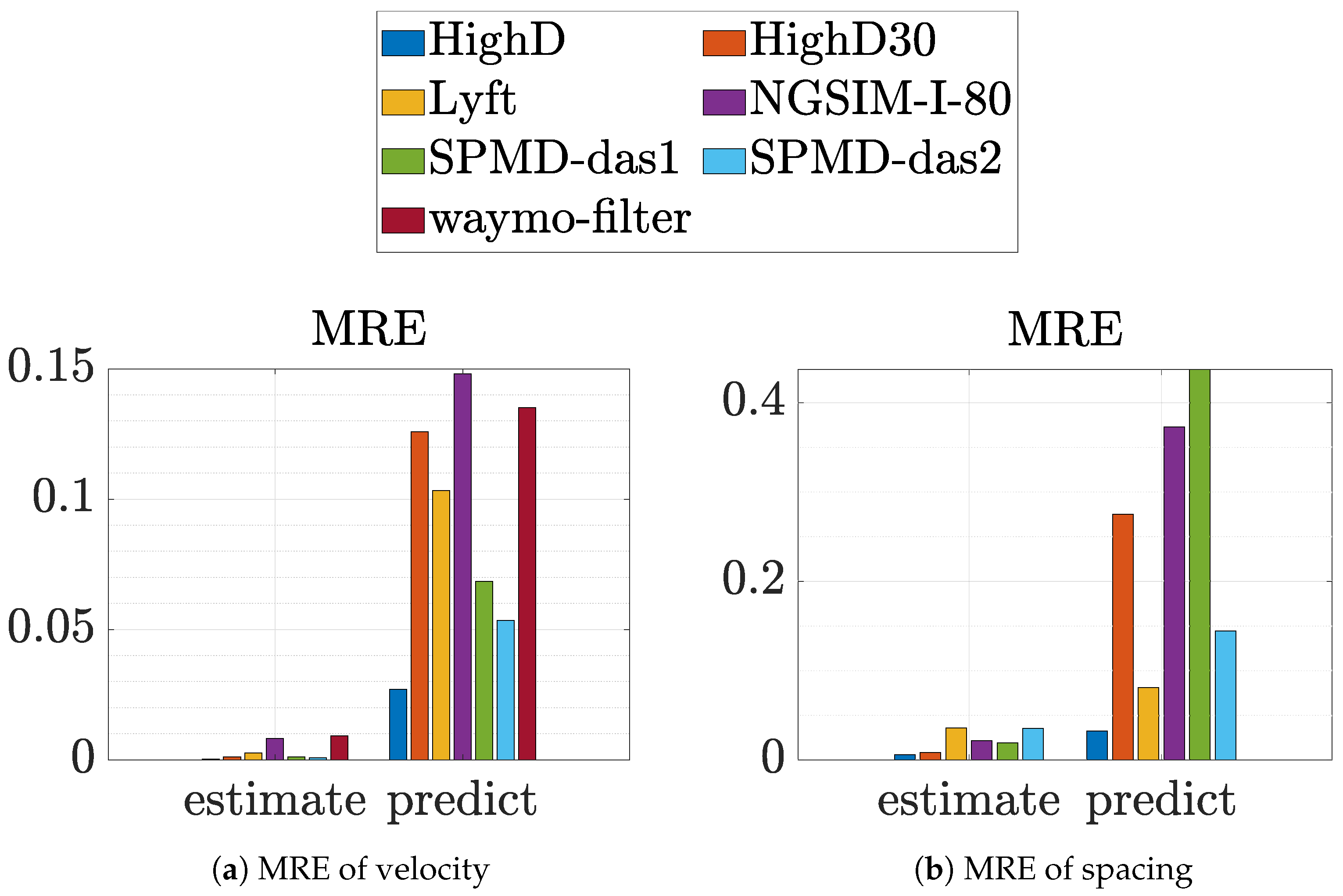
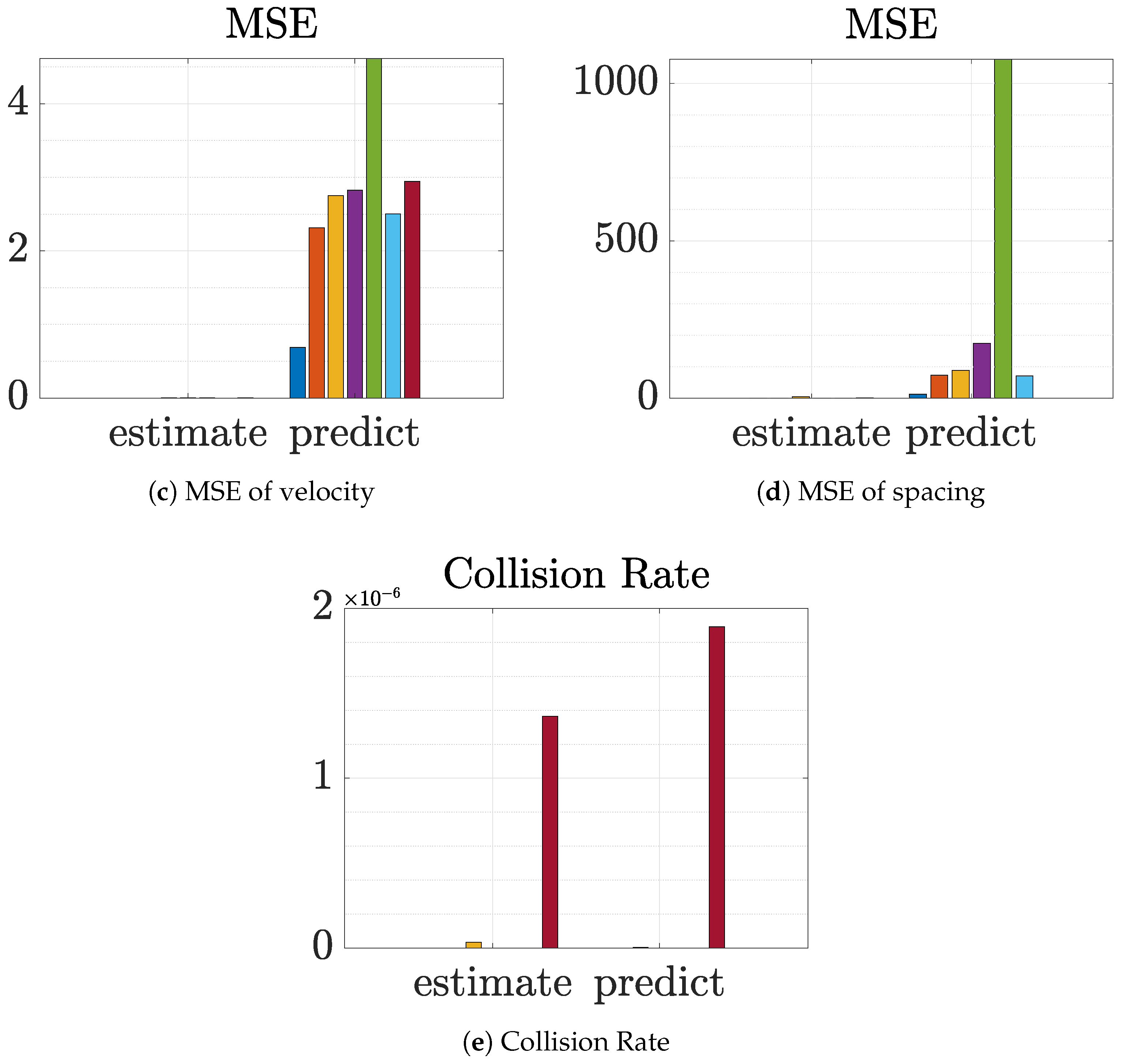
Figure 5a presents the MRE of velocity for both estimation and prediction across the seven datasets. The HighD dataset demonstrates the highest accuracy, with MRE values below 0.2 % during estimation and under 3 % for prediction. Overall, velocity MRE remains below 1 % for estimation and under 15 % for prediction across all datasets, highlighting the robustness of DMDc in capturing and forecasting real-world car-following dynamics. In contrast, spacing MRE results shown in Figure 5b reveal comparatively higher errors, particularly in prediction. While estimation errors for spacing remain within 5 % , prediction errors can reach up to 45 % . This increase likely stems from the fact that spacing is not directly estimated by DMDc but is instead computed through kinematic integration, which can amplify prediction inaccuracies over time.
The MSE results shown in Figure 5c,d further corroborate the trends observed in the MRE analysis. While the relative ranking of datasets varies slightly between MSE and MRE, the HighD dataset consistently produces the most accurate outcomes across both metrics. The MSE values for the estimation phase are consistently and significantly lower than those for the predictive phase, as is typical when forecasting future states from learned dynamics.
Figure 5e illustrates the collision rate, a key safety-related performance metric, for both estimated and predicted trajectories. Given that all the real-world car-following events are collision-free, any instance of predicted negative spacing indicates a physically implausible outcome. Remarkably, DMDc-based predictions result in zero collisions for all datasets except Waymo and Lyft. Even in these exceptions, the collision rates remain extremely low, on the order of O ( 10 6 ) , suggesting that the model’s predictions are largely consistent with physical constraints.
Taken together, these findings validate DMDc as a reliable and interpretable data-driven framework for identifying and forecasting car-following dynamics from real-world observations. The method’s strong performance across multiple real-world datasets highlights its potential utility in traffic modeling, simulation, and control applications.

Temporal Evolution of Prediction Error

To better understand how DMDc-based predictions evolve over time, we analyze the relative absolute error (RAE) across the prediction horizon. This temporal perspective offers insights into the short-term stability and robustness of the learned vehicle dynamics.
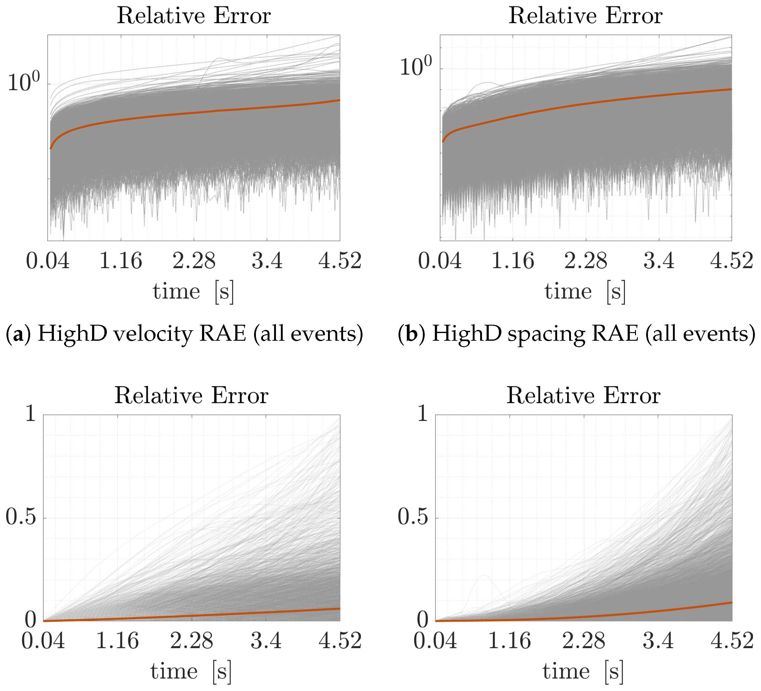
Among all datasets considered, the HighD dataset is unique in providing car-following events of consistent duration—specifically, 113 time steps per event. This consistency allows for a systematic evaluation of how prediction errors accumulate over time. Figure 6 illustrates the temporal progression of relative absolute error (RAE) for both velocity and spacing predictions, shown separately for all events and for a filtered subset of valid events where prediction accuracy satisfies the RAE 1 criterion.
Figure 6a,b display the RAE trajectories over time for all prediction events, with a logarithmic scale used to highlight the impact of a few outlier cases exhibiting large errors. To more accurately reflect the typical prediction performance, Figure 6c,d display the RAE curves limited to valid events ( RAE 1 ), using a linear scale to enhance readability and interpretation.
For these valid events, the average prediction accuracy across events remains high in the initial 1.2 s of forecasting, with both velocity and spacing RAE values close to zero. Thereafter, the average relative error increases gradually, reaching approximately RAE = 0.1 by the end of the 4.52 s prediction window. Notably, spacing errors begin to diverge more rapidly than velocity errors, likely due to the compounding effect of kinematic integration over time. Because DMDc performs prediction in a step-by-step manner, each predicted state serves as the input for the next time step, resulting in the natural accumulation of error over the prediction horizon.
Overall, these findings affirm the stability and effectiveness of DMDc in capturing short-term car-following behavior. The framework accurately models real-world vehicle interactions, maintaining low prediction errors over several seconds of forward simulation.

4. Conclusions and Future Work

This study presents a comprehensive data-driven framework for modeling car-following behavior using conditional transfer entropy for control input identification and dynamic mode decomposition with control for system identification and prediction. By applying CTE to both synthetic and real-world datasets, we demonstrated the ability of information-theoretic measures to uncover latent interaction structures between vehicles. CTE effectively distinguishes between front-only and rear-dominant influence scenarios, guiding the principled selection of state and control input variables for subsequent modeling.
Building on this foundation, we applied DMDc to model and predict car-following dynamics. On simulated datasets—including the hybrid and BLMI models—DMDc produced highly accurate estimates, with position and velocity errors consistently below 1% and 5%, respectively. Remarkably, even with minimal state information, the model effectively captured complex nonlinear behaviors such as stop-and-go waves and abrupt accelerations. Analysis of the estimated system matrices revealed that DMDc naturally discovers underlying kinematic relationships, reinforcing both its interpretability and practical utility.
Extending this approach to real-world datasets, we evaluated the framework across multiple sources of naturalistic driving data. The model achieved strong predictive accuracy, with low mean relative and mean square errors, and maintained physical plausibility with near-zero collision rates. Temporal error analysis further confirmed the short-term stability of DMDc predictions, with minimal deviation over several seconds of forecasting.
To our knowledge, this study marks the first application of DMDc to microscopic traffic modeling and prediction, demonstrating its potential as a powerful tool for data-driven traffic analysis. While prior work using this dataset, such as that of Chen et al. (2023) [11], has focused on calibrating classical car-following models using optimization and machine learning techniques, our approach offers a complementary perspective by constructing interpretable, driver-specific linear models through dynamic mode decomposition with control (DMDc). Unlike machine learning methods that often prioritize predictive performance through population-level generalization, our framework emphasizes individual behavioral dynamics without requiring model-specific assumptions or hyperparameter tuning. This contributes not only to accurate trajectory estimation but also to improved interpretability and model transparency.
The proposed framework offers a lightweight interpretable alternative to black-box learning models, making it suitable for deployment in intelligent transportation systems. Its ability to extract individualized driving dynamics can support applications in adaptive traffic control, behavior prediction, and trajectory planning for autonomous and semi-autonomous vehicles. The model’s linear structure makes it well suited for integration with advanced control strategies. Recent advances in optimal control, particularly model predictive control, have shown strong potential for autonomous and unmanned ground vehicles, where accurate car-following models are critical for trajectory planning and coordination. In this context, our framework offers an interpretable, computationally efficient solution for enabling predictive control in intelligent transportation systems [64,65].
Future work will focus on extending the proposed framework in several directions. First, we aim to incorporate a broader class of traffic events beyond simple car following, including lane changing and merging maneuvers, which will require expanding both the input detection (via CTE or other measures) and the model architecture. Second, we will explore the integration of additional sensing modalities—such as steering and acceleration—into the input space, potentially improving predictive performance in complex traffic scenarios. We have previously introduced a novel framework for collecting experimental driving data using networked driving simulators [66]. This framework provides the foundation for advancing multiple research directions, particularly real-time driver behavior modeling through the application of DMDc techniques developed in the present study. Third, we also plan to use our experimental setup to investigate adaptive or time-varying DMDc formulations to better capture behavioral shifts in nonstationary driving conditions. Finally, the computational time required for processing each car-following event is on the order of milliseconds. Combined with the lightweight nature of DMDc, this motivates future applications in real-time traffic prediction and control [67,68]. Embedding such data-driven models into vehicle-to-vehicle or infrastructure-to-vehicle communication pipelines could support predictive control strategies for autonomous and semi-autonomous driving.

Author Contributions

Conceptualization, S.R.; methodology, S.R. and P.R.; software, S.R. and P.R.; validation, P.R.; formal analysis, P.R. and S.R.; resources, S.R.; data curation, P.R.; writing—original draft preparation, P.R. and S.R.; writing—review and editing, P.R. and S.R.; visualization, P.R.; supervision, S.R.; project administration, S.R.; funding acquisition, S.R. All authors have read and agreed to the published version of the manuscript.

Funding

This work is supported by a National Science Foundation CAREER award (CMMI-2238359).

Data Availability Statement

The simulation dataset is available on request from the authors. The observational data used in this study are sourced from the dataset compiled by Chen et al. in [11], and may be found openly available via GitHub at https://doi.org/10.1038/s41597-023-02718-7.

Conflicts of Interest

The authors declare that they have no known competing financial interests or personal relationships that could have appeared to influence the work reported in this paper. The funders had no role in the design of the study; in the collection, analyses, or interpretation of data; in the writing of the manuscript; or in the decision to publish the results.

References

  1. Xiong, Z.; Hu, P.; Li, N.; Chen, X.; Chen, W.; Wang, H.; Xie, N.; Li, Y.; Dong, C. Modelling and simulation of mixed traffic flow with dedicated lanes for connected automated vehicles. Expert Syst. Appl. 2025, 274, 127027. [Google Scholar] [CrossRef]
  2. Avila, A.M.; Mezić, I. Data-driven analysis and forecasting of highway traffic dynamics. Nat. Commun. 2020, 11, 2090. [Google Scholar] [CrossRef] [PubMed]
  3. Han, J.; Karbowski, D.; Kim, N.; Rousseau, A. Human Driver Modeling Based on Analytical Optimal Solutions: Stopping Behaviors at the Intersections. ASME Lett. Dyn. Syst. Control 2020, 1, 1–8. [Google Scholar]
  4. Treiber, M.; Kesting, A. An Open-Source Microscopic Traffic Simulator. IEEE Intell. Transp. Syst. Mag. 2010, 2, 6–13. [Google Scholar] [CrossRef]
  5. Bando, M.; Hasebe, K.; Nakayama, A.; Shibata, A.; Sugiyama, Y. Dynamical model of traffic congestion and numerical simulation. Phys. Rev. E 1995, 51, 1035–1042. [Google Scholar] [CrossRef]
  6. Treiber, M.; Hennecke, A.; Helbing, D. Congested traffic states in empirical observations and microscopic simulations. Phys. Rev. E 2000, 62, 1805–1824. [Google Scholar] [CrossRef]
  7. Ma, M.; Wang, W.; Liang, S.; Xiao, J.; Wu, C. Improved Car-Following Model for Connected Vehicles Considering Backward-Looking Effect and Motion Information of Multiple Vehicles. J. Transp. Eng. Part A Syst. 2023, 149, 04022148. [Google Scholar] [CrossRef]
  8. Han, J.; Wang, X.; Wang, J.; Shen, C.; Chen, T. Stability Analysis of an Extended Car-Following Model with Consideration of the Surrounding Leading Vehicles and the Rear Vehicle. Appl. Sci. 2025, 15, 4157. [Google Scholar] [CrossRef]
  9. Al Habboush, S.; Yildiz, Y.; Annaswamy, A.M. Human-Inspired Learning for Car Following Models. IFAC-PapersOnLine 2024, 58, 224–229. [Google Scholar] [CrossRef]
  10. Yang, Z.; Jerath, K. Energy-based Data Sampling for Traffic Prediction with Small Training Datasets. IFAC-PapersOnLine 2024, 58, 738–743. [Google Scholar] [CrossRef]
  11. Chen, X.; Zhu, M.; Chen, K.; Wang, P.; Lu, H.; Zhong, H.; Han, X.; Wang, X.; Wang, Y. FollowNet: A Comprehensive Benchmark for Car-Following Behavior Modeling. Sci. Data 2023, 10, 828. [Google Scholar] [CrossRef]
  12. Liu, Y.; Lyu, C.; Zhang, Y.; Liu, Z.; Yu, W.; Qu, X. DeepTSP: Deep traffic state prediction model based on large-scale empirical data. Commun. Transp. Res. 2021, 1, 100012. [Google Scholar] [CrossRef]
  13. Afshari, A.; Lee, J.; Besenski, D.; Dimitrijevic, B.; Spasovic, L. Calibrating Microscopic Traffic Simulation Model Using Connected Vehicle Data and Genetic Algorithm. Appl. Sci. 2025, 15, 1496. [Google Scholar] [CrossRef]
  14. Shi, Y.; Wu, T.; Guo, T.; Huo, J.; Gu, Z.; Dai, Y.; Liu, Z. Traffic simulation optimization considering driving styles. Commun. Transp. Res. 2025, 5, 100181. [Google Scholar] [CrossRef]
  15. Panwai, S.; Dia, H. Neural agent car-following models. IEEE Trans. Intell. Transp. Syst. 2007, 8, 60–70. [Google Scholar] [CrossRef]
  16. Lane, D.; Roy, S. Validating a data-driven framework for vehicular traffic modeling. J. Phys. Complex. 2024, 5, 025008. [Google Scholar] [CrossRef]
  17. Ramlall, P.; Roy, S. Determining critical vehicle connectivity in connected autonomous vehicles using information theory. IFAC-PapersOnLine 2024, 58, 995–1000. [Google Scholar] [CrossRef]
  18. Bishnu, S.K.; Alnouri, S.Y.; Al-Mohannadi, D.M. Computational applications using data driven modeling in process Systems: A review. Digit. Chem. Eng. 2023, 8, 100111. [Google Scholar] [CrossRef]
  19. Habib, M.; Ayankoso, S.; Nagata, F. Data-Driven Modeling: Concept, Techniques, Challenges and a Case Study. In Proceedings of the 2021 IEEE International Conference on Mechatronics and Automation (ICMA), Takamatsu, Japan, 8–11 August 2021; pp. 1000–1007. [Google Scholar]
  20. Solomatine, D.; See, L.; Abrahart, R. Data-Driven Modelling: Concepts, Approaches and Experiences. In Practical Hydroinformatics: Computational Intelligence and Technological Developments in Water Applications; Springer: Berlin/Heidelberg, Germany, 2008; Chapter 2; pp. 17–30. [Google Scholar]
  21. Benner, P.; Breiten, T.; Faßbender, H.; Hinze, M.; Stykel, T.; Zimmermann, R. Model Reduction of Complex Dynamical Systems; Springer: Berlin/Heidelberg, Germany, 2021. [Google Scholar]
  22. Yang, Z.; Jerath, K. Examining the Observability of Emergent Behavior as a Function of Reduced Model Order. In Proceedings of the 2018 Annual American Control Conference (ACC), Milwaukee, WI, USA, 27–29 June 2018; pp. 6218–6223. [Google Scholar]
  23. Schmid, P.J. Dynamic Mode Decomposition and Its Variants. Annu. Rev. Fluid Mech. 2022, 54, 225–254. [Google Scholar] [CrossRef]
  24. Colbrook, M.J. The multiverse of dynamic mode decomposition algorithms. In Numerical Analysis Meets Machine Learning; Handbook of Numerical Analysis; Mishra, S., Townsend, A., Eds.; Elsevier: Amsterdam, The Netherlands, 2024; Volume 25, pp. 127–230. [Google Scholar]
  25. Li, D.; Zhao, B.; Lu, S.; Wang, J. A data-driven method for fast predicting the long-term hydrodynamics of gas–solid flows: Optimized dynamic mode decomposition with control. Phys. Fluids 2024, 36, 103332. [Google Scholar] [CrossRef]
  26. Yu, Y.; Zhang, Y.; Qian, S.; Wang, S.; Hu, Y.; Yin, B. A Low Rank Dynamic Mode Decomposition Model for Short-Term Traffic Flow Prediction. Trans. Intell. Transport. Sys. 2021, 22, 6547–6560. [Google Scholar] [CrossRef]
  27. Proctor, J.L.; Brunton, S.L.; Kutz, J.N. Dynamic Mode Decomposition with Control. SIAM J. Appl. Dyn. Syst. 2016, 15, 142–161. [Google Scholar] [CrossRef]
  28. Proctor, J.L.; Eckhoff, P.A. Discovering dynamic patterns from infectious disease data using dynamic mode decomposition. Int. Health 2015, 7, 139–145. [Google Scholar] [CrossRef]
  29. Dekhici, B.; Benyahia, B.; Cherki, B. Dynamic Mode Decomposition with Control for Data-Driven Modeling of Anaerobic Digestion Process. In Proceedings of the CARI 2022, Tunis, Tunisia, 4–7 October 2022; p. hal-03696038. [Google Scholar]
  30. Hansen, E.; Brunton, S.L.; Song, Z. Swarm Modeling with Dynamic Mode Decomposition. IEEE Access 2022, 10, 59508–59521. [Google Scholar] [CrossRef]
  31. McLean, J.; Fereydoonpour, M.; Ziejewski, M.; Karami, G. Modal Analysis of the Human Brain Using Dynamic Mode Decomposition. Bioengineering 2024, 11, 604. [Google Scholar] [CrossRef]
  32. He, T.; Su, W. A Parametric Dynamic Mode Decomposition for Reduced-Order Modeling of Highly Flexible Aircraft. In Proceedings of the ASME 2024 Aerospace Structures, Structural Dynamics, and Materials Conference, Renton, WA, USA, 29 April–1 May 2024; p. V001T02A010. [Google Scholar]
  33. Wang, X.; Sun, L. Anti-circulant dynamic mode decomposition with sparsity-promoting for highway traffic dynamics analysis. Transp. Res. Part C Emerg. Technol. 2023, 153, 104178. [Google Scholar] [CrossRef]
  34. Schreiber, T. Measuring Information Transfer. Phys. Rev. Lett. 2000, 85, 461–464. [Google Scholar] [CrossRef] [PubMed]
  35. Kaiser, A.; Schreiber, T. Information transfer in continuous processes. Phys. D Nonlinear Phenom. 2002, 166, 43–62. [Google Scholar] [CrossRef]
  36. Sun, J.; Bollt, E.M. Causation entropy identifies indirect influences, dominance of neighbors and anticipatory couplings. Phys. D Nonlinear Phenom. 2014, 267, 49–57. [Google Scholar] [CrossRef]
  37. Varley, T.F.; Pope, M.; Faskowitz, J.; Sporns, O. Multivariate information theory uncovers synergistic subsystems of the human cerebral cortex. Commun. Biol. 2023, 6, 451. [Google Scholar] [CrossRef]
  38. Sattari, S.; Basak, U.S.; James, R.G.; Perrin, L.W.; Crutchfield, J.P.; Komatsuzaki, T. Modes of information flow in collective cohesion. Sci. Adv. 2022, 8, eabj1720. [Google Scholar] [CrossRef]
  39. Butail, S.; Porfiri, M. Detecting Switching Leadership in Collective Motion. Chaos 2019, 29, 011102. [Google Scholar] [CrossRef] [PubMed]
  40. Roy, S.; Howes, K.; Muller, R.; Butail, S.; Abaid, N. Extracting Interactions between Flying Bat Pairs Using Model-Free Methods. Entropy 2019, 21, 42. [Google Scholar] [CrossRef]
  41. Barak-Ventura, R.; Marin, M.R.; Porfiri, M. A Spatiotemporal Model of Firearm Ownership in the United States. Patterns 2022, 3, 100546. [Google Scholar] [CrossRef] [PubMed]
  42. Roy, S.; Abaid, N. Interactional Dynamics of Same-Sex Marriage Legislation in the United States. R. Soc. Open Sci. 2017, 4, 170130. [Google Scholar] [CrossRef]
  43. Marschinski, R.; Kantz, H. Analysing the Information Flow between Financial Time Series. Eur. Phys. J. B-Condens. Matter Complex Syst. 2002, 30, 275–281. [Google Scholar] [CrossRef]
  44. Kesting, A.; Treiber, M.; Helbing, D. General Lane-Changing Model MOBIL for Car-Following Models. Transp. Res. Rec. 2007, 1999, 86–94. [Google Scholar] [CrossRef]
  45. Tadaki, S.i.; Kikuchi, M.; Fukui, M.; Nakayama, A.; Nishinari, K.; Shibata, A.; Sugiyama, Y.; Yosida, T.; Yukawa, S. Phase transition in traffic jam experiment on a circuit. New J. Phys. 2013, 15, 103034. [Google Scholar] [CrossRef]
  46. Nakayama, A.; Kikuchi, M.; Shibata, A.; Sugiyama, Y.; Tadaki, S.i.; Yukawa, S. Quantitative explanation of circuit experiments and real traffic using the optimal velocity model. New J. Phys. 2016, 18, 043040. [Google Scholar] [CrossRef]
  47. Treiber, M.; Kanagaraj, V. Comparing numerical integration schemes for time-continuous car-following models. Phys. A Stat. Mech. Its Appl. 2015, 419, 183–195. [Google Scholar] [CrossRef]
  48. Krajewski, R.; Bock, J.; Kloeker, L.; Eckstein, L. The highD Dataset: A Drone Dataset of Naturalistic Vehicle Trajectories on German Highways for Validation of Highly Automated Driving Systems. In Proceedings of the 2018 21st International Conference on Intelligent Transportation Systems (ITSC), Maui, HI, USA, 4–7 November 2018; pp. 2118–2125. [Google Scholar]
  49. U.S. Department of Transportation Federal Highway Administration. Next Generation Simulation (NGSIM) Vehicle Trajectories and Supporting Data; U.S. Department of Transportation Federal Highway Administration: Washington, DC, USA, 2016. [CrossRef]
  50. Bessina, D.; Sayer, J. Safety Pilot Model Deployment: Test Conductor Team Report; DOT HS; U.S. Department of Transportation Federal Highway Administration: Washington, DC, USA, 2014; Volume 812.
  51. Sun, P.; Kretzschmar, H.; Dotiwalla, X.; Chouard, A.; Patnaik, V.; Tsui, P.; Guo, J.; Zhou, Y.; Chai, Y.; Caine, B.; et al. Scalability in Perception for Autonomous Driving: Waymo Open Dataset. In Proceedings of the 2020 IEEE/CVF Conference on Computer Vision and Pattern Recognition (CVPR), Seattle, WA, USA, 13–19 June 2020; pp. 2443–2451. [Google Scholar]
  52. Houston, J.; Zuidhof, G.; Bergamini, L.; Ye, Y.; Chen, L.; Jain, A.; Omari, S.; Iglovikov, V.; Ondruska, P. One Thousand and One Hours: Self-driving Motion Prediction Dataset. Proc. Mach. Learn. Res. 2021, 155, 409–418. [Google Scholar]
  53. Sattari, S.; Basak, U.S.; Mohiuddin, M.; Toda, M.; Komatsuzaki, T. Inferring the roles of individuals in collective systems using information-theoretic measures of influence. Biophys. Physicobiol. 2024, 21, e211014. [Google Scholar] [CrossRef]
  54. Mwaffo, V.; Keshavan, J.; Hedrick, T.; Humbert, S. A Data-Driven Method to Dissect the Dynamics of the Causal Influence in Complex Dynamical Systems. In Proceedings of the 2018 IEEE Workshop on Complexity in Engineering (COMPENG), Florence, Italy, 10–12 October 2018; pp. 1–5. [Google Scholar]
  55. Butail, S.; Mwaffo, V.; Porfiri, M. Model-free information-theoretic approach to infer leadership in pairs of zebrafish. Phys. Rev. E 2016, 93, 042411. [Google Scholar] [CrossRef]
  56. Bollt, E.M.; Sun, J. Editorial Comment on the Special Issue of “Information in Dynamical Systems and Complex Systems”. Entropy 2014, 16, 5068–5077. [Google Scholar] [CrossRef]
  57. Sipahi, R.; Porfiri, M. Improving on transfer entropy-based network reconstruction using time-delays: Approach and validation. Chaos 2020, 30, 023125. [Google Scholar] [CrossRef] [PubMed]
  58. Lizier, J.T. JIDT: An Information-Theoretic Toolkit for Studying the Dynamics of Complex Systems. Front. Robot. AI 2014, 1, 11. [Google Scholar] [CrossRef]
  59. Kraskov, A.; Stögbauer, H.; Grassberger, P. Estimating mutual information. Phys. Rev. E 2004, 69, 066138. [Google Scholar] [CrossRef] [PubMed]
  60. Roy, S. Quantifying interactions among car drivers using information theory. Chaos 2020, 30, 113125. [Google Scholar] [CrossRef]
  61. Schmid, P.J. Dynamic mode decomposition of numerical and experimental data. J. Fluid Mech. 2010, 656, 5–28. [Google Scholar] [CrossRef]
  62. Kim, G.; Park, C.; Jeong, C.; Kang, C.M.; Cho, J.; Lee, H.; Lee, J.; Kang, D. Vehicle’s Lateral Motion Control Using Dynamic Mode Decomposition Model Predictive Control for Unknown Model. Int. J. Automot. Technol. 2024, 25, 999–1009. [Google Scholar] [CrossRef]
  63. Zhang, X.; Zhang, Y.; Wei, X.; Hu, Y.; Yin, B. Traffic forecasting with missing data via low rank dynamic mode decomposition of tensor. IET Intell. Transp. Syst. 2022, 16, 1164–1176. [Google Scholar] [CrossRef]
  64. Yu, S.; Hirche, M.; Huang, Y.; Chen, H.; Allgöwer, F. Model predictive control for autonomous ground vehicles: A review. Auton. Intell. Syst. 2021, 1, 4. [Google Scholar] [CrossRef]
  65. Akopov, A.S.; Beklaryan, L.A. Agent-Based Modelling of Dynamics of Interacting Unmanned Ground Vehicles Using FLAME GPU. Program. Comput. Softw. 2024, 50, S91–S103. [Google Scholar] [CrossRef]
  66. Ramlall, P.; Jones, E.; Roy, S. Development of a Networked Multi-Participant Driving Simulator with Synchronized EEG and Telemetry for Traffic Research. Systems 2025, 13, 564. [Google Scholar] [CrossRef]
  67. Shabab, K.R.; Mustavee, S.; Agarwal, S.; Zaki, M.H.; Das, S.K. Dynamic mode decomposition type algorithms for modeling and predicting queue lengths at signalized intersections with short lookback. J. Intell. Transp. Syst. 2024, 28, 741–755. [Google Scholar] [CrossRef]
  68. Das, S.; Mustavee, S.; Agarwal, S.; Hasan, S. Koopman-Theoretic Modeling of Quasiperiodically Driven Systems: Example of Signalized Traffic Corridor. IEEE Trans. Syst. Man Cybern. Syst. 2023, 53, 4466–4476. [Google Scholar] [CrossRef]
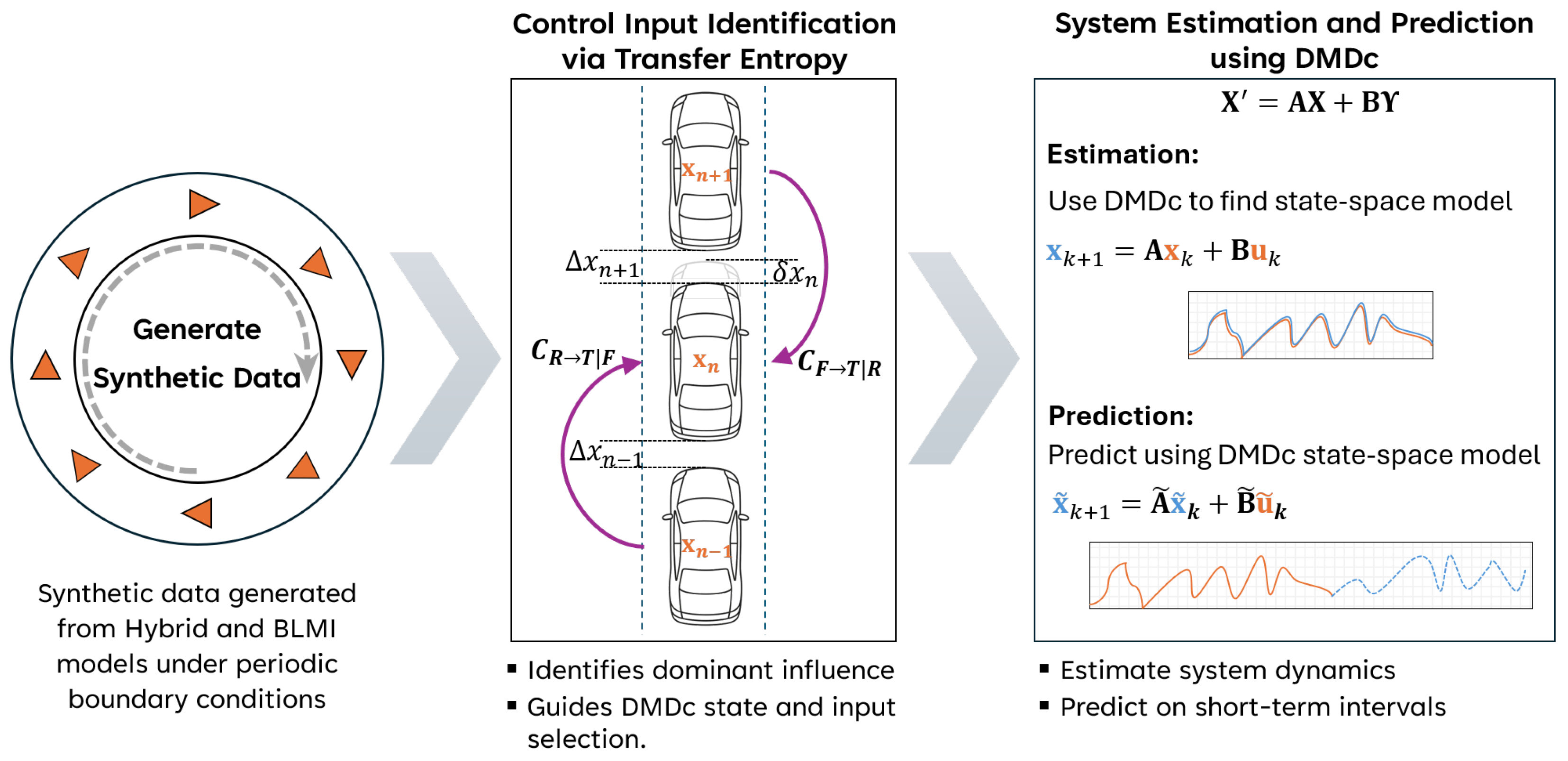
Figure 1. Overview of the proposed data-driven modeling framework. The process consists of two main steps: (1) identifying directional inter-vehicle influence using CTE on synthetic model data to select relevant control inputs and (2) applying DMDc to estimate and predict car-following dynamics for real-world car-following data.
Applsci 15 09700 g001
Figure 2. Results of conditional transfer entropy for the hybrid model and the BLMI model with p = 1 (no rear influence) and p = 0.2 (dominant rear influence).
Applsci 15 09700 g002
Figure 3. Estimated vs. true simulated velocities for the (a) hybrid model and (b) BLMI model when p = 1 (no rear influence) for each Ω . The position and velocity MRE for each case are shown for the (c,d) hybrid and (e,f) BLMI models, respectively.
Applsci 15 09700 g003
Figure 4. Mean relative error (MRE) of spacing estimates for each configuration of Ω in the hybrid and BLMI models.
Applsci 15 09700 g004
Figure 5. MRE, MSE, and collision rate for DMDc estimation and prediction on real-world car-following data.
Applsci 15 09700 g005
Figure 6. Time evolution of prediction RAE for velocity and spacing in the HighD dataset. The gray dashed lines represent individual events; the solid orange line denotes the average RAE across valid events.
Applsci 15 09700 g006
Table 1. Simulation parameters.
(a) BLMI model simulation parameters
ParameterValue
number of vehiclesN100
simulation time step (s) Δ t 0.1
simulation time (s) T sim 5000
track length (m) L track 400
BLMI
ParameterValue
σ BLMI 0.8
m1
λ 0
p 1 , 0.2
h c 4
v max F 2
v max B 2
(b) Hybrid model simulation parameters
ParameterValue
number of vehiclesN30
simulation time step (s) Δ t 0.01
simulation time (s) T sim 2500
track radius (km) R r i n g 50
OVMIDM
ParameterValueParameterValue
σ OVM 1.8 a max 0.3
α 5.5 v 0 30
β 0.37 δ 4
s 0 9.1 s 0 2
v 0 4.9 Δ T 1.5
b3
l v 5
Table 2. Number of valid events considered in each dataset when calculating average DMDc estimation and prediction metrics.
(a) Estimation
Dataset# events# valid events% valid events
HighD12,54112,54099.992
HighD301319130098.559
Lyft24,09321,91090.939
NGSIM1930177992.176
SPMD-das116,65816,658100
SPMD-das224,24724,24699.996
Waymo144084858.889
(b) Prediction
Dataset# events# valid events% valid events
HighD12,54112,46899.418
HighD301319120891.585
Lyft24,09320,01983.091
NGSIM1930169387.720
SPMD-das116,65815,66994.063
SPMD-das224,24723,54897.117
Waymo144072650.417
Disclaimer/Publisher’s Note: The statements, opinions and data contained in all publications are solely those of the individual author(s) and contributor(s) and not of MDPI and/or the editor(s). MDPI and/or the editor(s) disclaim responsibility for any injury to people or property resulting from any ideas, methods, instructions or products referred to in the content.