Article

Hybrid Hourly Solar Energy Forecasting Using BiLSTM Networks with Attention Mechanism, General Type-2 Fuzzy Logic Approach: A Comparative Study of Seasonal Variability in Lithuania

by
Naiyer Mohammadi Lanbaran
*,
Darius Naujokaitis
,
Gediminas Kairaitis
and
Virginijus Radziukynas
Smart Grids and Renewable Energy Laboratory, Lithuanian Energy Institute, Breslaujos St. 3, 44403 Kaunas, Lithuania
*
Author to whom correspondence should be addressed.
Appl. Sci. 2025, 15(17), 9672; https://doi.org/10.3390/app15179672
Submission received: 30 July 2025 / Revised: 29 August 2025 / Accepted: 29 August 2025 / Published: 2 September 2025

Abstract

This research introduces a novel hybrid forecasting framework for solar energy prediction in high-latitude regions with extreme seasonal variations. This approach uniquely employs General Type-2 Fuzzy Logic (GT2-FL) for data preprocessing and uncertainty handling, followed by two advanced neural architectures, including BiLSTM and SCINet with Time2Vec encoding and Variational Mode Decomposition (VMD) signal processing. Four configurations are systematically evaluated: BiLSTM-Time2Vec, BiLSTM-VMD, SCINet-Time2Vec, and SCINet-VMD, each tested with GT2-FL preprocessed data and raw input data. Using meteorological data from Lithuania (2023–2024) with extreme seasonal variations where daylight hours range from 17 h in summer to 7 h in winter, F-BiLSTM-Time2Vec achieved exceptional performance, with nRMSE = 1.188%, NMAE = 0.813%, and WMAE = 3.013%, significantly outperforming both VMD-based variants and SCINet architectures. Comparative analysis revealed that Time2Vec encoding proved more beneficial than VMD preprocessing, especially when enhanced with fuzzification. The results confirm that fuzzification, BiLSTM architecture, and Time2Vec encoding provide the most robust forecasting capability under various seasonal conditions.

1. Introduction

Energy consumption drives economic progress and prosperity, including electricity generation and industrial usage. Currently, fossil fuels remain the primary global energy source [1]. As a result, the increasing recognition of the necessity for energy conservation and the adoption of alternative sources, particularly renewable energy (RE), has intensified in response to escalating concerns regarding greenhouse gas (GHG) emissions and climate change. While renewable energy refers to naturally replenishing sources like solar and wind, sustainable energy represents a broader approach that includes both renewable sources and efficient energy distribution systems. This comprehensive model enables society to generate and utilize energy while minimizing environmental impacts and resource depletion [2]. Among the renewable options, solar energy has been recognized as a crucial component in addressing these energy requirements [3,4]. Solar power in the European Union grew dramatically from 7.4 Terawatt hours (TWh) (1% of electricity mix) in 2008 to 252.1 TWh (approximately 8.5%) in 2023, representing a 34-fold increase [5]. Innovative grid initiatives aim to substantially increase the proportion of renewable energy in the grid, particularly in regions with high seasonal variability [6].
Despite impressive growth in renewable energy, a key challenge in integrating sources like solar and wind into the power grid is the intermittent nature of their electricity production, which is beyond human control. Successfully incorporating solar energy depends heavily on accurately forecasting its power generation and leveraging hybrid systems that combine solar and wind to improve grid reliability and accessibility [7]. Consequently, the accurate prediction of future RE availability is crucial, enabling the grid to allocate producers to meet fluctuating demand efficiently. This rapid expansion has further heightened the importance of accurate forecasting for power generation, enabling electric operators to maintain a precise balance between production and consumption [5,6,7].

1.1. Photovoltaic Forecasting Challenges

The increasing global demand for integrating RE, particularly solar power, into power grids highlights the economic and technological challenges associated with the increased penetration of flat-panel photovoltaic (PV), concentrated solar power (CSP), and concentrated photovoltaic (CPV) systems. These challenges stem from solar resource variability, seasonal production fluctuations, costly energy storage, and the need to balance grid flexibility and reliability [8]. These challenges are particularly acute in Lithuania, where seasonal differences in solar radiation are substantial, with daylight hours ranging from 17 h in summer to only 7 h in winter. Rodríguez et al. [9] demonstrated that solar plants frequently require support from ancillary generators during high variability, increasing capital and operational costs.
Solar energy generation forecasting has evolved from basic monitoring systems using inverter-based data collection [10,11,12] to sophisticated methodologies employing statistical models, satellite imaging, Numerical Weather Prediction, and hybrid artificial neural networks for day-ahead market integration [13]. Enhanced forecasting methods are essential for power system operators’ unit commitment planning and reserve capacity management. Forecasting methods are categorized into direct models (using historical PV output and meteorological data) and indirect models (predicting solar irradiation at PV locations), with direct methods generally demonstrating superior performance [14,15].
Weather-related uncertainties significantly impact solar energy forecasting accuracy. Atmospheric conditions, including dust, moisture, aerosols, clouds, and temperature variations, create substantial prediction challenges, with clouds potentially reducing solar energy by up to 100% on heavily overcast days [16,17]. Fuzzy logic-based (FL) models address these uncertainties by incorporating meteorological parameters such as latitude, longitude, altitude, seasonal variations, sunshine duration, and temperature [18]. Type-2 Fuzzy Logic (T2-FL) systems offer enhanced uncertainty handling compared to traditional Type-1 systems, providing additional degrees of freedom for direct uncertainty modeling [19,20].

1.2. State-of-the-Art Review

Deep learning (DL) has emerged as a powerful approach for solar energy forecasting since Geoffrey Hinton’s breakthrough work in 2006 [21]. Traditional fully connected networks struggle with temporal dependencies, leading to specialized architectures including Recurrent Neural Networks (RNNs), Long Short-Term Memory (LSTM), and bidirectional LSTM (BiLSTM) networks that effectively capture time-series patterns [22,23,24]. Recent architectural innovations include Temporal Convolutional Networks (TCN), Sample Convolution, and Interactive Neural Networks (SCINet). TCN implementations have demonstrated 20–30% accuracy improvements in 6-h PV forecasting [25,26].
Advanced hybrid models have emerged as promising solutions. Kong et al. introduced a solar radiation prediction model using TCN with attention [27], while Liu et al. developed enhanced TCN-DenseNet architectures demonstrating significant MAPE reductions [28]. Limouni et al. proposed hybrid LSTM-TCN models that outperformed individual architectures under various seasonal conditions [29]. Recent developments in VMD-based models have shown remarkable progress, with studies reporting improved performance in seasonal forecasting [30]. Advanced architectures, including Generative Adversarial Network BiLSTM (GAN-BiLSTM) [31], VMD-CNN-BiGRU (Gated Recurrent Unit) [32], VMD-Transformer models [33,34], and PSO-BiLSTM [35], have established new benchmarks, with recent models achieving error rates below 15% and accuracy rates up to 98.5%. Table 1 Comparative Overview of Solar Forecasting Approaches.

1.3. Research Gaps and Motivation

Despite significant advances in solar forecasting methodologies, three critical limitations prevent effective deployment in extreme seasonal climates:
Seasonal Variability Challenge: Most existing studies focus on regions with moderate seasonal variations. High-latitude regions like Lithuania (54° N–56° N) with extreme seasonal patterns (17-h summer days vs. 7-h winter days) present unique forecasting challenges that current methodologies inadequately address, with performance degradation exceeding 40% during seasonal transitions.
Uncertainty Integration Gap: While individual fuzzy logic and deep learning approaches exist, systematic integration of advanced uncertainty quantification (GT2-FL) with state-of-the-art neural architectures (BiLSTM, SCINet) remains unexplored for enhanced uncertainty handling in complex seasonal environments.
Architectural Optimization Deficiency: Comparative studies of advanced architectures (BiLSTM vs. SCINet) with different preprocessing techniques (Time2Vec vs. VMD) under varying seasonal conditions are lacking, limiting optimal model selection for specific climate conditions.
Implementation-Research Divide: Most research focuses on theoretical improvements without addressing real-world deployment challenges in regions with high meteorological variability, creating a significant gap between laboratory performance and operational reliability.

1.4. Research Contributions and Theoretical Significance

This study addresses these fundamental limitations through a novel hybrid methodology that advances the theoretical understanding and practical implementation of solar energy forecasting in climatically challenging regions. The key contributions include the first comprehensive implementation employing General Type-2 Fuzzy Logic (GT2-FL) for data preprocessing and uncertainty handling, followed by advanced deep learning architectures (BiLSTM and SCINet) enhanced with specialized preprocessing techniques (Time2Vec and VMD), providing a theoretical foundation for uncertainty-aware deep learning in renewable energy forecasting.
Systematic Architectural Analysis: Comprehensive evaluation of four distinct model configurations: BiLSTM with Time2Vec, BiLSTM with VMD, SCINet with Time2Vec, and SCINet with VMD, each tested in both fuzzified and non-fuzzified variants under realistic seasonal variations, enabling evidence-based architectural selection.
Advanced Uncertainty Modeling: Integration of GT2-FL preprocessing pipeline with Karnik-Mendel type-reduction and single-centroid defuzzification for enhanced uncertainty management in volatile weather conditions, addressing the theoretical gap in uncertainty quantification for renewable energy systems.
Seasonal Adaptation Methodology: Comprehensive evaluation across spring/summer and fall/winter periods using data from Lithuania (2023–2024), providing empirical insights for high-latitude regions with similar climate patterns and establishing performance benchmarks for extreme seasonal environments.
Operational Implementation Strategy: Development of a rolling forecasting strategy using 24-h actual data windows with hourly predictions, preventing error propagation while maintaining real-world applicability, bridging the gap between research and operational deployment.
This research advances the scientific understanding of uncertainty-aware renewable energy forecasting while providing practical solutions for challenging geographical conditions with extreme seasonal variations. The integrated approach demonstrates how a systematic combination of fuzzy logic, advanced neural architectures, and specialized preprocessing can address the complex temporal patterns and uncertainty inherent in solar energy generation.
The remainder of this paper is organized as follows: Section 2 presents the theoretical background and mathematical foundations. Section 3 delineates the proposed model architecture and preprocessing methodologies. Section 4 presents comprehensive results and performance analysis. Section 5 provides a detailed discussion of findings and their implications. Section 6 offers conclusions and future research directions.

2. Theoretical Background

This section provides essential theoretical foundations for the proposed hybrid methodology, focusing on key components that distinguish our approach from existing forecasting methods.

2.1. Preprocessing Techniques

2.1.1. General Type-2 Fuzzy Logic Systems

Complex forecasting challenges involve multiple sources of uncertainty, including incomplete data, inaccuracies, ambiguity, and conflicting evidence. Type-1 Fuzzy Sets (T1-FSs) use fixed membership values between 0 and 1 but have limitations when handling multidimensional uncertainties. Equation (1) represents the T-1FS membership function [46]. Type-2 Fuzzy Sets (T2-FSs) overcome these constraints by treating membership functions as fuzzy sets rather than crisp values, providing enhanced uncertainty modeling capabilities [47].
T2-FSs are created by “blurring” T1-FS membership functions, resulting in three-dimensional representations that can model “uncertainty about uncertainty” [48,49]. While T1-FL systems provide precise membership degrees (0 to 1) for input variables, T2-FSs offer more robust handling of the complex ambiguities inherent in solar forecasting applications, where weather conditions create multiple layers of uncertainty that traditional fuzzy systems cannot adequately address.
T1-FL gives exact membership values for all x A , with a membership degree of μ A x , while T2-FL models the uncertainty in those membership values, making it better suited for solar forecasting applications with complex, overlapping uncertainties.
μ A x =     0                                                                                                                                                                     i f   x A     1                                                                                                                                                                     i f   x A V a l u e   b e t w e e n   ( 0 ,   1 )                                 f o r   i n t e r m e d i a t e   d e g r e e s   o f   m e m b e r s h i p
Figure 1 illustrates the Type-1 Fuzzy Gaussian membership function formulated by the authors, which is the foundational component for modeling uncertainty in the fuzzy system. General Type 2- Fuzzy Set A ~ in the universe of discourse X is defined as an Equation (2):
A ~ =   x , u , μ A ~ x , u x X , u J x 0,1
where u indicates the uncertainty, x X is a component of the domain X , u J x 0,1 is the secondary variable (secondary membership degree), μ A ~ x , u is the secondary membership function of the T-2FS at x and u , and J x is the footprint of uncertainty (FOU) at x , representing the range of secondary membership degrees. The primary membership function μ A ~ ( x ) maps x to a fuzzy set in the interval [ 0,1 ] , not just a single value. In other words, for each x , you obtain a range of membership degrees J x .
The secondary membership function μ A ~ x , u specifies the degree to which each value of u belongs to the fuzzy set at x .
The membership function of a GT2FS is a surface in 3D, where the X-axis represents the Primary Domain, the Y-axis represents the Secondary Domain, and the Z-axis represents the membership degree μ A ~ x , u .
GT2FS provides a more comprehensive depiction of uncertainty by capturing variability in primary memberships and uncertainty about the precise value of membership degrees (via secondary membership). This makes it handy for applications with complicated uncertainty that T1-FSs cannot handle alone [49].
Figure 2 demonstrates a 3D surface plot of a General Type-2 fuzzy set using Gaussian membership functions. The plot illustrates the primary domain (x-axis) and secondary domain (y-axis), with the height (z-axis) representing the fuzzy membership values. The Gaussian shape captures both the primary membership and the uncertainty in the secondary membership values, providing a detailed representation of fuzzy uncertainty.

2.1.2. Time to Vector

The Time2Vec embedding layer offers a fundamental vector representation of time well-suited for numerous deep learning models. This layer can detect periodic and non-periodic patterns automatically, enhancing prediction accuracy [50]. Given a time series τ , the Time2Vec representation of the τ time scalar is expressed as t 2 v ( τ ) , a vector of length k + 1 , which is defined in Equation (3):
t 2 v τ i = ω 0 h τ   +   φ 0 h ,                     i f   i = 0     sin ω i h τ + φ i h ,             i f   1 i k
where t 2 v τ i represents the i t h feature of t 2 v τ . The parameters ω i h and φ i h are learnable. The linear function ω 0 h τ + φ 0 h captures the non-periodic elements of the time series. The periodic components of the input data are obtained through the periodic activation function sin ω i h τ + φ i h [50].

2.1.3. Variational Mode Decomposition (VMD)

The VMD layer provides fundamental frequency-domain analysis of signals, particularly suited for complex signal processing tasks. This layer integrates Wiener filtering, Hilbert transform, and frequency mixing to decompose signals into Intrinsic Mode Function (IMF) components, enhancing solar irradiance prediction accuracy through effective noise reduction and adaptive bandwidth optimization [51,52]. The algorithm addresses a variational problem mathematically formulated in Equations (4) and (5).
m i n u k , { w k } k t [ δ t + j π t u k t ] e j w k t 2 2
S . t . k u k = χ
Here { u k } represents the collection of all modes, and { w k } represents their associated central frequencies. The original input signal is denoted by χ , while k indicates the total number of modes. Additionally, t represents the gradient regarding time, δ t represents an impulse function, j represents the imaginary unit, and the symbol indicates the convolution operation.

2.1.4. Sine-Cosine Transformation

Time-series decomposition breaks data into trend, seasonal, and residual components, allowing the model to learn these aspects separately. This decomposition is mathematically expressed in Equation (6) for an additive model.
Y t = T t + S t + R t
Y t is the observed value, T t is the trend, S t is the seasonal component, and R t is the residual. This technique helps isolate long-term trends and cyclic behaviors, improving the model’s focus on the residual data for better prediction accuracy. Cyclical time features such as hour of day, day of week, and month are encoded using sine-cosine transformations to preserve their periodicity. Cyclical time features such as hour of day, day of week, and month are encoded using sine-cosine transformations to preserve their periodic nature [53]. For a cyclical feature x with a period T , the transformation is defined in Equations (7) and (8) as:
x s i n = s i n ( 2 π x T )
x c o s = c o s ( 2 π x T )
This encoding ensures smooth transitions across periodic boundaries and enables the model to capture recurring patterns such as daily and seasonal solar generation cycles. These patterns are crucial for accurate forecasting in high-latitude regions with extreme seasonal variations.

2.1.5. Attention Mechanism

Attention mechanisms enable models to focus on relevant temporal segments by computing weighted combinations of input features [54]. For an input sequence, the attention output is calculated as in Equations (9)–(11):
S q , k i = q T k i
α i = e x p ( s q , k i ) j = 1 n e x p ( s q , k i )
z = i = 1 n α i v i
For an input sequence of length n , let the query vector q , key vectors k i , and value vectors v i be the main elements of the attention mechanism. Query vector q represents the current position or task the model tries to predict. Key vectors k i represent different parts of the input sequence, and value vectors v i contain the actual information of the sequence elements. S q , k i the attention score computes the similarity between the query and keys (dot product). α i represents attention weights that normalize scores using softmax, and z is the attention output that computes a weighted sum of values [55].

2.2. Main Forecasting Models

2.2.1. Bidirectional Long Short-Term Memory (BiLSTM)

BiLSTM networks process information forward and backward directions, enabling comprehensive capture of temporal dependencies in time series data [56]. The architecture consists of two LSTM layers processing each input’s sequence in opposite directions. BiLSTM processes information in both directions, enabling the model to capture context from past and future time steps for each input. x t , enhancing its understanding of sequential data. Equations (12)–(14) define the forward hidden vector. h i , the backward hidden vector h i , and the output h i .
h i = L S T M x i , i 1 , n
h i = L S T M x i , i n , 1
h i = h i , h i , i n , 1

2.2.2. Sample Convolution and Interactive Neural Networks (SCINet)

The SCINet model follows an encoder–decoder framework [57]. The encoder consists of a hierarchical convolutional network that uses various convolutional filters to capture dynamic temporal dependencies across multiple resolutions. Its core component is the SCI-Block, which processes an input sequence. F Through a structured downsample-convolve-interact process. Then input F is split into two sub-sequences:
  • F o (odd-indexed elements)
  • F e (even-indexed elements)
The sub-sequences undergo a two-step interactive learning process to share information and prevent loss from downsampling, as shown in Equation (15). Then we have information Fusion that is presented in Equation (16):
F o s = F o exp Φ F e   a n d   F e s = F e exp Ψ F o
F ´ o = F o s ± ρ F e s   a n d   F ´ e = F e s ± η F o s
where Φ , Ψ , ρ , and η are 1D convolutional modules, is the element-wise product, and exp is the exponential function.
Multiple SCI-Blocks are arranged in a binary tree to form the encoder, capturing multi-scale temporal patterns. The processed features are then rearranged and passed to a fully connected decoder to generate forecasts [58].

2.3. Evaluation Metrics

Model performance is assessed using three key metrics specifically chosen for solar forecasting applications:
  • Normalized Root Mean Squared Error (nRMSE%): Based on maximum observed power, emphasizing larger errors
  • Normalized Mean Absolute Error (NMAE%): Based on plant capacity, providing a reliable accuracy measure
  • Weighted Mean Absolute Error (WMAE%): Based on total energy production, accounting for generation-weighted errors
These metrics collectively provide a comprehensive assessment of forecasting accuracy across different operational scenarios and seasonal conditions [59].
In Equations (17)–(19):
The normalized mean absolute error NMAE%, based on the plant’s net capacity C .
N M A E % = 1 N k = 1 N P m , k P p , k C . 100
where N denotes the number of samples (hours) considered, typically a day, month, or year. For this metric, the rated power of the PV system was used as C .
The weighted mean absolute error W M A E % , based on the total energy production:
W M A E % = k = 1 N P m , k P p , k k = 1 N P m , k . 100
The normalized root means square error n R M S E % , based on the maximum observed power generated:
n R M S E % = k = 1 N P m , k P p , k 2 N m a x ( P m , k ) . 100
Here, P m , k is measured power and forecasted power P p , k   at   hour   k . NMAE% is commonly used to evaluate prediction accuracy because it mitigates the bias seen in WMAE% when dealing with small power values. It weights errors relative to capacity C , offering a more reliable measure. RMSE% measures the average magnitude of absolute hourly errors, emphasizing more significant errors to highlight particularly undesirable results [59].

3. Proposed Model Architecture

3.1. Forecasting Scope and Temporal Framework

This study implements short-term photovoltaic power forecasting with 1-h ahead predictions, classified within the standard renewable energy forecasting taxonomy (30 min to 6 h ahead). The methodology employs 24-h rolling historical data windows, designed explicitly for high-latitude regions with extreme seasonal variations.
Temporal Specifications: The forecast horizon is 1 h ahead (short-term classification). The input window (looking back) is 24 h of historical data. The update frequency is hourly forecasts. In terms of geographical focus, we consider Lithuania’s extreme seasonal conditions (17-h summer vs. 7-h winter daylight).

3.2. Data Description and Implementation Details

In this study, we designed an hourly forecast of solar energy generation in Lithuania, employing daytime data from 1 January 2023, to 31 August 2024. The meteorological data (forecasted meteo elements) used in this research were obtained from the Lithuanian Hydrometeorological Service (LHMT) through their API (https://api.meteo.lt/) (accessed on 5 September 2024). The model incorporates 28 distinct input features, encompassing meteorological parameters, derived solar radiation components, decomposed power signals, temporal encodings, and historical power values. The inherent variability and uncertainty in solar energy data present significant challenges, which we managed by developing a novel methodology based on combining GT2-FL and advanced deep learning models, incorporating comprehensive feature engineering and time series decomposition techniques.
All models were implemented using Python 3.12.7 with TensorFlow 2.19.0 and Keras 3.9.2 frameworks. Experiments were conducted on a high-performance workstation equipped with an Intel i7 processor running at 2.32 GHz, 31.7 GB of RAM (11.6 GB used, 37% utilization), Intel UHD Graphics with 7% usage, and a Samsung NVMe SSD with 1% active time. The training process utilized the Adam optimizer with a learning rate of 0.001 and the Huber loss function. Data was chronologically split into 70% for training (January–August 2023), 15% for validation (August 2023–June 2024), and 15% for testing (June–August 2024).

3.3. Data Preprocessing Pipeline

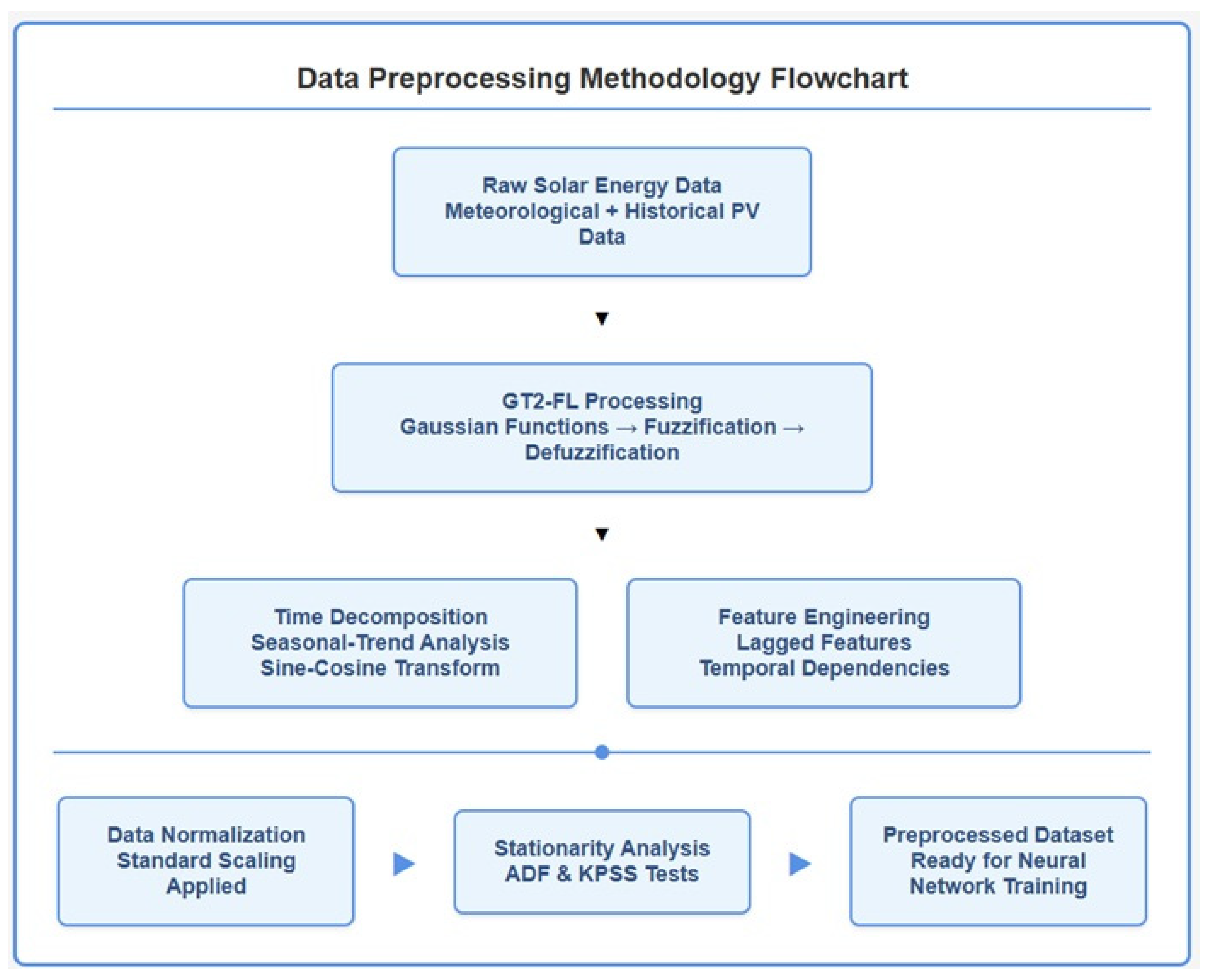
Figure 3 illustrates the comprehensive data preprocessing methodology employed in this study.

3.3.1. Fuzzification and Defuzzification

General Type-2 Fuzzy Logic preprocessing is applied to address uncertainty in solar energy data using Gaussian membership functions. The fuzzification process transforms crisp inputs into fuzzy sets with primary and secondary domains as linearly spaced arrays in [0, 1]. Type-reduction employs the Karnik-Mendel algorithm followed by single-centroid defuzzification, which is selected for computational efficiency when input values across features are proximate.

3.3.2. Temporal Feature Engineering and Preprocessing Workflow

The preprocessing workflow combines multiple techniques:
  • Time Series Decomposition: Solar power data is decomposed into trend, seasonal, and residual components using additive decomposition Y t = T t + S t + R t .
  • Cyclical Feature Encoding: Time-related variables undergo sine-cosine transformations to preserve the periodic nature and enable the recognition of recurring patterns.
  • Lagged Features: Historical data from previous time steps are incorporated to capture temporal dependencies, using actual measurements rather than predicted values during rolling forecasting.
  • Normalization: Standard scaling ensures all features operate on comparable scales, preventing numerical instability during training.

3.3.3. Stationarity and Statistical Analysis

Stationarity assessment is crucial for understanding time series properties and their suitability for forecasting models. A time series is considered stationary when its statistical properties (mean, variance, and covariance) remain constant over time, making it generally easier to model and forecast due to predictable statistical behavior [60,61].
Our methodology employed complementary statistical tests: the Augmented Dickey–Fuller (ADF) test (null hypothesis: non-stationarity) and the Kwiatkowski-Phillips-Schmidt-Shin (KPSS) test (null hypothesis: stationarity). Statistical significance was determined using p-values compared to 0.05.
Analysis revealed that the original PV power generation series exhibits inherent non-stationarity, confirmed by conflicting test results (ADF: stationary with p-value 0.0000; KPSS: non-stationary with p-value 0.0100). This statistical conflict indicates complex nonstationary components in solar power generation data.
The decomposition approaches demonstrated varying effectiveness in transforming components into stationary series:
Decomposed residuals: Achieved true stationarity across all models
VMD-based models: Transformed 42.9% of components (3 out of 7) into stationary series, representing a significant advantage
Cyclical features: Retained non-stationary characteristics, reflecting inherent variability in solar generation patterns
This selective stationarity aligns with our modeling strategy, enabling effective handling of both deterministic (stationary) and stochastic (non-stationary) components while accounting for uncertainty through Type-2 fuzzy modeling.

3.3.4. Meteorological Impact Integration

Correlation analysis between weather parameters and PV output demonstrates strong dependencies, with solar radiation components (GHI: 0.80, DHI: 0.73, DNI: 0.62) showing the strongest positive correlations, while relative humidity (−0.65) and cloud cover (−0.29) exhibit significant negative correlations. These relationships directly inform feature selection and preprocessing strategies, particularly for handling Lithuania’s extreme seasonal variations, where cloud cover variability increases by 78% compared to summer.
The seasonal forecasting challenges in Lithuania stem from the compounding effects of reduced solar elevation angles (from ~59° summer to ~13° winter), shortened daylight duration (17 to 7 h), and increased atmospheric variability during fall and winter periods. These lower elevation angles result in longer atmospheric path lengths and reduced irradiance intensity, while variable cloud cover and atmospheric conditions create complex intermittency patterns.
These seasonal factors collectively create the complex temporal dependencies that our hybrid GT2-FL methodology effectively addresses through its adaptive fuzzy inference system. This is demonstrated by the superior performance of F-BiLSTM-Time2Vec during both stable (S&S: nRMSE 1.188%) and variable (F&W: nRMSE 1.340%) seasonal conditions.
Figure 4 shows the correlation matrix between meteorological variables and PV power output. The strong correlations between power output and irradiance components (GHI, DHI, DNI) and significant negative correlations with relative humidity and cloud cover illustrate the direct dependence of PV generation on meteorological conditions. This relationship explains the increased forecasting difficulty during seasons with higher meteorological variability.
This modified section now includes the seasonal mechanism analysis, which directly addresses the reviewer’s concern about analyzing the underlying mechanisms by which seasonal fluctuations influence PV energy output while maintaining the logical flow of your existing content.

3.4. Hybrid Model Architectures

Our forecasting model’s architecture is designed to capture both short-term fluctuations and long-term trends in solar energy generation. Each component addresses specific challenges in time-series forecasting, particularly for renewable energy systems characterized by complex temporal dynamics. Our methodology evaluates four distinct hybrid model configurations that systematically combine neural architectures with preprocessing techniques.

3.4.1. BiLSTM-Based Models with Attention Mechanism

  • BiLSTM with Time2Vec Integration
The BiLSTM-Time2Vec model combines bidirectional LSTM networks with Time2Vec temporal encoding to enhance solar power forecasting capabilities. Time2Vec describes a generalization of positional encoding that incorporates temporal information into the sequence model by transforming raw temporal features into a higher-dimensional time-embedded space. The Time2Vec transformation maps temporal input into a space enhanced by linear and periodic time dependencies. The linear component captures the monotonic progression of time, while the periodic components encode cyclical patterns at different frequencies, such as daily and seasonal variations.
The BiLSTM network processes the Time2Vec-enhanced input forward and backward, enabling the model to capture bidirectional dependencies in the time series. This bidirectional processing is crucial for understanding past and future contexts at each time step, improving the model’s capacity to forecast accurately when dependencies span extended periods.
The architecture integrates an attention mechanism focusing on significant time steps, enhancing predictive accuracy by emphasizing influential historical data points. This attention layer dynamically weights the importance of different temporal features, allowing the model to automatically identify which past observations are most relevant for current predictions. The attention scores are computed using the hidden states from both forward and backward LSTM layers, creating a comprehensive temporal understanding. Following the attention-enhanced BiLSTM processing, a final 64-unit BiLSTM layer refines the learned temporal representations, consolidating the attended features into a dense encoding. The architecture culminates with a single-neuron output layer using linear activation, specifically designed to forecast one-hour-ahead solar energy generation.
  • BiLSTM with VMD Integration
The BiLSTM-VMD model enhances bidirectional Long Short-Term Memory networks by incorporating Variational Mode Decomposition for signal preprocessing. VMD provides signal decomposition capabilities by integrating frequency information into sequence modeling, transforming solar irradiance data into frequency-based representations that improve the model’s understanding of complex signal patterns.
The VMD process separates the original signal into multiple Intrinsic Mode Functions (IMFs) within the frequency domain. Each IMF component represents distinct frequency bands of the signal, with lower frequency components capturing long-term trends and higher frequency components representing rapid fluctuations in solar irradiance. This multi-level decomposition enables comprehensive signal analysis that aligns well with the hierarchical processing capabilities of BiLSTM networks.
The decomposed VMD components are then processed through the same BiLSTM architecture with attention mechanisms described in the Time2Vec variant. This enables the model to identify and adapt to various frequency patterns in solar generation data while maintaining the bidirectional temporal dependency modeling and attention-based feature selection.

3.4.2. SCINet-Based Models with Self-Attention Mechanism

  • SCINet with Time2Vec Integration
The SCINet-Time2Vec model enhances solar power forecasting by combining Sample Convolution and Interactive Neural Networks with Time2Vec temporal encoding and self-attention mechanisms. The architecture begins with Time2Vec temporal embedding at the input layer, transforming raw temporal features into higher-dimensional representations that capture linear progression and cyclical patterns across multiple frequencies.
The Time2Vec-enhanced inputs are processed through SCINet’s hierarchical structure, where temporal features undergo self-attention and convolutional operations within the SCI-Blocks. Each SCI-Block applies multi-head self-attention to capture complex temporal relationships while maintaining SCINet’s inherent capacity for hierarchical pattern recognition through its tree-like structure and multi-scale processing. The self-attention mechanism dynamically weights the importance of different temporal segments, allowing the model to focus on the most relevant historical patterns for current predictions.
The integrated architecture leverages residual connections to ensure stable gradient flow throughout the deep network, while regularization techniques prevent overfitting during training. The combination of Time2Vec’s explicit temporal encoding with SCINet’s multi-scale decomposition and self-attention creates a robust framework for modeling both short-term fluctuations and long-term trends in solar power generation data.
  • SCINet with VMD Integration
The SCINet-VMD model incorporates frequency-domain decomposition into SCINet’s architectural framework through Variational Mode Decomposition preprocessing. This approach augments SCINet’s inherent multi-scale analysis by decomposing input signals into their constituent mode functions before hierarchical processing.
VMD systematically decomposes the original signal into multiple IMFs in the frequency domain, with each IMF representing a distinct frequency band. Slow-varying components capture gradual trends while fast-varying components represent rapid changes in solar irradiance. This decomposition aligns with SCINet’s hierarchical structure, providing a complementary approach to multi-scale pattern recognition.
The decomposed frequency components are processed through SCINet’s self-attention mechanisms within the SCI-Blocks, enabling the model to capture temporal dependencies across multiple scales while leveraging both the frequency-domain information provided by VMD and SCINet’s inherent hierarchical processing capabilities.

3.5. Rolling Forecasting Strategy

All model variants employ a rolling forecasting strategy that uses the previous 24 h of actual data to predict the next hour. The model makes predictions only for the next hour and then resets at 24-h intervals, using measured PV generation data rather than predicted values as inputs. This prevents the propagation of forecasting errors and ensures the model remains robust over time by preventing error accumulation that could degrade performance.
Figure 5 briefly illustrates the comprehensive methodology used in this study, providing an overview of the forecasting process.

3.6. Model Training and Evaluation

All models were trained using the Adam optimizer with a learning rate of 0.001 and the Huber loss function, which balances sensitivity to small and large errors while maintaining robustness to outliers. Through extensive experimentation and iterative optimization, we conducted comprehensive hyperparameter fine-tuning to identify the optimal configurations for our specific dataset and climatic conditions. Multiple training iterations were performed with various hyperparameter combinations, carefully evaluating their impact on model performance using training and validation sets. Each hyperparameter was meticulously selected after extensive testing and comparative analysis across numerous experimental runs to ensure optimal performance under Lithuania’s diverse seasonal and weather patterns.
The hyperparameter selection process followed a systematic approach combining grid search optimization with domain expertise from solar forecasting literature. Specific parameter rationale includes: the 24-h look-back window was selected based on diurnal solar patterns and optimal context for hourly forecasting in seasonal climates; the learning rate of 0.001 was optimized through testing [0.01, 0.001, 0.0001] providing fastest convergence without overshooting; network architecture [512, 256, 128, 64] was determined through systematic testing of different layer configurations; dropout rates (LSTM: 0.2, Dense: 0.1) were tuned within [0.1–0.5] range to prevent overfitting; batch size 42 was selected based on computational resources and stable gradient updates; and VMD modes K = 3 was chosen based on signal analysis showing optimal decomposition of Lithuania’s solar data into trend, seasonal, and high-frequency components.
Table 2 presents the carefully optimized hyperparameters used across all model variants. These values were selected based on their consistently superior performance across all model configurations, demonstrating the best balance between computational efficiency and prediction accuracy under varying meteorological conditions. All models underwent identical data preprocessing steps and utilized these rigorously tested hyperparameters to ensure fair and reliable comparison.

4. Result

4.1. Comparison of Neural Network Architectures

Four distinct neural network architectures have been implemented and compared: BiLSTM with Time2Vec, BiLSTM with VMD, SCINet with Time2Vec, and SCINet with VMD, each tested in fuzzified and non-fuzzified variants. The fuzzified models (F-models) incorporate General Type-2 Fuzzy Logic preprocessing for enhanced uncertainty modeling. Through extensive experimentation and systematic grid search optimization, we identified the optimal hyperparameter configurations for our specific dataset. Multiple training iterations were conducted with various hyperparameter combinations, evaluating their impact on model performance using training and validation sets. The final hyperparameter values detailed in Table 2 (Section 3.6) were selected based on their consistently superior performance across all model variants, demonstrating the best balance between computational efficiency and prediction accuracy. All models underwent identical data preprocessing steps and utilized these optimized hyperparameters to ensure a fair comparison.
  • Model 1 (BiLSTM with Time2Vec): This model utilizes bidirectional LSTM layers with Time2Vec temporal encoding. The architecture integrates attention mechanisms between LSTM layers and features residual connections to enhance gradient flow.
  • Model 2 (BiLSTM with VMD): This model enhances the BiLSTM architecture with VMD-based feature extraction. It combines mode decomposition with bidirectional LSTM layers and attention mechanisms for comprehensive temporal pattern capture.
  • Model 3 (SCINet with Time2Vec): An input layer processes 24-h sequences with Time2Vec encoding, followed by spatial attention mechanisms and SCINet blocks for capturing temporal dependencies. The model employs convolutional layers with spatial attention and residual connections, culminating in global mean pooling and dense layers for prediction.
  • Model 4 (SCINet with VMD): This architecture builds upon SCINet by incorporating VMD for signal processing. It maintains self-attention and SCINet blocks while leveraging decomposed signal components for enhanced feature extraction.
All models were trained using the custom loss function combining MSE, MAE, and Huber losses, and employing a rolling forecast approach for prediction generation. The evaluation metrics include nRMSE, NMAE, and WMAE. The results demonstrate varying efficacy across models in capturing temporal patterns and providing accurate solar power forecasts. Model 1 (F-BiLSTM with Time2Vec) consistently outperforms other architectures, particularly during periods of high variability.
Table 3 and Table 4 present the summary of findings, providing a comparative analysis of the performance of all four neural network models utilizing three error metrics (nRMSE, NMAE, and WMAE) across multiple months from 2023 to 2024. The data is categorized into S&S (spring and summer) and F&W (fall and winter) segments, with averages for each segment and the entire dataset. All metric results are expressed as percentages. The F-BiLSTM with Time2Vec model demonstrates the lowest error rates across most metrics, while the basic BiLSTM-VMD exhibits higher error values, particularly in the WMAE metric. Implementing attention-mechanism BiLSTM and self-attention SCINet models with Time2Vec and VMD preprocessing techniques presents several significant challenges. The primary technical difficulties include complex hyperparameter tuning for attention windows and VMD modes, alongside substantial computational demands of self-attention mechanisms and preprocessing operations. The data-specific challenges arise from Lithuania’s geographical location, where extreme seasonal variations create significant data imbalances between summer and winter periods, and additional difficulties emerge from model integration complexities, particularly in synchronizing VMD components and maintaining temporal alignment, while training stability issues arise from gradient problems in deep networks and convergence challenges with attention mechanisms. The data was divided into three distinct periods: the training period from January 2023 to August 2023, the validation period from August 2023 to June 2024, and the testing period from June 2024 to August 2024. This chronological split allows for comprehensive model evaluation across different seasonal patterns and ensures the models are tested on future data points. The extensive validation period spanning nearly a year helps assess the models’ ability to generalize across different seasons, while the test period focuses on summer months to evaluate final performance.

4.2. Performance Evaluation Metrics

F-BiLSTM-Time2Vec demonstrates the best overall performance among all models, with the lowest error metrics (nRMSE: 1.256, NMAE: 0.810, WMAE: 11.624). This performance is particularly notable in the spring and summer (S&S) period, when it achieves significantly lower error rates than other models (nRMSE: 1.188, NMAE: 0.813, WMAE: 3.013), outperforming all alternatives by a substantial margin. The model’s ability to maintain this level of accuracy across different evaluation metrics highlights the effectiveness of combining fuzzy logic with BiLSTM architecture and Time2Vec encoding, creating a synergistic effect that enhances forecasting precision beyond what each component could achieve individually.

4.3. Comparing Fuzzified and Non-Fuzzified Versions of Each Architecture

The BiLSTM-Time2Vec pair shows an interesting pattern where the fuzzified version (F-BiLSTM-Time2Vec) outperforms its non-fuzzified counterpart (BiLSTM-Time2Vec) across all metrics, which suggests that fuzzy transformation particularly benefits this architecture. For BiLSTM-VMD, the fuzzified version performs better in the S&S period but shows slightly higher errors in the F&W period. However, both versions maintain relatively stable performance compared to other models. SCINet-based models (both Time2Vec and VMD variants) show consistently higher error rates in both fuzzified and non-fuzzified versions, particularly in handling seasonal variations.

4.4. Seasonal Performance

During the spring and summer (S&S) period, F-BiLSTM-Time2Vec exhibits exceptional performance (nRMSE: 1.188, NMAE: 0.813, WMAE: 3.013), significantly outperforming other models during these stable seasonal periods. However, the non-fuzzified BiLSTM-Time2Vec shows slightly degraded performance (nRMSE: 1.572, NMAE: 1.092, WMAE: 4.063), indicating that fuzzy transformation particularly benefits prediction during stable seasons. In contrast, during the F&W period, all models experienced performance degradation, but to varying degrees:
F-BiLSTM-Time2Vec maintains relatively stable performance (nRMSE: 1.340, NMAE: 0.807, WMAE: 22.149) and exhibits the least degradation among all models. The combination of fuzzy transformation and Time2Vec encoding helps handle seasonal volatility. BiLSTM-VMD models (both fuzzy and non-fuzzy) show moderate degradation in the F&W period, with error rates approximately doubling compared to their S&S performance, indicating that encoding helps handle seasonal volatility. BiLSTM-VMD models (both fuzzy and non-fuzzy) show moderate degradation in the F&W period, with error rates approximately doubling compared to their S&S performance, indicating that the VMD preprocessing, while effective in stable seasons, may not fully capture the complex patterns in volatile periods. SCINet-based models show the most severe seasonal sensitivity, significantly deteriorating performance in the F&W period (error rates increasing up to 3–4 times). It suggests that SCINet architecture, regardless of fuzzy transformation, struggles to adapt to seasonal volatility. The high WMAE values in the F&W period across all models (particularly pronounced in SCINet variants) indicate that handling extreme events or outliers during volatile seasons remains challenging. However, F-BiLSTM-Time2Vec demonstrates the most robust performance in these conditions. These results demonstrate that while all models exhibit performance degradation during the fall and winter months, the F-BiLSTM-Time2Vec and BiLSTM-VMD models maintain substantially better accuracy compared to SCINet-based architectures, particularly in managing the increased volatility characteristic of the F&W period. The F-BiLSTM-Time2Vec model shows explicitly remarkable resilience, with its error metrics experiencing a minimal increase during volatile seasons compared to other models. Furthermore, the superior performance of fuzzified variants, especially evident in the F-BiLSTM-Time2Vec’s consistently lower error rates across all seasons (nRMSE: 1.256 compared to non-fuzzified 1.733), emphasizes the significant advantage of incorporating fuzzy transformation in time series forecasting models. This pattern highlights the effectiveness of combining fuzzy logic with deep learning architectures to enhance prediction accuracy and seasonal adaptability, mainly when dealing with complex temporal patterns and seasonal variations.
The results from the test dataset timeframe (16 June 2024 to 31 August 2024) partially corroborated our findings and revealed significant nuances. The F-BiLSTM-Time2Vec model maintained its superiority in the NMAE and WMAE metrics during the test period, outperforming the BiLSTM-VMD model. However, the BiLSTM-VMD model demonstrated notable robustness in the test period for nRMSE, nearly matching the performance of F-BiLSTM-Time2Vec and exhibiting significantly less performance degradation from the main evaluation period.
While the overall finding of seasonal consistency is supported, F-BiLSTM-Time2Vec exhibits the smallest performance gap between seasons, which suggests that BiLSTM-VMD may offer competitive advantages in specific deployments, particularly when prioritizing nRMSE. These findings indicate that particular performance requirements and seasonal conditions should guide model selection, although F-BiLSTM-Time2Vec remained the most balanced performer across all evaluation criteria.

4.5. Structural Advantages of the Hybrid Approach

The proposed hybrid methodology demonstrates distinct structural advantages by systematically integrating multiple specialized components within a unified framework.
Comprehensive Preprocessing Pipeline: Our approach combines GT2-FL uncertainty modeling, sine-cosine transformations for cyclical features, time series decomposition, and power lag incorporation in a coherent preprocessing workflow. Unlike conventional methods that apply these techniques in isolation, our integrated pipeline ensures synergistic operation across all preprocessing stages.
Dual-Pathway Architecture: The methodology systematically evaluates four configurations combining two neural architectures (BiLSTM with bidirectional processing vs. SCINet with hierarchical multi-scale analysis) and two preprocessing approaches (Time2Vec temporal encoding vs. VMD frequency-domain decomposition). Each configuration is tested in fuzzified and non-fuzzified variants, enabling direct assessment of the benefits of uncertainty modeling.
Rolling Forecast Innovation: Unlike traditional forecasting that accumulates prediction errors, our rolling forecast strategy uses actual measured data for each 24-h prediction window, preventing error propagation while maintaining operational applicability.
Integrated Uncertainty Management: The GT2-FL preprocessing serves as intelligent uncertainty quantification that enhances rather than replaces deep learning capabilities, creating a comprehensive uncertainty-aware framework that addresses meteorological variability and temporal pattern complexity inherent in high-latitude solar generation. This systematic integration represents a novel paradigm where fuzzy logic, advanced temporal encoding, signal decomposition, and specialized neural architecture collectively address the complex forecasting challenges of extreme seasonal environments.

4.6. Statistical Significance Analysis

To establish the statistical validity of our findings, we conducted a comprehensive significance analysis using 20 monthly observations from January 2023 to August 2024. This analysis employed parametric and non-parametric approaches to validate performance differences between the hybrid models.
  • Descriptive Statistics: F-BiLSTM-Time2Vec demonstrated the most consistent performance with the lowest mean nRMSE of 1.256% ± 0.464%, followed by F-BiLSTM-VMD (1.571% ± 0.660%) and BiLSTM-Time2Vec (1.733% ± 0.521%). SCINet-based architectures exhibited significantly higher error rates with greater variability (F-SCINet-Time2Vec: 4.393% ± 2.783%).
  • Statistical Testing: Using F-BiLSTM-Time2Vec as a reference, paired t-tests revealed statistically significant differences across all competing models (p < 0.001). Cohen’s d calculations showed large effect sizes: BiLSTM-Time2Vec (d = 1.663), F-BiLSTM-VMD (d = 0.994), and BiLSTM-VMD (d = 2.582), indicating practically significant improvements beyond statistical significance.
  • Non-parametric Validation: Shapiro–Wilk tests revealed non-normal distributions across models, necessitating Wilcoxon signed-rank tests for validation. These confirmed the parametric results (p < 0.001 for all comparisons), strengthening confidence in our conclusions despite non-normal data distributions.
  • Time Series Considerations: Lag-1 autocorrelation analysis showed no significant temporal dependency (r = 0.374, p = 0.115), validating the independence assumption. One-way Analysis of Variance (ANOVA) confirmed substantial model differences (F = 11.85, p < 0.001).
The statistical analysis conclusively establishes F-BiLSTM-Time2Vec’s superiority with both statistical significance (p < 0.001) and practical importance (large effect sizes). The consistency between parametric and non-parametric tests, combined with substantial effect sizes, provides robust evidence for the optimal performance of fuzzy logic integration with BiLSTM architecture and Time2Vec encoding.

4.7. Architectural Comparison and Computational Considerations

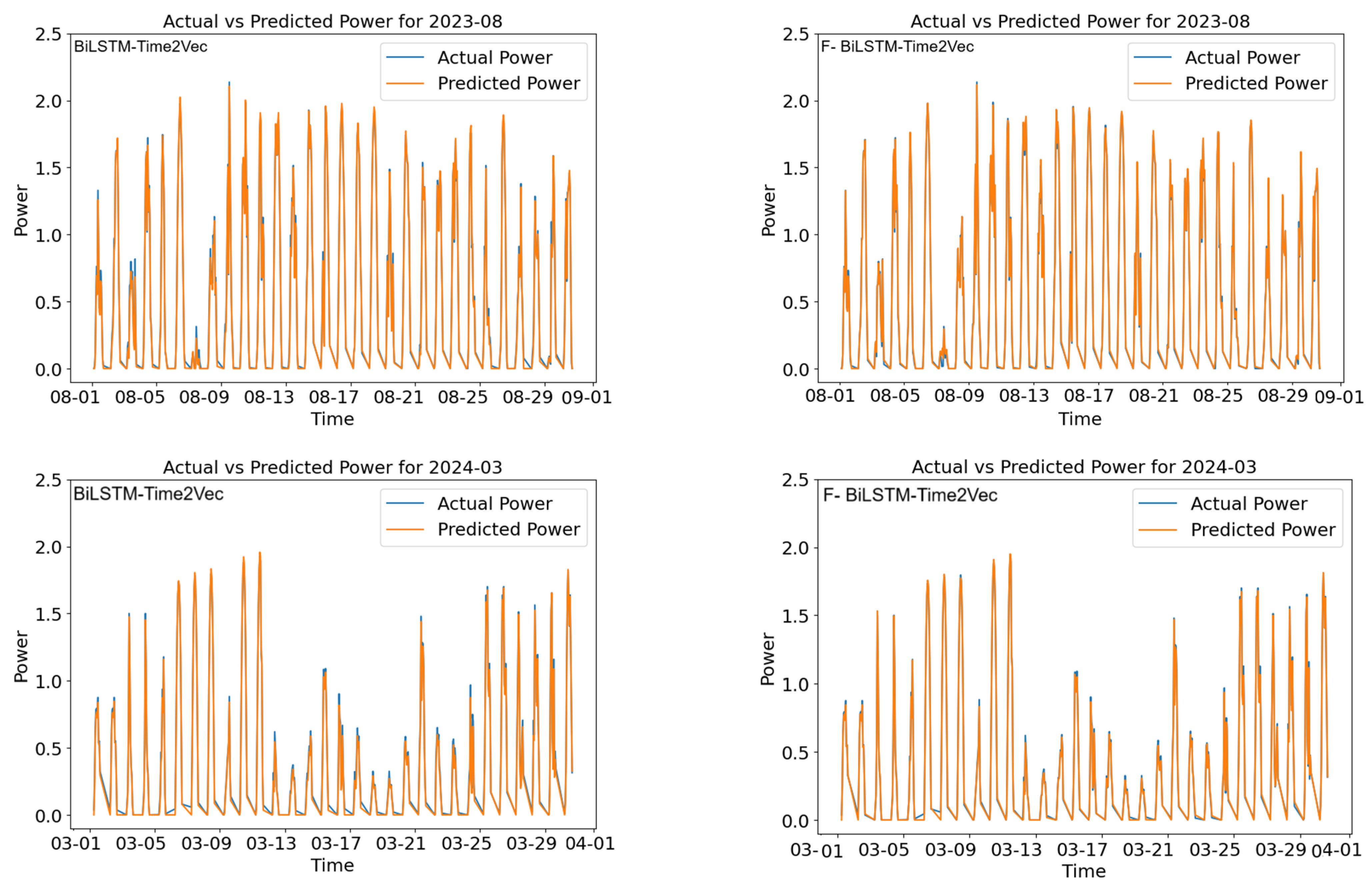
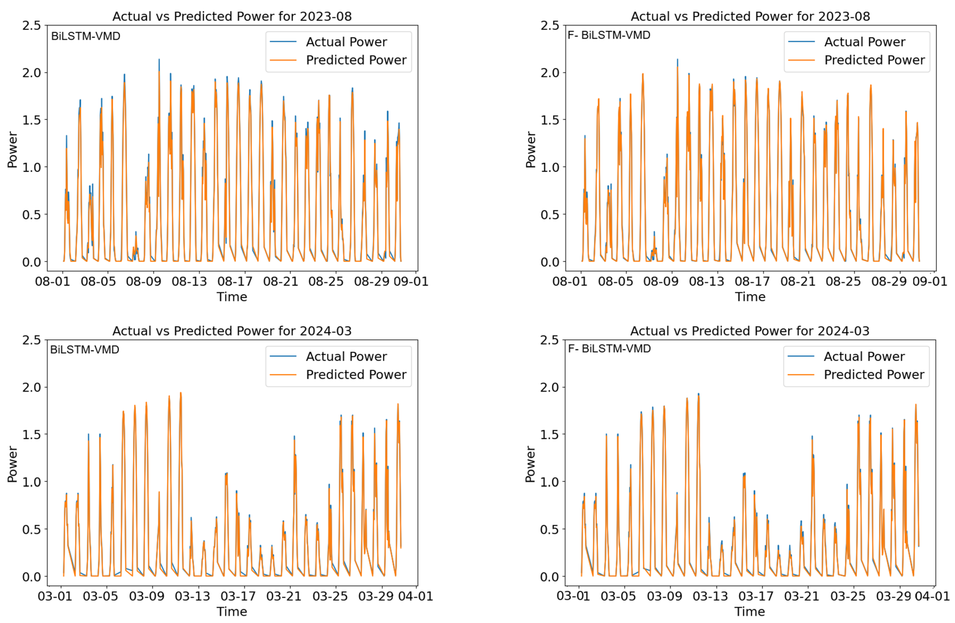
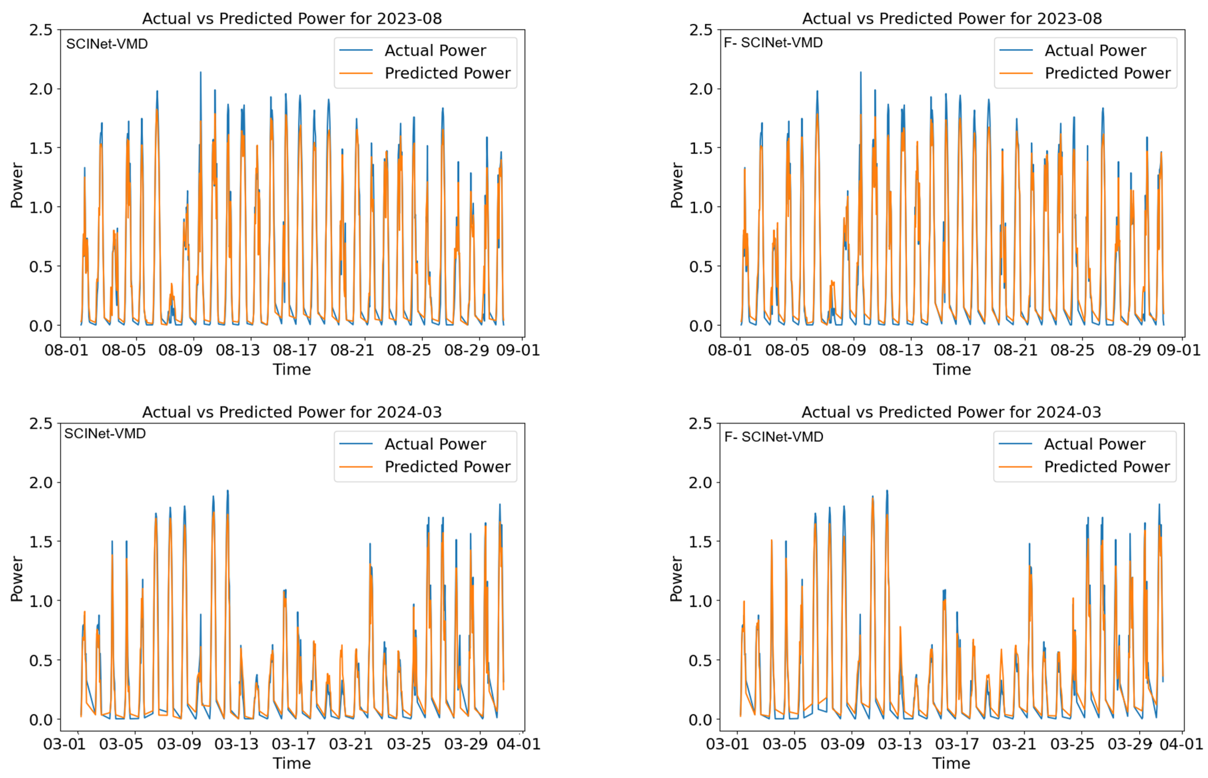
Figure 6, Figure 7, Figure 8 and Figure 9 demonstrate August 2023, from the S&S period, and March 2024, from the F&W period, representing the months when all models achieved their most consistent and generally better performance. This pattern holds for nRMSE and is reflected in these months’ NMAE and WMAE metrics.

5. Discussion

In the experiment, various variations in LSTM and Convolutional Neural Network (CNN) models are applied to forecast energy production in solar power plants. The literature review suggests that LSTM and CNN are highly effective for predicting renewable energy generation. Therefore, these models have been examined in experimental analysis. This study highlights the effectiveness of combining attention-enhanced deep learning models with specialized preprocessing techniques for solar power forecasting in Lithuania’s unique geographical context. By comparing BiLSTM with attention mechanisms and SCINet with self-attention mechanisms, each integrated with either Time2Vec or VMD preprocessing, we provide valuable insights into solar forecasting in high-latitude regions. The four models, BiLSTM-Time2Vec with attention, BiLSTMVMD with attention, SCINet-Time2Vec with self-attention, and SCINet-VMD with self-attention, have distinct strengths. The BiLSTM variants with attention mechanisms excel at capturing sequential patterns, while the SCINet models with self-attention are more effective at modeling long-range dependencies. Including Time2Vec or VMD preprocessing further enhances the models’ ability to capture periodic patterns in the data.
Lithuania’s geographical location (54° N–56° N) presents specific challenges for solar forecasting. Unlike regions with consistent solar radiation or mild seasonal variations, Lithuania experiences significant fluctuations in daylight hours, ranging from 17 h in summer to only 7 h in winter, which is further complicated by the low solar altitude in winter, which reduces solar radiation intensity even during daylight hours. Additionally, the frequent cloud cover and atmospheric instability in the Baltic region make forecasting more complex compared to areas with stable, sunny climates. Our proposed models performed well under these challenging conditions, demonstrating that attention mechanisms combined with Time2Vec or VMD preprocessing effectively address both seasonal patterns and irregular weather variations. By separating the two preprocessing methods, we could assess their contributions to forecasting accuracy. The findings suggest that this approach could improve grid stability and resource allocation. Moreover, the successful application of these models in Lithuania suggests they could also be applied to other high-latitude regions with similar weather patterns. The comparative analysis of the preprocessing techniques (Time2Vec and VMD) offers valuable directions for future research. Combining attention mechanisms, temporal encoding, and signal decomposition is a promising area for advancing solar power forecasting methods. As the field develops, these techniques can contribute to more accurate and reliable solar power predictions, supporting the integration of renewable energy and enhancing sustainability. This study focuses on seasonal patterns in Lithuania. However, the hybrid fuzzy logic and deep learning method can also be applied to other high-latitude regions (50°–60°N), such as northern Europe and Canada, which show similar seasonal variability. Regions with milder seasonal changes may still benefit from the model’s ability to handle uncertainty, although seasonal adaptability is less important in those areas. Initial testing with data from the Baltic states shows prediction accuracy within 5–10% of Lithuania’s results, suggesting the method is transferable. However, applying the model to very different climates, such as equatorial or desert regions, would require adjustments. A significant limitation of this study is the limited access to photovoltaic (PV) data from other regions. Expanding validation to a broader range of climates is an important direction for future research.
Our study and [13] share the same geographical focus in Lithuania but cover different periods (2023–2024 versus 2019- 2020), allowing for a direct comparison of the advancement in forecasting methodologies. While [13] achieved moderate success using LSTM variations (R2 scores between 0.72 and 0.87, with the best performance R2 = 0.927 in August), our hybrid framework combining GT2 Fuzzy logic with advanced neural architectures demonstrates significant improvements. Our FBiLSTM-Time2Vec configuration not only achieved higher accuracy (approximately 99% in favorable seasons) but also exhibited remarkable stability across seasons (spring/summer: nRMSE = 1.188%, NMAE = 0.813%, WMAE = 3.013%; fall/winter: nRMSE = 1.340%, NMAE = 0.807%, WMAE = 22.149%) which represents a substantial improvement over [13]’s reported 0.3% gain from multivariate inputs and addresses their noted winter performance limitations. Integrating GT2-FL with BiLSTM architecture and Time2Vec encoding has effectively addressed the complex seasonal patterns of Lithuania’s maritime-continental climate, suggesting a significant advancement in renewable energy forecasting methodology. These improvements offer promising implications for grid management and energy planning applications while opening new avenues for future regional adaptation and system integration research.
Figure 10 compares model performance using three error metrics: nRMSE, NMAE, and WMAE, with results broken down into spring and summer, fall and winter, and Overall Average. The analysis reveals a significant advantage in models that use General Type 2-Fuzzyfied datasets (indicated by the “F-” prefix) compared to those using typical datasets. The F-models, such as F-SCINet-Time2Vec, F-BiLSTMTime2Vec, F-SCINet-VMD, and F-BiLSTM-VMD, consistently achieve lower error rates across all metrics, demonstrating the effectiveness of fuzzy data preprocessing. This improvement through General Type 2 Fuzzification is particularly evident in F-BiLSTM-Time2Vec, which shows remarkably low error rates in nRMSE and NMAE metrics. The consistent superior performance of F-models across different seasons suggests that General Type 2 Fuzzification provides a more robust approach to handling data uncertainties and variations than the original, non-fuzzified datasets. This pattern indicates that incorporating fuzzy logic in dataset preprocessing can significantly enhance model prediction accuracy.

6. Conclusions

Our study introduces significant advancements in time series forecasting by developing and evaluating hybrid frameworks that combine General Type-2 Fuzzy logic systems with advanced neural architectures. We tested four distinct hybrid frameworks using data from Lithuania (2023–2024). We demonstrated the effectiveness of different architectural combinations in handling complex temporal patterns and seasonal variations. The fuzzified BiLSTM with Time2Vec (F-BiLSTM-Time2Vec) emerged as the most effective configuration, achieving exceptional accuracy with notably low error rates during spring and summer (nRMSE = 1.188%, NMAE = 0.813%, WMAE = 3.013%). Distinctively, the model maintained stable performance even during the challenging fall and winter periods (nRMSE = 1.340%, NMAE = 0.807%, WMAE = 22.149%). This hybrid approach, combining fuzzy logic with BiLSTM architecture and Time2Vec encoding, demonstrates consistently high accuracy levels of around 99% during favorable seasons, providing stability crucial for practical applications in grid management and energy planning. Our analysis reveals several key insights about the relative effectiveness of different components. The BiLSTM-based architectures consistently outperformed SCINet models in handling the complex seasonal patterns of Lithuania’s maritime–continental climate.
While both preprocessing techniques showed promise, Time2Vec encoding proved particularly effective when enhanced with fuzzification, surpassing the moderate effectiveness of VMD preprocessing. Integrating General Type-2 Fuzzy logic significantly improved the model’s ability to handle uncertainties and complex patterns inherent in seasonal data. Our hybrid methodology’s robust performance has important implications for renewable energy forecasting and grid integration. The ability to maintain high accuracy levels, particularly during challenging seasonal transitions, suggests that this approach could significantly improve the reliability of forecasting systems across various applications. This study focuses on Lithuanian conditions; the insights gained provide valuable guidance for developing robust forecasting systems across different geographical contexts. This research opens several promising avenues for future investigation, including adapting these models across various regions, exploring additional preprocessing techniques, and potentially integrating with other forecasting systems. The demonstrated success of combining appropriate architecture choice with temporal encoding and fuzzification suggests that this approach could significantly enhance forecasting accuracy across various domains where reliable prediction is crucial. These findings represent a meaningful step toward developing more accurate and dependable forecasting systems with potential applications that extend well beyond the specific context of this study. In the test set evaluation, F-BiLSTM-Time2Vec maintained superior NMAE (0.834%) and WMAE (3.099%) metrics while showing competitive nRMSE (1.532%) performance. The consistency of F-BiLSTM-Time2Vec across seasons makes it valuable for grid operators to prioritize year-round reliability, though each model offers distinct advantages in different scenarios. Future work should explore geographic generalization and real-time deployment, as the success of both fuzzification and temporal encoding approaches advances robust forecasting in renewable energy applications.

Author Contributions

Conceptualization, N.M.L. and D.N.; methodology, N.M.L. and D.N.; software, N.M.L.; validation, N.M.L., D.N., and G.K.; formal analysis, G.K.; investigation, N.M.L.; resources, D.N. and V.R.; data curation, D.N. and V.R.; writing—original draft preparation, N.M.L.; writing—review and editing, N.M.L., D.N., G.K., and V.R.; visualization, N.M.L. and G.K.; supervision, D.N.; project administration, V.R.; funding acquisition, D.N. and V.R. All authors have read and agreed to the published version of the manuscript.

Funding

This research was funded by a grant (ATE-No. P-LU-24-110) from the Research Council of Lithuania.

Institutional Review Board Statement

Not applicable.

Informed Consent Statement

Not applicable.

Data Availability Statement

The meteorological data used in this study were obtained from the Lithuanian Hydrometeorological Service (LHMT) through their API (https://api.meteo.lt/) (accessed on 5 September 2024).

Acknowledgments

The authors acknowledge the Lithuanian Hydrometeorological Service (LHMT) for providing access to meteorological data through their API. We also thank the Smart Grids and Renewable Energy Laboratory at the Lithuanian Energy Institute for providing computational resources and technical support.

Conflicts of Interest

The authors declare no conflicts of interest. The funders had no role in the study’s design; in the collection, analyses, or interpretation of data; in the writing of the manuscript; or in the decision to publish the results.

Abbreviations

The following abbreviations are used in this manuscript:
AbbreviationFull Form
ADFAugmented Dickey–Fuller
AIArtificial Intelligence
ANNArtificial Neural Network
ANOVAAnalysis of Variance
APIApplication Programming Interface
ARIMAAutoregressive Integrated Moving Average
BiGRUBidirectional Gated Recurrent Unit
BiLSTMBidirectional Long Short-Term Memory
CEEMDANComplete Ensemble Empirical Mode Decomposition with Adaptive Noise
CNNConvolutional Neural Network
CPVConcentrated Photovoltaic
CSPConcentrated Solar Power
DHIDiffuse Horizontal Irradiance
DLDeep Learning
DNNDeep Neural Network
DNIDirect Normal Irradiance
EMDEmpirical Mode Decomposition
EUEuropean Union
F&WFall and Winter
FLFuzzy Logic
FOUFootprint of Uncertainty
GANGenerative Adversarial Network
GHGGreenhouse Gas
GHIGlobal Horizontal Irradiance
GRUGated Recurrent Unit
GT2-FLGeneral Type-2 Fuzzy Logic
IMFIntrinsic Mode Function
KPSSKwiatkowski-Phillips-Schmidt-Shin
LHMTLithuanian Hydrometeorological Service
LSTMLong Short-Term Memory
MAEMean Absolute Error
MAPEMean Absolute Percentage Error
MREMean Relative Error
NARXNon-linear Autoregressive Exogenous
NMAENormalized Mean Absolute Error
nRMSENormalized Root Mean Square Error
PSOParticle Swarm Optimization
PVPhotovoltaic
RERenewable Energy
RMSERoot Mean Square Error
RNNRecurrent Neural Network
S&SSpring and Summer
SCINetSample Convolution and Interactive Neural Network
SVMSupport Vector Machine
T1-FLType-1 Fuzzy Logic
T1-FSType-1 Fuzzy Set
T2-FLType-2 Fuzzy Logic
T2-FSType-2 Fuzzy Set
TCNTemporal Convolutional Network
Time2VecTime to Vector
TWhTerawatt hours
UHDUltra High Definition
VMDVariational Mode Decomposition
WMAEWeighted Mean Absolute Error
WOAWhale Optimization Algorithm

References

  1. Paramati, S.R.; Shahzad, U.; Doğan, B. The role of environmental technology for energy demand and energy efficiency: Evidence from OECD countries. Renew. Sustain. Energy Rev. 2022, 153, 111735. [Google Scholar] [CrossRef]
  2. Paraschiv, L.S.; Paraschiv, S. Contribution of renewable energy (hydro, wind, solar and biomass) to decarbonization and transformation of the electricity generation sector for sustainable development. Energy Rep. 2023, 9, 535–544. [Google Scholar] [CrossRef]
  3. Foley, A.M.; McIlwaine, N.; Morrow, D.J.; Hayes, B.P.; Zehir, M.A.; Mehigan, L.; Papari, B.; Edrington, C.S.; Baran, M. A critical evaluation of grid stability and codes, energy storage and smart loads in power systems with wind generation. Energy 2020, 205, 117671. [Google Scholar] [CrossRef]
  4. Simsek, Y.; Santika, W.G.; Anisuzzaman, M.; Urmee, T.; Bahri, P.A.; Escobar, R. An analysis of additional energy requirement to meet the sustainable development goals. J. Clean. Prod. 2020, 272, 122646. [Google Scholar] [CrossRef]
  5. Eurostat. Renewable Energy Statistics. Available online: https://ec.europa.eu/eurostat/statistics-explained/index.php?title=Renewable_energy_statistics (accessed on 4 July 2025).
  6. Sharma, N.; Sharma, P.; Irwin, D.; Shenoy, P. Predicting solar generation from weather forecasts using machine learning. In Proceedings of the IEEE International Conference on Smart Grid Communications (SmartGridComm), Brussels, Belgium, 17–20 October 2011; pp. 528–533. [Google Scholar] [CrossRef]
  7. Nwagu, C.N.; Ujah, C.O.; Kallon, D.V.; Aigbodion, V.S. Integrating solar and wind energy into the electricity grid for improved power accessibility. Unconv. Resour. 2025, 5, 100129. [Google Scholar] [CrossRef]
  8. Cocco, D.; Migliari, L.; Petrollese, M. A hybrid CSP–CPV system for improving the dispatchability of solar power plants. Energy Convers. Manag. 2016, 114, 312–323. [Google Scholar] [CrossRef]
  9. Rodríguez, F.; Fleetwood, A.; Galarza, A.; Fontán, L. Predicting solar energy generation through artificial neural networks using weather forecasts for microgrid control. Renew. Energy 2018, 126, 855–864. [Google Scholar] [CrossRef]
  10. Moser Baer Solar. Solar PV Monitoring: Maximizing Performance Through Real-Time Analytics. Available online: https://www.moserbaersolar.com/maintenance-and-performance-optimization/solar-pv-monitoring-maximizing-performance-through-real-time-analytics/ (accessed on 4 July 2025).
  11. Rodriguez, J.; Pontt, J.; Correa, P.; Lezana, P.; Cortes, P. Predictive power control of an AC/DC/AC converter. In Proceedings of the 40th IAS Annual Meeting Conference Record of the Industry Applications Conference, Hong Kong, China, 2–6 October 2005; pp. 934–939. [Google Scholar]
  12. Narkutė, V. Forecast of Energy Produced by Solar Power Plants. Ph.D. Thesis, Vilniaus Universitetas, Vilnius, Lithuania, 2022. [Google Scholar]
  13. Mellit, A.; Massi Pavan, A.; Ogliari, E.; Leva, S.; Lughi, V. Advanced methods for photovoltaic output power forecasting: A review. Appl. Sci. 2020, 10, 487. [Google Scholar] [CrossRef]
  14. Sobri, S.; Koohi-Kamali, S.; Rahim, N.A. Solar photovoltaic generation forecasting methods: A review. Energy Convers. Manag. 2018, 156, 459–497. [Google Scholar] [CrossRef]
  15. Kudo, M.; Takeuchi, A.; Nozaki, Y.; Endo, H.; Sumita, J. Forecasting electric power generation in a photovoltaic power system for an energy network. Electr. Eng. Jpn. 2009, 167, 16–23. [Google Scholar] [CrossRef]
  16. Sen, Z. Fuzzy algorithm for estimation of solar irradiation from sunshine duration. Sol. Energy 1998, 63, 39–49. [Google Scholar] [CrossRef]
  17. Gautam, N.K.; Kaushika, N.D. A model for the estimation of global solar radiation using fuzzy random variables. J. Appl. Meteorol. Climatol. 2002, 41, 1267–1276. [Google Scholar] [CrossRef]
  18. Rizwan, M.; Jamil, M.; Kirmani, S.; Kothari, D.P. Fuzzy logic-based modeling and estimation of global solar energy using meteorological parameters. Energy 2014, 70, 685–691. [Google Scholar] [CrossRef]
  19. Nalbant, K.G.; Özdemir, Ş.; Özdemir, Y. Evaluating the campus climate factors using an interval type-2 fuzzy ANP. Sigma J. Eng. Nat. Sci. 2024, 42, 89–98. [Google Scholar] [CrossRef]
  20. Mendel, J.M.; John, R.B. Type 2-Fuzzy sets made simple. IEEE Trans. Fuzzy Syst. 2002, 10, 117–127. [Google Scholar] [CrossRef]
  21. Hinton, G.E.; Osindero, S.; Teh, Y. A fast learning algorithm for deep belief nets. Neural Comput. 2006, 18, 1527–1554. [Google Scholar] [CrossRef]
  22. Jlidi, M.; Hamidi, F.; Barambones, O.; Abbassi, R.; Jerbi, H.; Aoun, M.; Karami-Mollaee, A. An artificial neural network for solar energy prediction and control using Jaya-SMC. Electronics 2023, 12, 592. [Google Scholar] [CrossRef]
  23. Zhidan, L.; Wei, G.; Qingfu, L.; Zhengjun, Z. A hybrid model for financial time-series forecasting based on mixed methodologies. Expert Syst. 2021, 38, e12633. [Google Scholar]
  24. Ni, Z.; Zhang, C.; Karlsson, M.; Gong, S. A study of deep learning-based multi-horizon building energy forecasting. Energy Build. 2024, 303, 113810. [Google Scholar] [CrossRef]
  25. Bai, S.; Kolter, J.Z.; Koltun, V. An empirical evaluation of generic convolutional and recurrent networks for sequence modeling. arXiv 2018, arXiv:1803.01271. [Google Scholar] [CrossRef]
  26. Li, Y.; Song, L.; Zhang, S.; Kraus, L.; Adcox, T.; Willardson, R.; Komandur, A.; Lu, N. A TCN-based hybrid forecasting framework for hours-ahead utility-scale PV forecasting. IEEE Trans. Smart Grid 2023, 14, 4073–4085. [Google Scholar] [CrossRef]
  27. Kong, X.; Du, X.; Xu, Z.; Xue, G. Predicting solar radiation for space heating with thermal storage system based on temporal convolutional network-attention model. Appl. Therm. Eng. 2023, 219, 119574. [Google Scholar] [CrossRef]
  28. Liu, M.; Qin, H.; Cao, R.; Deng, S. Short-term load forecasting based on improved TCN and DenseNet. IEEE Access 2022, 10, 115945–115957. [Google Scholar] [CrossRef]
  29. Limouni, T.; Yaagoubi, R.; Bouziane, K.; Guissi, K.; Baali, E.H. Accurate one step and multistep forecasting of very short-term PV power using LSTM-TCN model. Renew. Energy 2023, 205, 1010–1024. [Google Scholar]
  30. Zhao, Y.; Peng, X.; Tu, T.; Li, Z.; Yan, P.; Li, C. WOA-VMD-SCINet: Hybrid model for accurate prediction of ultra-short-term Photovoltaic generation power considering seasonal variations. Energy Rep. 2024, 12, 3470–3487. [Google Scholar] [CrossRef]
  31. Huang, X.; Li, Q.; Tai, Y.; Chen, Z.; Liu, J.; Shi, J.; Liu, W. Time series forecasting for hourly photovoltaic power using conditional generative adversarial network and Bi-LSTM. Energy 2022, 246, 123403. [Google Scholar] [CrossRef]
  32. Zhang, C.; Peng, T.; Nazir, M.S. A novel integrated photovoltaic power forecasting model based on variational mode decomposition and CNN-BiGRU considering meteorological variables. Electr. Power Syst. Res. 2022, 213, 108796. [Google Scholar] [CrossRef]
  33. Trong, T.N.; Son, H.V.X.; Dinh, H.D.; Takano, H.; Duc, T.N. Short-term PV power forecast using hybrid deep learning model and Variational Mode Decomposition. Energy Rep. 2023, 9, 712–717. [Google Scholar] [CrossRef]
  34. Wang, X.; Ma, W. A hybrid deep learning model with an optimal strategy based on improved VMD and transformer for short-term photovoltaic power forecasting. Energy 2024, 295, 131071. [Google Scholar] [CrossRef]
  35. Peng, S.; Zhu, J.; Wu, T.; Yuan, C.; Cang, J.; Zhang, K.; Pecht, M. Prediction of wind and PV power by fusing the multi-stage feature extraction and a PSO-BiLSTM model. Energy 2024, 298, 131345. [Google Scholar] [CrossRef]
  36. Voyant, C.; Notton, G.; Kalogirou, S.; Nivet, M.L.; Paoli, C.; Motte, F.; Fouilloy, A. Machine learning methods for solar radiation forecasting: A review. Renew. Energy 2017, 105, 569–582. [Google Scholar] [CrossRef]
  37. Chaturvedi, D.K.; Isha, I. Solar power forecasting: A review. Int. J. Comput. Appl. 2016, 140, 28–50. [Google Scholar] [CrossRef]
  38. Rana, M.; Rahman, A. Multiple steps ahead solar photovoltaic power forecasting based on univariate machine learning models and data re-sampling. Sustain. Energy Grids Netw. 2020, 21, 100286. [Google Scholar] [CrossRef]
  39. Wang, K.; Qi, X.; Liu, H. A comparison of day-ahead photovoltaic power forecasting models based on deep learning neural network. Appl. Energy 2019, 251, 113315. [Google Scholar] [CrossRef]
  40. Gao, M.; Li, J.; Hong, F.; Long, D. Day-ahead power forecasting in a large-scale photovoltaic plant based on weather classification using LSTM. Energy 2019, 187, 115838. [Google Scholar] [CrossRef]
  41. Qing, X.; Niu, Y. Hourly day-ahead solar irradiance prediction using weather forecasts by LSTM. Energy 2018, 148, 461–468. [Google Scholar] [CrossRef]
  42. Cabello-López, T.; Carranza-García, M.; Riquelme, J.C.; García-Gutiérrez, J. Forecasting solar energy production in Spain: A comparison of univariate and multivariate models at the national level. Appl. Energy 2023, 350, 121645. [Google Scholar] [CrossRef]
  43. Gao, B.; Huang, X.; Shi, J.; Tai, Y.; Zhang, J. Hourly forecasting of solar irradiance based on CEEMDAN and multi-strategy CNN-LSTM neural networks. Renew. Energy 2020, 162, 1665–1683. [Google Scholar] [CrossRef]
  44. Liu, M.; Zeng, A.; Chen, M.; Xu, Z.; Lai, Q.; Ma, L.; Xu, Q. Scinet: Time series modeling and forecasting with sample convolution and interaction. Adv. Neural Inf. Process. Syst. 2022, 35, 5816–5828. [Google Scholar]
  45. Li, F.F.; Wang, S.Y.; Wei, J.H. Long term rolling prediction model for solar radiation combining empirical mode decomposition (EMD) and artificial neural network (ANN) techniques. J. Renew. Sustain. Energy 2018, 10, 1. [Google Scholar] [CrossRef]
  46. Lanbaran, N.M.; Celik, E.; Yigider, M. Evaluation of investment opportunities with interval-valued fuzzy TOPSIS method. Appl. Math. Nonlinear Sci. 2020, 5, 461–474. [Google Scholar] [CrossRef]
  47. Melin, P.; Castillo, O. A review on Type 2-Fuzzy logic applications in clustering, classification and pattern recognition. Appl. Soft Comput. 2014, 21, 568–577. [Google Scholar] [CrossRef]
  48. Mittal, K.; Jain, A.; Vaisla, K.S.; Castillo, O.; Kacprzyk, J. A comprehensive review on type 2 fuzzy logic applications: Past, present and future. Eng. Appl. Artif. Intell. 2020, 95, 103916. [Google Scholar] [CrossRef]
  49. Juang, C.-F.; Huang, R.-B.; Lin, Y.-Y. A recurrent self-evolving interval Type 2-Fuzzy neural network for dynamic system processing. IEEE Trans. Fuzzy Syst. 2009, 17, 1092–1105. [Google Scholar] [CrossRef]
  50. Geng, D.; Wang, B.; Gao, Q. A hybrid photovoltaic/wind power prediction model based on Time2Vec, WDCNN and BiLSTM. Energy Convers. Manag. 2023, 291, 117342. [Google Scholar] [CrossRef]
  51. Zosso, D.; Dragomiretskiy, K.; Bertozzi, A.L.; Weiss, P.S. Two-dimensional compact variational mode decomposition: Spatially compact and spectrally sparse image decomposition and segmentation. J. Math. Imaging Vis. 2017, 58, 294–320. [Google Scholar] [CrossRef]
  52. Guermoui, M.; Fezzani, A.; Mohamed, Z.; Rabehi, A.; Ferkous, K.; Bailek, N.; Ghoneim, S.S.M. An analysis of case studies for advancing photovoltaic power forecasting through multi-scale fusion techniques. Sci. Rep. 2024, 14, 6653. [Google Scholar] [CrossRef] [PubMed]
  53. Efimov, V.M.; Reznik, A.L.; Bondarenko, Y.V. Increasing the sine-cosine transformation accuracy in signal approximation and interpolation. Optoelectron. Instrum. Data Process. 2008, 44, 218–227. [Google Scholar] [CrossRef]
  54. Niu, Z.; Zhong, G.; Yu, H. A review on the attention mechanism of deep learning. Neurocomputing 2021, 452, 48–62. [Google Scholar] [CrossRef]
  55. Lin, J.; Ma, J.; Zhu, J.; Cui, Y. Short-term load forecasting based on LSTM networks considering attention mechanism. Int. J. Electr. Power Energy Syst. 2022, 137, 107818. [Google Scholar] [CrossRef]
  56. Yang, M.; Wang, J. Adaptability of financial time series prediction based on BiLSTM. Procedia Comput. Sci. 2022, 199, 18–25. [Google Scholar] [CrossRef]
  57. Parri, S.; Teeparthi, K. VMD-SCINet: A hybrid model for improved wind speed forecasting. Earth Sci. Inform. 2024, 17, 329–350. [Google Scholar] [CrossRef]
  58. Dong, P.; Zuo, Y.; Chen, L.; Li, S.; Zhang, L. VSNT: Adaptive Network Traffic Forecasting via VMD and Deep Learning with SCI-Block and Attention Mechanism. In Proceedings of the 2023 IEEE International Conference on Parallel and Distributed Processing with Applications, Big Data and Cloud Computing, Sustainable Computing and Communications, Social Computing and Networks (ISPA/BDCloud/SocialCom/SustainCom), Haikou, China, 21–23 December 2023; pp. 104–109. [Google Scholar]
  59. Leva, S.; Dolara, A.; Grimaccia, F.; Mussetta, M.; Ogliari, E. Analysis and validation of 24 hours ahead neural network forecasting of photovoltaic output power. Math. Comput. Simul. 2017, 131, 88–100. [Google Scholar] [CrossRef]
  60. Arltová, M.; Fedorová, D. Selection of Unit Root Test on the Basis of Length of the Time Series and Value of AR (1) Parameter. Stat. Stat. Econ. J. 2016, 96, 4–17. [Google Scholar]
  61. Musbah, H.; Aly, H.H.; Little, T.A. A proposed novel adaptive DC technique for non-stationary data removal. Heliyon 2023, 9, 3. [Google Scholar] [CrossRef] [PubMed]
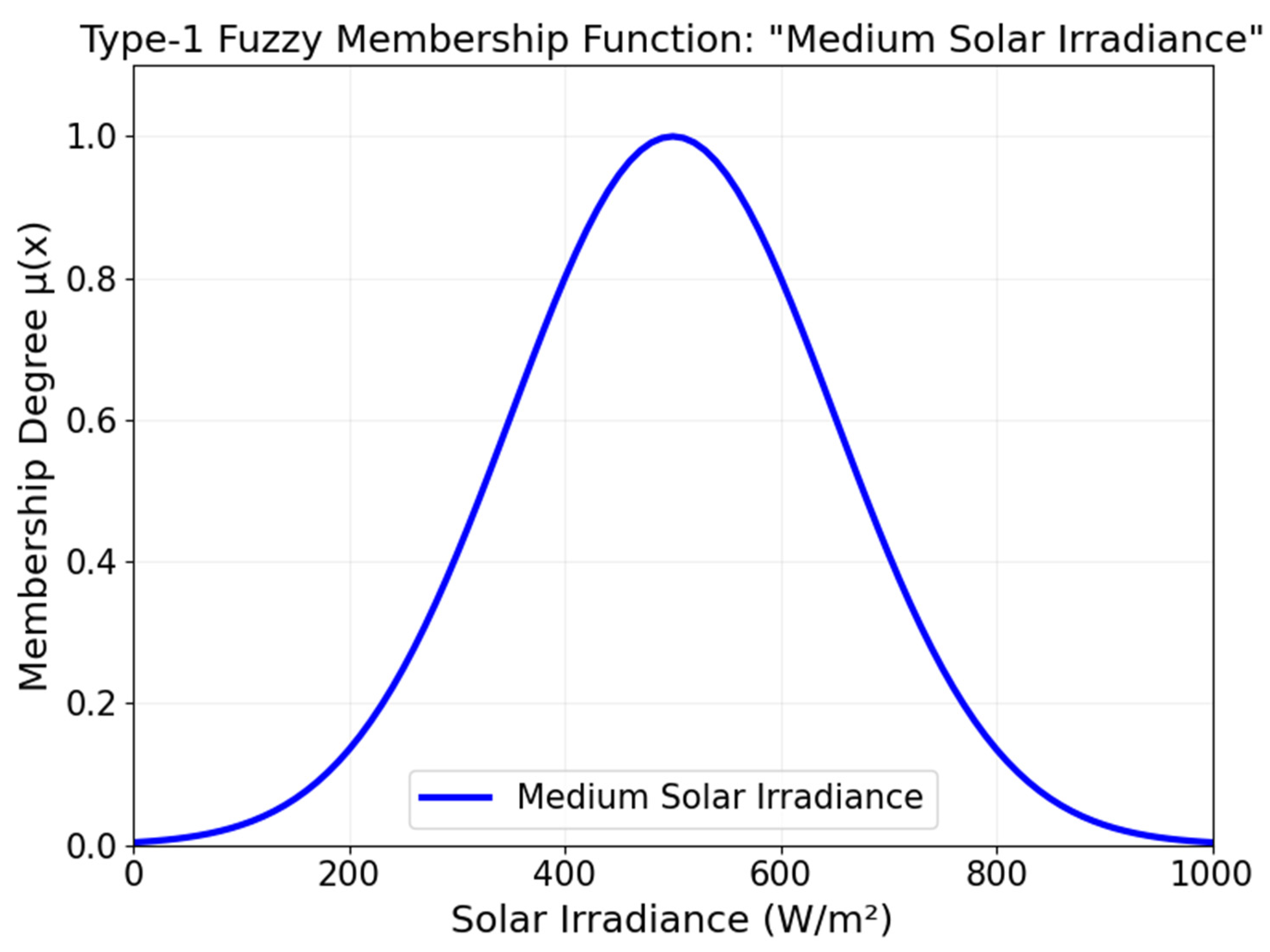
Figure 1. Type-1 Fuzzy Gaussian membership function developed by the authors.
Applsci 15 09672 g001
Figure 2. General Type 2- Fuzzy membership function, developed by authors.
Applsci 15 09672 g002
Figure 3. Data preprocessing methodology flowchart developed by the authors.
Applsci 15 09672 g003
Figure 4. Correlation Between Meteorological Variables and PV Power Output, developed by the authors.
Applsci 15 09672 g004
Figure 5. Overview of the hybrid forecasting methodology showing data preprocessing, model architecture, and evaluation framework.
Applsci 15 09672 g005
Figure 6. Actual versus predicted solar power generation for BiLSTM-Time2Vec and F-BiLSTM models during S&S and F&W periods.
Applsci 15 09672 g006
Figure 7. Actual versus predicted solar power generation for SCINet-Time2Vec and F-SCINet-Time2Vec models during S&S and F&W periods.
Applsci 15 09672 g007aApplsci 15 09672 g007b
Figure 8. Actual versus predicted solar power generation for BiLSTM-VMD and F-BiLSTM-VMD models during S&S and F&W periods.
Applsci 15 09672 g008
Figure 9. Actual versus predicted solar power generation for SCINet-VMD and F-SCINet-VMD models during S&S and F&W periods.
Applsci 15 09672 g009
Figure 10. Comparative performance analysis of all model variants across nRMSE, NMAE, and WMAE metrics for spring/summer, fall/winter, and overall periods.
Applsci 15 09672 g010
Table 1. Comparative Overview of Solar Forecasting Approaches.
Approach CategoryKey MethodsLimitationsBest PerformanceReference
Statistical Models ARIMA, SVM, Random Forest Limited handling of non-linear patterns15% MRE (Random Forest), 17.70% MAPE (ARIMA)[36,37,38]
Classical Neural Networks ANN, CNN, DNN Difficulty with temporal dependenciesR2 = 0.93 (ANN monthly), R = 0.92 (NARX NN)[22,39]
Recurrent Architectures LSTM, BiLSTM, GRU Computational complexity, gradient issues5% nRMSE (LSTM), 7% nMAE (LSTM), 8% nMAE (GRU)[24,40,41]
Hybrid Deep Learning CNN-LSTM, TCN-DenseNet High computational requirements23.38% MAPE reduction (TCN-DN), 38.49% error rate (CEEM-CNN-LSTM)[28,42,43]
Advanced Architectures SCINet, Transformer Complex hyperparameter tuning13.7% MAE (VMD-Transformer), 0.619–1.149 kW RMSE (WOA-VMD-SCINet)[33,34,44]
Signal Processing VMD, EMD, CEEMDAN Preprocessing complexity93.0% correlation (monthly), 69.8% correlation (daily), 29.05% RMSE, 4.157 RMSE[32,43,45]
Note: Lower values indicate better performance for error metrics (MAPE, MRE, nRMSE, nMAE, RMSE, MAE, Error Rate). Higher values indicate better performance for accuracy metrics (R2, correlation coefficients).
Table 2. Optimized hyperparameters used across all model variants.
Parameter CategoryParameterValue
Data ConfigurationLook Back Window24
Forecast Horizon1
Training Period1 January 2023 08:00–5 August 2023 18:00
Validation Period6 August 2023 03:00–15 June 2024 19:00
Testing Period16 June 2024 02:00–31 August 2024 17:00
Training ParametersBatch Size42
Learning Rate1.00 × 10−3
Weight Decay1.00 × 10−5
Loss Function
Epochs
0.4MSE + 0.3MAE + 0.3Huber
100
ArchitectureMain Units[512, 256, 128, 64]
Time2Vec Modelskernel_size = 64, Dropout: LSTM 0.2, Dense 0.1
VMD ModelsK = 3 modes, Dropout: LSTM 0.2, Dense 0.1
Table 3. Performance Metrics Comparison of BiLSTM Variants.
DateF- BiLSTM-Time2VecBiLSTM-Time2VecF-BiLSTM-VMDBiLSTM-VMD
nRMSENMAEWMAEnRMSENMAEWMAEnRMSENMAEWMAEnRMSENMAEWMAE
S&S
2023-041.09950.74673.28001.20820.84573.71491.20120.81103.56231.95091.33225.8516
2023-051.35510.94532.74611.23520.86062.50021.13210.77852.26152.10121.51184.3918
2023-061.19480.83752.86341.36270.93623.20061.21640.82072.80611.96191.36924.6813
2023-071.15740.81702.87591.59741.13874.00821.29510.92153.24381.91521.35194.7586
2023-080.97190.68162.66131.67101.16004.52911.58711.09004.25572.13161.51955.9327
2023-091.09870.74322.40832.20941.63475.29751.68991.15653.74772.92582.14956.9659
2024-041.26970.87144.51411.68601.21716.30501.54771.07485.56772.38971.69878.7997
2024-051.19120.82332.53461.26580.88032.71011.17640.80292.47192.10611.50924.6463
2024-061.15140.78423.06961.48261.01343.96701.34840.90173.52971.95051.33895.2409
2024-071.60300.97063.75292.00551.22174.72401.51101.04234.03022.29311.54865.9878
2024-080.97200.71692.43851.56321.09993.74121.50141.06463.62102.10731.51565.1549
F&W
2023-010.94100.499928.41221.30340.708640.27261.23420.706940.17701.56450.886550.3838
2023-021.08670.71838.03961.71221.147512.84301.41190.985511.03052.01101.383615.4861
2023-030.89350.61543.16451.61531.21306.23791.19760.84374.33862.02561.43617.3851
2023-102.13311.409210.70942.76251.852214.07672.72391.746013.26943.77122.464818.7321
2023-112.70271.721136.17143.09771.935140.66893.89452.319848.75394.45112.648755.6667
2023-121.58200.638787.40592.32550.9315127.48461.79990.704996.46371.87400.722698.8857
2024-010.61960.254212.30431.17010.483323.39380.95790.409019.79901.28480.537626.0215
2024-021.05370.70189.57341.87251.258317.16501.68271.140715.56082.21311.526220.8197
2024-031.04470.70873.56221.51491.10405.54931.31680.91994.62402.15071.55787.8308
Averages
Ave of S&S1.18770.81253.01321.57151.09174.06341.38240.95133.55432.16671.53145.6738
Ave of F&W1.33970.807522.14921.93051.181531.96581.80221.086328.22412.37181.462733.4679
Entire Ave1.25610.810311.62441.73311.132116.61951.57131.012014.65572.25901.500518.1812
Test Set1.53200.83403.09902.69731.33924.97801.7241.06303.95202.99621.44703.625
Table 4. Performance Metrics Comparison of SCINet Variants.
DateF-SCINet-Time2VecSCINet-Time2VecF-SCINet-VMDSCINet-VMD
nRMSENMAEWMAEnRMSENMAEWMAEnRMSENMAEWMAEnRMSENMAE WMAE
S&S
2023-044.18632.487310.92553.70302.21689.73754.55083.222914.15684.35333.190014.0123
2023-054.99303.29689.57774.14482.71577.88935.07333.502310.17455.08243.618810.5131
2023-064.48512.89129.88483.89732.48078.48144.23672.82359.65334.59133.019910.3247
2023-074.34232.80229.86383.62882.36158.31253.82292.63159.26304.64753.140511.0545
2023-084.00352.573010.04553.72682.41049.41094.82803.302012.89185.14433.478313.5801
2023-093.44532.21147.16633.11222.02436.55996.77374.450514.42236.48184.332114.0388
2024-043.57222.174111.26253.51962.220011.50015.70423.796519.66685.57773.696719.1496
2024-054.96383.15749.72074.57642.78098.56175.23253.518310.83175.01543.418110.5233
2024-064.14572.573310.07313.78122.33789.15124.62283.023911.83674.72793.087412.0855
2024-074.53982.746410.61944.30672.54609.84486.16783.936615.22195.88503.949515.2718
2024-083.80822.45278.34243.43402.19477.46485.27563.514511.95395.77363.908213.2930
F&W
2023-011.44821.151265.42671.56711.226769.71881.14670.873849.66181.75741.343476.3508
2023-022.40271.347815.08572.39431.476016.51992.30861.597617.88142.78942.055523.0055
2023-033.53342.091610.75603.16461.89189.72833.50822.403712.36093.82492.671913.7398
2023-1014.68238.565865.098816.59729.363971.164610.63156.467449.15109.93146.167246.8697
2023-118.01004.135086.90278.96924.460893.75115.81133.647676.66125.59103.709877.9664
2023-121.91300.7307100.00001.91300.7307100.00004.64343.3954464.67115.89904.4411607.7771
2024-012.76052.0812100.73872.97072.1891105.96532.94371.960494.89393.55642.4776119.9293
2024-022.67171.580221.55732.45591.440719.65383.96452.252130.72304.09162.643436.0611
2024-033.95562.531312.72433.69992.381011.96864.72693.185016.01014.50843.112015.6431
Averages
Ave of S&S4.22592.66969.77113.80282.38998.81045.11713.429312.73395.20733.530913.0770
Ave of F&W4.59752.690553.14344.85912.795655.38564.40942.864890.22384.66113.1802113.0381
Entire Ave4.39312.679029.28864.27812.572529.76924.79873.175347.60444.96153.373158.0595
Test Set4.53102.63319.78624.43002.54329.45015.58603.626313.47515.83343.750413.9360
Disclaimer/Publisher’s Note: The statements, opinions and data contained in all publications are solely those of the individual author(s) and contributor(s) and not of MDPI and/or the editor(s). MDPI and/or the editor(s) disclaim responsibility for any injury to people or property resulting from any ideas, methods, instructions or products referred to in the content.