Efficient Target Assignment via Binarized SHP Path Planning and Plasticity-Aware RL in Urban Adversarial Scenarios

Abstract

Accurate and feasible target assignment in an urban environment without road networks remains challenging. Existing methods exhibit critical limitations: computational inefficiency preventing real-time decision-making requirements and poor cross-scenario generalization, yielding task-specific policies that lack adaptability. To achieve efficient target assignment in urban adversarial scenarios, we propose an efficient traversable path generation method requiring only binarized images, along with four key constraint models serving as optimization objectives. Moreover, we model this optimization problem as a Markov decision process (MDP) and introduce the generalization sequential proximal policy optimization (GSPPO) algorithm within the reinforcement learning (RL) framework. Specifically, GSPPO integrates an exploration history representation module (EHR) and a neuron-specific plasticity enhancement module (NPE). EHR incorporates exploration history into the policy learning loop, which significantly improves learning efficiency. To mitigate the plasticity loss in neural networks, we propose an NPE module, which boosts the model’s representational capability and generalization across diverse tasks. Experiments demonstrate that our approach reduces planning time by four orders of magnitude compared to the online planning method. Against the benchmark algorithm, it achieves 94.16% higher convergence performance, 33.54% shorter assignment path length, 51.96% lower threat value, and 40.71% faster total time. Our approach supports real-time military reconnaissance and will also facilitate rescue operations in complex cities.

1. Introduction

Accelerating urbanization makes military operations in dense urban environments increasingly pivotal [1]. This raises demand for accurate and efficient target assignment in such settings. For target assignment, precise road network information is essential. However, obtaining accurate road network intelligence remains fundamentally challenging [2]. This constraint requires extracting traversable paths from limited situational inputs—especially unmanned aerial vehicle (UAV) reconnaissance imagery. Such path generation forms the critical foundation for real-time target assignment. Here, we focus on urban adversarial target assignment—defined as military engagements that force our units against enemy targets in complex urban environments. Specifically, this is a weapon–target assignment (WTA) variant that optimizes unit distribution (e.g., UGVs) against enemy targets [3].

Target assignment is an NP-hard problem. Its decision space grows exponentially with problem scale—specifically with the number of units and targets [4]. Consequently, solution real-time performance, accuracy, and effectiveness directly impact mission outcomes. These factors determine optimal results in adversarial operations. Current research employs two main algorithmic approaches: traditional exact algorithms based on mixed integer linear programming (MILP) and heuristic algorithms [5].

Traditional exact algorithms mainly address small-scale problems. They often require simplified structural assumptions. Target assignment is typically formulated as an MILP problem [6]. Solution methods include the Hungarian algorithm [7], branch-and-bound algorithm [8,9], and Lagrangian relaxation [10], which rely on classical solvers like Gurobi. However, they do not directly solve the original nonlinear objective function. When the problem size increases, online computation time scales exponentially. This makes it hard to meet strict real-time requirements in practical decision-making. Thus, exact algorithms face scalability limits. Their use is largely restricted to problems with low real-time demands and simple constraints.

Human decision preferences and weapon–target interaction knowledge can be encoded as rules. These rules help construct optimal solutions. Rule-based heuristic algorithms apply such rules during solution construction and search. This enables rapid generation of feasible assignments. Representative methods include genetic algorithms (GAs) [11], particle swarm optimization (PSO) [12], and ant colony optimization (ACO) [13]. However, these algorithms heavily depend on scenario-specific conditions and domain knowledge. They frequently converge to local optima [14]. Although optimization accuracy improves, convergence speed remains limited. Consequently, such algorithms show poor generalization capabilities in high-dimensional real-world problems.

Reinforcement learning (RL) has achieved remarkable breakthroughs in various domains recently [15]. Combinatorial optimization involves selecting optimal variables from discrete decision spaces. This process resembles RL’s action selection mechanism. The offline-to-online paradigm of RL enables real-time combinatorial optimization solutions. Consequently, RL techniques show strong potential for classical combinatorial optimization problems. Traditional methods include value-based algorithms for simplified single-target weapon scenarios [16] and actor-critic algorithms for cooperative target assignment problems [5,17].

However, conventional RL algorithms face four critical limitations in urban adversarial target assignment [18]. First, most methods optimize single tasks, lacking adaptability to diverse mission scenarios. Second, grid-validated algorithms fail in realistic cities with irregular structures [19]. Moreover, traditional approaches ignore the impact of historical decisions on current choices, resulting in low learning efficiency. Furthermore, continual learning gradually reduces neural network adaptability for new tasks—termed plasticity loss. This severely compromises cross-scenario generalization [20].

To overcome these limitations, this paper presents an integrated framework for target assignment in urban adversarial scenarios without road networks. Our solution spans traversable path construction to autonomous assignment scheme generation, enabling efficient real-time planning using only binarized shapefile (SHP) data. The main contributions of this paper are summarized as follows:

• We propose an integrated framework for urban adversarial target assignment without road networks. It generates traversable paths from binarized SHP data and solves assignment via the novel GSPPO algorithm within an MDP formulation.
• We design an EHR module that fully utilizes historical information by integrating environmental interaction trajectories into the policy learning loop, which enhances learning efficiency.
• We develop an NPE module that dynamically recalibrates network parameters during training. It optimizes policy updates while mitigating plasticity loss, which improves the network’s generalization across diverse tasks.
• We validate GSPPO’s effectiveness for urban adversarial target assignment through comprehensive experiments. Results show that GSPPO maintains high decision quality while significantly improving computational efficiency. These capabilities indicate strong practicality for real-time scenarios.

2. Related Work

Urban adversarial target assignment studies the optimal allocation of our units against enemy targets to maximize mission effectiveness. Current research mainly focuses on two aspects: model formulation and algorithm design. Based on problem scale and real-time requirements, existing approaches can be categorized into three major classes: exact algorithms, heuristic algorithms, and RL algorithms. These categories show distinct features in computational complexity, scalability, and real-time performance.

2.1. Exact Algorithms

Exact algorithms seek optimal solutions through mathematical programming frameworks, but due to computational complexity, they are typically only applicable to small-scale problems. Branch-and-bound is a mainstream exact method for solving the WTA problem. Cha et al. [21] proposed a branch-and-bound algorithm for artillery fire scheduling, capable of obtaining optimal solutions for small-scale instances within a reasonable computation time. Kline et al. [22] further introduced a hybrid depth-first search strategy to address nonlinear integer programming formulations of the WTA problem. Lu et al. [23] modeled the WTA problem as a 0–1 integer linear program and improved search efficiency in the solution space by combining branch-and-bound with column generation techniques. Ahner et al. [24] proposed an adaptive dynamic programming approach that integrates concave adaptive value estimation (CAVE) with the max-margin reward (MMR) algorithm, validating solution optimality through a post-decision dynamic programming formulation. Dynamic programming has also been applied to small-scale two-stage WTA problems; however, its practical applicability is limited by the curse of dimensionality [24].

2.2. Heuristic Algorithms

To address larger-scale or more complex WTA problems, researchers have proposed various heuristic algorithms that strike a balance between solution quality and computational efficiency. Rule-based heuristic methods generate feasible solutions rapidly by embedding domain-specific knowledge. Xin et al. [25,26] introduced a virtual permutation-based tabu search approach and a constructive heuristic algorithm, respectively, both of which significantly improved the efficiency of solving medium-scale WTA instances. Chang et al. [27] combined rule-driven population initialization with an improved artificial bee colony algorithm to effectively solve medium-scale WTA problems. Zhang et al. [28] proposed a heuristic algorithm based on statistical marginal reward (HA-SMR), which demonstrated effectiveness in asset-based WTA scenarios. Multi-objective optimization approaches enhance solution diversity by balancing damage probability and resource cost. Yan et al. [29] developed an improved multi-objective particle swarm optimization (MOPSO) algorithm that generates a solution set superior to the general Pareto front by dynamically adjusting learning factors and inertia weights. However, heuristic algorithms are generally unable to guarantee global optimality and exhibit high sensitivity to parameter configurations [27].

2.3. RL Algorithms

In recent years, RL has been introduced into the domain of WTA due to its advantages in dynamic decision-making. RL methods directly learn assignment policies through state-action modeling. Luo et al. [30] proposed an RL-based framework for solving WTA problems, which outperformed traditional heuristic approaches in both solution quality and computational efficiency. Wang et al. [31] integrated deep Q-networks (DQN) with an improved multi-objective artificial bee colony (MOABC) algorithm, enhancing system cumulative reward while reducing time overhead through a hybrid strategy. Multi-objective RL methods further optimize multiple conflicting objectives simultaneously. Zou et al. [32] combined DQN with adaptive mutation and greedy crossover operators, proposing a multi-objective evolutionary algorithm (MOEA) that significantly improved both the convergence and diversity of solutions. Ding et al. [33] designed a distributed PPO algorithm incorporating threat assessment and a dynamic attention mechanism, enabling adaptability to a complex battlefield environment through a hierarchical decision-making framework. LSTM-PPO [18] hybrids capture temporal dependencies in sequential tasks, yet struggle with plasticity loss during task shifts. Curriculum RL (CRL) frameworks employ phased task progression to reduce negative transfer but increase hyperparameter sensitivity. For specific solution methods and their corresponding characteristics and limitations, please refer to

Table 1. Characteristics and limitations of various WTA algorithms.

Algorithms	Existing Approaches	Characteristics	Limitations
Exact Algorithms	Hungarian, branch-and-bound, Lagrangian relaxation, and so on	Optimal	Inefficient
Heuristic Algorithms	GA, MOPSO, ACO, HA-SMR, and so on	Practical	Suboptimal
RL algorithms	DQN, distributed PPO, and so on	Fast solution speed	Weak generalization

.

Our review reveals that traditional WTA frameworks still face critical limitations in urban adversarial scenarios. They inadequately handle assignment mechanisms under complex constraints, especially regarding real-time applicability. Theoretical and methodological innovations remain urgently needed to address complex urban challenges.

To address these gaps, we propose a comprehensive modeling framework for urban adversarial target assignment. Our solution leverages RL foundations. Specifically, it integrates historical interaction trajectories into the learning loop during decision-making. Moreover, it balances adaptability to new strategies with stability of historical policies across diverse scenarios. Experiments verify its ability to generate high-quality solutions efficiently, under real-time constraints, outperforming benchmarks in adaptability metrics.

3. Preliminaries

3.1. MDP

RL achieves decision optimization through interactive learning between the agent and the environment [34]. Within the standard framework of the MDP, RL can be formulated as $M=〈S,A,P,R,\gamma 〉$. Here, $S$ denotes the state space, $A$ denotes the action space, $P(s_{t+1}|s_t,a_t)$ stands for transition dynamics, $r=R(s,a)$ denotes the reward function, and $\gamma \in \left[0,1\right]$ represents the reward discount factor. For any $s\in S$ and action $a\in A$, the value of action $a$ under state $s$ is given by the action-value function $Q^{\pi }(s,a)=\mathbb{E}[{\displaystyle {\sum }_{t=0}^{\infty }{\gamma }^{t}R(s_t,a_t)}]$. The objective of an RL agent is to learn an optimal policy $\pi$ that maximizes the expected discounted sum of rewards, formulated as ${\mathbb{E}}_{\pi }[{\displaystyle {\sum }_{t=0}^{\infty }}{\gamma }^{t}R(s_t,a_t)]$.

3.2. PPO Algorithm

PPO [35] demonstrates excellent stability and efficiency when handling high-dimensional and complex problems. Assume that parameters of the actor and the critic in PPO are represented as $\theta$ and $\psi$. $A_t={\displaystyle {\sum }_{t’>t}{\gamma }^{t’-t}{r}_{t’}}-V_{\psi }(s_t)$ indicates the approximated advantage function, in which $V_{\psi }(s_t)$ is the state value function. Besides, the clipped surrogate objective of the actor is presented as follows:

$$L^{CLIP}(\theta )={\widehat{{\displaystyle \mathbb{E}}}}_t[\min (p_t(\theta )A_t,clip(p_t(\theta ),1-ϵ,1+ϵ)A_t)]$$

(1)

where ${\widehat{{\displaystyle \mathbb{E}}}}_t[\dots ]$ represents the empirical average over a finite batch of samples, $p_t(\theta )={\displaystyle \frac{{\pi }_{\theta }(a_t|s_t)}{{\pi }_{{\theta }_{old}}(a_t|s_t)}}$ is the probability ratio, ${\theta }_{old}$ is the parameters of the actor before the update, and $ϵ$ is a small hyperparameter which is typically set to 0.2 in our implementation. Moreover, the objective of the critic is represented as follows:

$$L(\psi )=-{\widehat{{\displaystyle \mathbb{E}}}}_t{[{\displaystyle {\sum }_{t’>t}{\gamma }^{t’-t}{r}_{t’}}-V_{\psi }(s_t)]}^2$$

(2)

3.3. Plasticity Loss

Plasticity refers to the ability of a neural network to modify its connection strengths in response to new information. Plasticity loss occurs when this adaptability decreases during learning [36]. Several methods have been proposed to address plasticity loss in deep neural networks, such as resetting the final layer [37], plasticity injection [38], shrink + perturb [39], and so on. Among these methods, the most widely used is plasticity injection. Plasticity injection replaces the final layer of a network with a new function that is a sum of the final layer’s output and the output of a newly initialized layer, subtracted by itself. The gradient is then blocked in both the original layer and the subtracted new layer. During subsequent interventions, the previous parameter values are combined into a single set of weights and biases:

$$w_{new}=w_{old}+w_{newa}.w_{newb}$$

(3)

However, update mechanism limitations restrict feature reuse and new information integration across tasks, which reduces learning efficiency. Moreover, impaired gradient flow prolongs training duration, increases optimization difficulty, and may cause convergence failure.

4. Problem Formulation

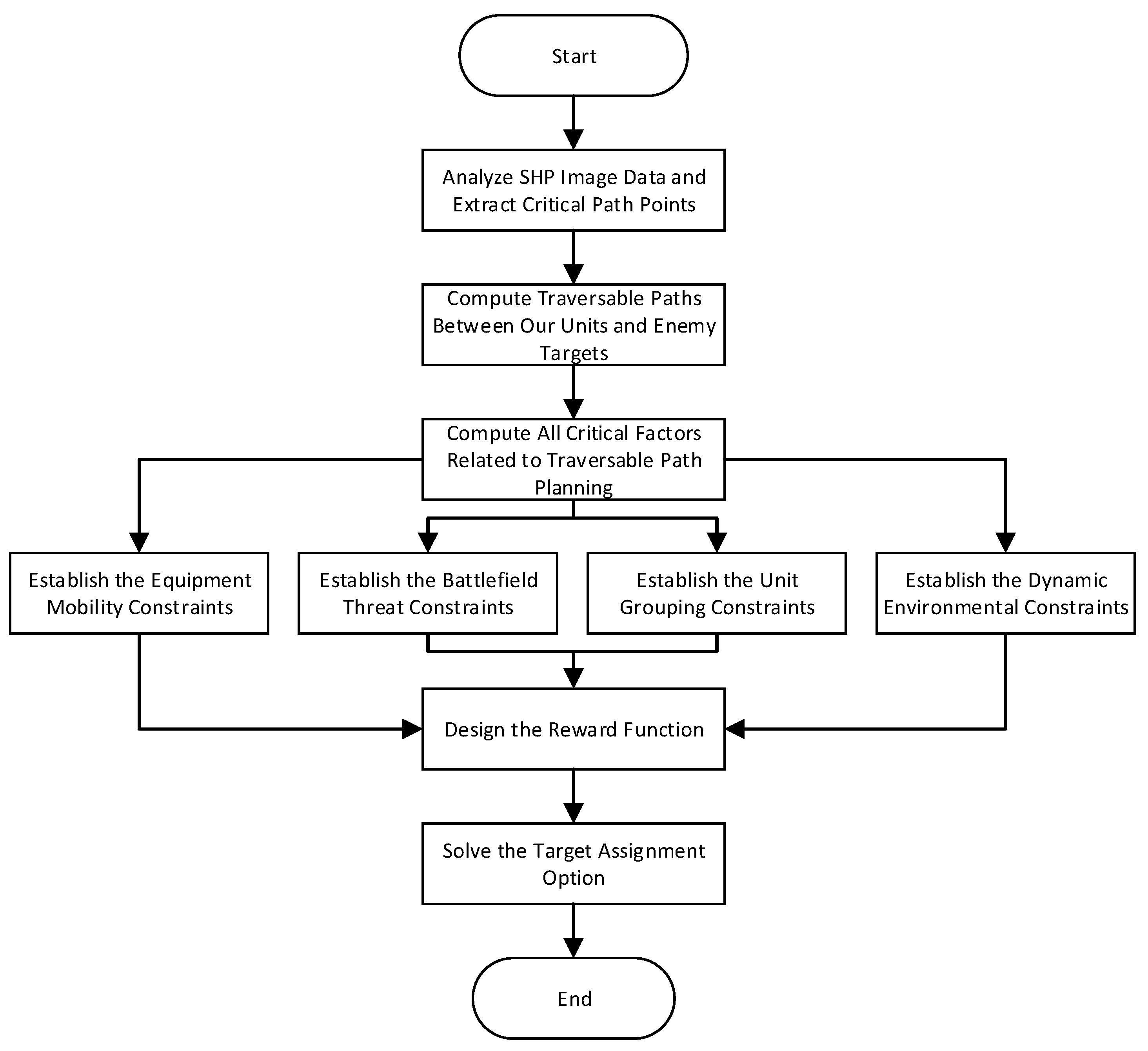
We focus on modeling and solving the target assignment problem in an urban environment. Specifically, the proposed approach proceeds through the following stages: First, to understand the operational area, we analyze a specific adversarial zone. This analysis extracts essential features of the urban road network and identifies critical path points. Second, leveraging real-time battlefield awareness, we gather positions, types, and attributes of our units and enemy targets along with the critical points. Using this comprehensive situational data, we then identify multiple traversable paths between our units and enemy targets. For each identified path, we compute critical performance factors: total distance, congestion level, threat level, and so on. Third, to optimize the assignment and movement, we construct constraint models and design a specialized reward function. These components work together to jointly optimize the grouping strategies and maneuvering strategies. Finally, based on this optimization, the method generates an effective target assignment plan. The overall workflow is summarized in Figure 1.

4.1. Image Acquisition and Analysis with Critical Path Point Extraction

This study uses Shapefile (SHP) data to build a geospatial database. SHP is an industry-standard format. It provides robust vector data management capabilities. SHP supports points, lines, and polygons. It also stores rich attribute data. This capability enables precise representation of critical urban elements. These elements include building footprints, road networks, and target-specific locations [40]. Furthermore, standardized SHP datasets are widely available. They are accessible through open source platforms like OpenStreetMap [41]. This accessibility facilitates the rapid construction of urban adversarial battlefield environment databases. It also significantly lowers data acquisition barriers.

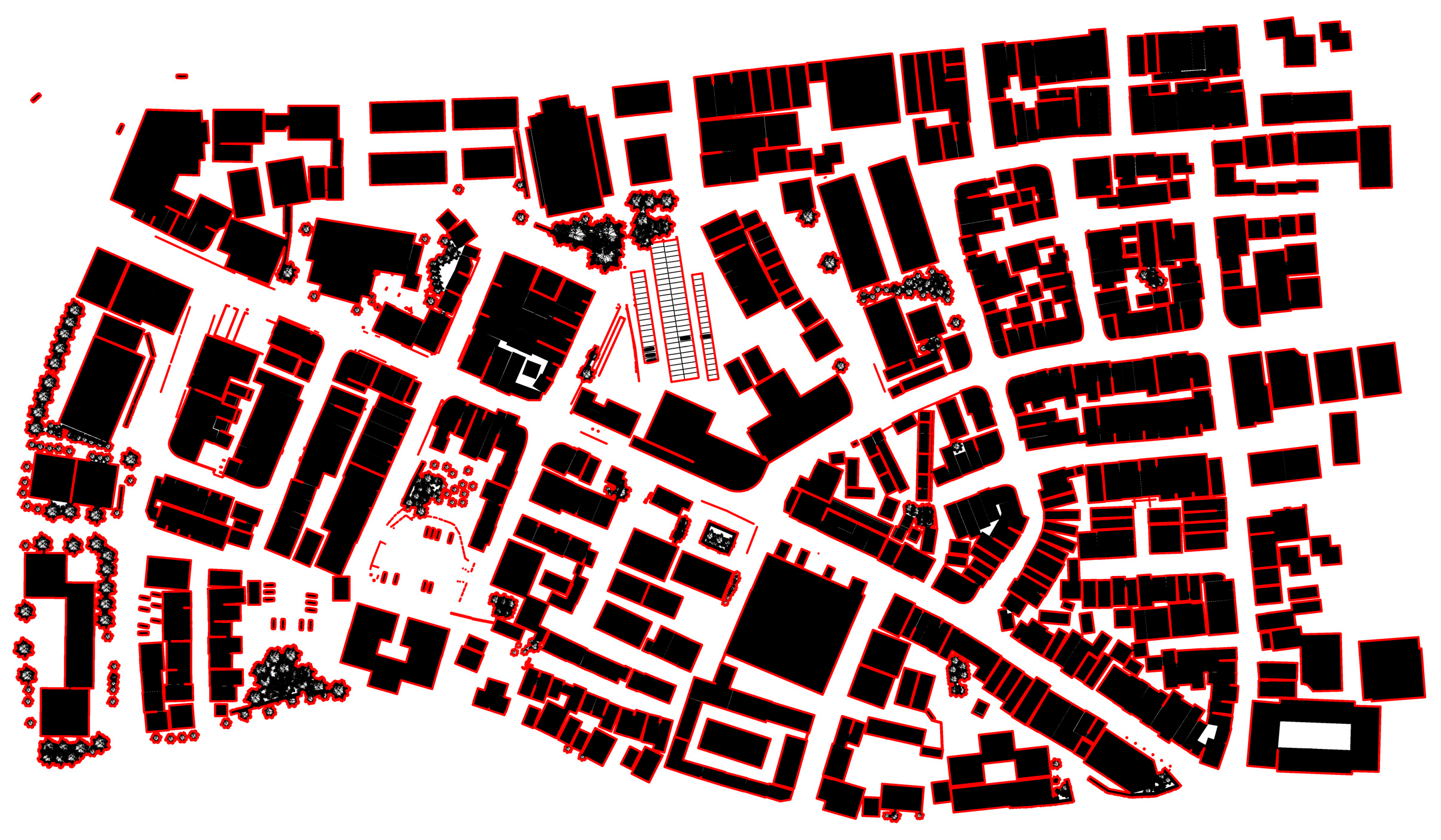
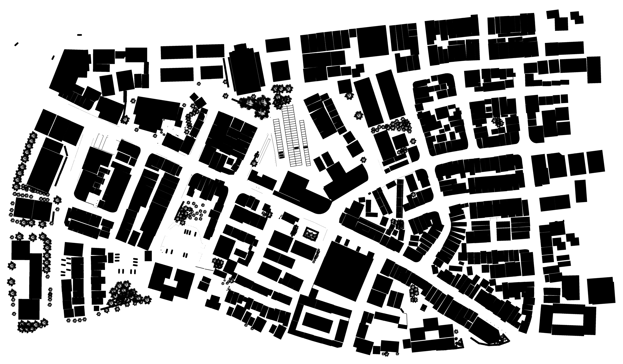
Core decision factors in target assignment depend fundamentally on horizontal spatial relationships. These factors include our units’ and enemy targets’ positions. They also include fire coverage ranges, line-of-sight areas, and maneuvering paths [42,43,44]. Consequently, this study employs a two-dimensional top-down perspective. This perspective serves as the primary analytical framework. It effectively avoids the visual distractions and computational complexity of three-dimensional space. This streamlines target assignment in an urban environment. The original SHP image data of the urban environment comes from UAV aerial photography. Therefore, the proposed method will also be adapted to real-world geospatial data. First, we render building polygons from the SHP data as a grayscale image where building interiors as black (0) and navigable areas as white (255). After that, we use adaptive Gaussian thresholding binarization to convert this data into a binary image:

$$T(x,y)={\displaystyle \frac{1}{k^2}}{\displaystyle \sum _{i=-h}^h{\displaystyle \sum _{j=-h}^{h}I(x+i,y+j)\cdot G(i,j)-C}}$$

(4)

where $T(x,y)$ denotes the local threshold, $I(x+i,y+j)$ denotes the original image’s grayscale value, $G(i,j)$ denotes the Gaussian kernel weight, $k$ denotes the neighborhood window size, and $C$ denotes the threshold offset. The converted image is shown in Figure 2.

After binarization, we extract polygonal contours using chain code and bounding box techniques. These contours capture urban road networks and building structures, as shown in Figure 3. We then apply geometric simplification with the Douglas–Peucker algorithm. The tolerance parameter $ϵ=1$ pixel reduces computational complexity while preserving critical spatial features. The algorithm iteratively eliminates non-essential vertices. For each baseline segment, it evaluates the maximum perpendicular distance $D$ from intermediate points to baseline segments:

$$D={\displaystyle \frac{\left|(y_2-y_1)x_0-(x_2-x_1)y_0+x_2{y}_1-y_2{x}_1\right|}{\sqrt{{(y_2-y_1)}^2+{(x_2-x_1)}^2}}}$$

(5)

Then, the vertices of the simplified polygon are extracted and saved as critical path points.

4.2. Connectivity Analysis and Traversable Path Computation

After extracting path points, we must determine their mutual connectivity. For any two points, we compute the differences in their horizontal and vertical coordinates $\left(\Delta x,\Delta y\right)$. We take the maximum of these values as the number of sampling points $n$ between them. A uniform set of intermediate points is then sampled along the connecting line segment. Each sampled coordinate is rounded to the nearest integer. We then check all sampled points: if any point corresponds to a black pixel in the binary image, the two points are disconnected. Black pixels indicate obstacles or non-traversable areas. Otherwise, the points are connected.

After determining connectivity among all points, we employ the A* algorithm. This algorithm generates traversable paths between our units and enemy units. As an efficient heuristic search method, A* guides its search using a cost function. The cost function $f\left(n\right)$ combines the actual and estimated costs:

$$f\left(n\right)=g\left(n\right)+h\left(n\right)$$

(6)

where $g\left(n\right)$ represents the actual cost from the start node to the current node $n$, and $h\left(n\right)$ is the estimated cost from node $n$ to the goal. This approach significantly reduces unnecessary node expansions, enabling the rapid generation of multiple traversable paths within complex urban road networks.

4.3. Constraint Model Design

We ensure the constraint model design aligns closely with urban combat characteristics and decision logic. To capture inherent environmental complexities, this study establishes four core constraint models: equipment mobility constraints, battlefield threat constraints, unit grouping constraints, and dynamic environmental constraints [45,46,47,48].

Table 2. Constraint models and related factors.

$\mathbf{Equipment}\mathbf{Mobility}\mathbf{Constraints}\mathit{t}\left(\mathit{j}\right)$	$\mathbf{Battlefield}\mathbf{Threat}\mathbf{Constraints}\mathit{M}(\mathit{j})$	$\mathbf{Unit}\mathbf{Grouping}\mathbf{Constraints}{\mathit{s}}_{\mathit{f}\mathit{o}\mathit{r}\mathit{c}\mathit{e}}$	$\mathbf{Dynamic}\mathbf{Environmental}\mathbf{Constraints}\mathit{D}\mathit{e}(\mathit{j})$
equipment type	equipment criticality $Im\left(i\right)$	equipment type	day-night cycle effect $DNI(t)$
equipment mobility speed $t\left(j\right)$	path traversability $x\left(i,j,k\right)$	unit firepower $Z\left(i\right)$	real-time path update $P_{des}(i,j,k)$
path traversability $x\left(i,j,k\right)$	line-of-sight range $P(i,j)$	enemy firepower $Z_j^{*}$	communication node dynamic $web(i,j,k)$
road congestion level $c\left(i,j,k\right)$	path threat level $W(i,j,k)$	firepower differential $Z\left(i\right)-Z_j^{*}$	electromagnetic interference effect $Ele(i,j,k)$
logistical support impact $b{z}_{gain}$	composite protection computation $Df\left(i\right)$	grouping effectiveness $gain\left(j\right)$

summarizes key factors considered in each model.

Before building the constraint model, we must compute key path metrics. These metrics derive from real-time battlefield awareness in urban adversarial scenarios. The awareness integrates multi-source situational data. We design these indicators based on publicly available equipment parameters and rules.

The offensive firepower value $Z\left(i\right)$ of our unit $i$ is closely related to its unit type, and specifically satisfies the following condition:

$$Z\left(i\right)=\left\{\begin{array}{ll}z{h}_{atk}& ifzh\left(i\right)=1,hq\left(i\right)=0,zj\left(i\right)=0,bz\left(i\right)=0\\ h{q}_{atk}& ifzh\left(i\right)=0,hq\left(i\right)=1,zj\left(i\right)=0,bz\left(i\right)=0\\ z{j}_{atk}& ifzh\left(i\right)=0,hq\left(i\right)=0,zj\left(i\right)=1,bz\left(i\right)=0\\ b{z}_{atk}& ifzh\left(i\right)=0,hq\left(i\right)=0,zj\left(i\right)=0,bz\left(i\right)=1\end{array}\right.$$

(7)

where $z{h}_{atk}\in {ℝ}^{+}$ denotes the offensive firepower of command units, $h{q}_{atk}\in {ℝ}^{+}$ denotes the offensive firepower of logistics units, $z{j}_{atk}\in {ℝ}^{+}$ denotes the offensive firepower of armored units, and $b{z}_{atk}\in {ℝ}^{+}$ denotes the offensive firepower of support units. $Z^{\ast }\left(j\right)\in {ℝ}^{+}$ denotes the offensive firepower of the enemy target $j$.

The defensive capability value $Df\left(i\right)$ of our unit $i$ is also closely related to its unit type and specifically satisfies the following condition:

$$Df\left(i\right)=\left\{\begin{array}{ll}z{h}_{def}& ifzh\left(i\right)=1,hq\left(i\right)=0,zj\left(i\right)=0,bz\left(i\right)=0\\ h{q}_{def}& ifzh\left(i\right)=0,hq\left(i\right)=1,zj\left(i\right)=0,bz\left(i\right)=0\\ z{j}_{def}& ifzh\left(i\right)=0,hq\left(i\right)=0,zj\left(i\right)=1,bz\left(i\right)=0\\ b{z}_{def}& ifzh\left(i\right)=0,hq\left(i\right)=0,zj\left(i\right)=0,bz\left(i\right)=1\end{array}\right.$$

(8)

where $z{h}_{def}\in {ℝ}^{+}$ denotes the defensive capability of command units, $h{q}_{def}\in {ℝ}^{+}$ denotes the defensive capability of logistics units, $z{j}_{def}\in {ℝ}^{+}$ denotes the defensive capability of armored units, and $b{z}_{def}\in {ℝ}^{+}$ denotes the defensive capability of support units.

The priority level value $Im\left(i\right)$ of our unit $i$ specifically satisfies the following condition:

$$Im\left(i\right)=\left\{\begin{array}{cc}z{h}_{im}^{day}& ifzh\left(i\right)=1,hq\left(i\right)=0,zj\left(i\right)=0,bz\left(i\right)=0,day=1\\ z{h}_{im}^{night}& ifzh\left(i\right)=1,hq\left(i\right)=0,zj\left(i\right)=0,bz\left(i\right)=0,day=0\\ h{q}_{im}& ifzh\left(i\right)=0,hq\left(i\right)=1,zj\left(i\right)=0,bz\left(i\right)=0\\ z{j}_{im}& ifzh\left(i\right)=0,hq\left(i\right)=0,zj\left(i\right)=1,bz\left(i\right)=0\\ b{z}_{im}& ifzh\left(i\right)=0,hq\left(i\right)=0,zj\left(i\right)=0,bz\left(i\right)=1\end{array}\right.$$

(9)

The binary variable $day\in \left\{0,1\right\}$ indicates day-night conditions. $z{h}_{im}^{day}\in {ℝ}^{+}$ denotes the priority levels of command units during the daytime and $z{h}_{im}^{night}\in {ℝ}^{+}$ at night, $h{q}_{im}\in {ℝ}^{+}$ denotes the priority levels of logistics units, $z{j}_{im}\in {ℝ}^{+}$ denotes the priority levels of armored units, and $b{z}_{im}\in {ℝ}^{+}$ denotes the priority levels of support units.

4.3.1. Equipment Mobility Constraints

The equipment mobility constraint model directly responds to the physical limitations imposed by urban topography on unit deployment. Path traversability determines feasible deployment areas for different equipment types. Road congestion couples with equipment mobility speed, which further impacts task response timeliness. Additionally, the logistics supply radius acts as a hard constraint during task execution.

Actually, our unit cannot engage multiple enemy targets simultaneously. It must select one path from the traversable paths to initiate an attack. For $\forall i\in \left\{0,1,\dots ,N\right\}$, $x\left(i,j,k\right)$ satisfies the following condition:

$${\displaystyle \sum _{k=0}^L{\displaystyle \sum _{j=0}^{K}x\left(i,j,k\right)}\le 1}$$

(10)

Mobility efficiency requires the following key considerations: unit grouping configurations, selected path characteristics, and support unit availability. For $\forall i\in \left\{0,1,\dots ,N\right\}$ and $\forall k\in \left\{0,1,\dots ,L\right\}$, the travel time $t\left(j\right)\in {ℝ}^{+}$ for an our group moving toward enemy target $j$ must satisfy the following condition:

$$t\left(j\right)=\max \left({\displaystyle \frac{x\left(i,j,k\right)\ast c\left(i,j,k\right)}{b{z}_{num}\left(j\right)\ast b{z}_{gain}}}\right)$$

(11)

$b{z}_{num}\left(j\right)\in \mathbb{N}$ denotes the number of support units attacking enemy target $j$. A greater number of support units leads to higher mobility efficiency. $b{z}_{gain}\in {ℝ}^{+}$ represents the mobility efficiency gain per support unit.

4.3.2. Battlefield Threat Constraints

The root cause of the battlefield threat constraint model stems from the spatial non-uniformity of threats in an urban environment. The perceived distance from enemies must be combined with path exposure levels to determine threat values. Furthermore, equipment importance and its integrated protection capabilities significantly determine survival likelihood. Therefore, we design this constraint based on historical experience rules and probability.

Consequently, battlefield threat assessment requires the following key considerations: unit grouping configuration, priority level, composite defense capability, path traversability, line-of-sight coverage along the path, and cumulative path risk. For $\forall i\in \left\{0,1,\dots ,N\right\}$ and $\forall k\in \left\{0,1,\dots ,L\right\}$, the battlefield threat $M\left(j\right)\in {ℝ}^{+}$ for our unit $i$ advancing towards enemy target $j$ must satisfy the following condition:

$$M(j)={\displaystyle \sum _{k=0}^L{\displaystyle \sum _{i=0}^N\left(Im(i)\ast x(i,j,k)\ast P(i,j)\ast D(i,j,k)\ast W(i,j,k)/Df(i)\right)}}$$

(12)

$P(i,j)$ indicates path viability for our unit $i$ to attack enemy target $j$. $D(i,j,k)$ is the maximum exposure distance for our unit $i$ attacking enemy target $j$ via path $k$. $W(i,j,k)$ is the combined danger level of the path.

4.3.3. Adversarial Grouping Constraints

The adversarial grouping constraint model arises from the dynamic balance requirement in firepower confrontation between our units and enemy targets. When enemy firepower exceeds a threshold, it must be suppressed by our own units. This firepower gap then triggers formation size adjustments. Ultimately, these adjustments result in exponential firepower growth that reflects grouping efficiency.

Based on the above factors, the combined firepower of our units in a group must be comprehensively considered with respect to the grouping configuration and offensive capabilities of the units. To constrain the combined firepower within a reasonable range, the following constraint is established:

$$z_{\min }\ast Z_j^{*}\le {\displaystyle \sum _{k=0}^L{\displaystyle \sum _{i=0}^N\left(x(i,j,k)\ast Z\left(i\right)\right)}}\le z_{\max }\ast Z_j^{*}$$

(13)

$z_{\min }\in {ℝ}^{+}$ denotes the minimum ratio of the combined firepower of our units to the firepower of enemy target $j$, and $z_{\max }\in {ℝ}^{+}$ represents the maximum allowable ratio between them.

In addition, the remaining firepower value $s_{force}\in {ℝ}^{+}$ of all our groups must satisfy the following condition:

$$\begin{array}{c}{s}_{force}={\displaystyle \sum _{k=0}^L{\displaystyle \sum _{j=0}^K{\displaystyle \sum _{i=0}^N\left(x(i,j,k)\ast Z\left(i\right)+h{q}_{gain}\ast h{q}_{num}(j)\ast x(i,j,k)\ast Z\left(i\right)\right.}}}\\ \left.+z{h}_{gain}\ast gain(j)\ast z{h}_{num}(j)\ast x(i,j,k)\ast Z\left(i\right)-Z_j^{*}\right)\end{array}$$

(14)

$h{q}_{num}\left(j\right)\in \mathbb{N}$ denotes the number of logistics units among all our units that are attacking enemy target $j$; $h{q}_{gain}\in {ℝ}^{+}$ represents the gain in offensive firepower contributed by each logistics unit. $z{h}_{num}\left(j\right)\in \mathbb{N}$ denotes the number of command units attacking enemy target $j$, and $z{h}_{gain}\in {ℝ}^{+}$ represents the gain in offensive firepower contributed by each command unit. The binary variable $gain\left(j\right)$ indicates whether our units attacking enemy target $j$ can maintain communication with the command unit.

4.3.4. Dynamic Environmental Constraints

In real-world adversarial operations, it is essential to account for dynamically changing external disturbances. To this end, a dynamic environmental constraint model is constructed, which specifically incorporates four key factors: day–night cycle effect, communication node dynamics, real-time path update, and electromagnetic interference. The following subsections present the mathematical formulations and physical interpretations of each sub-model.

The day–night cycle directly affects the mobility efficiency and tactical choices of our units. Following the binary classification principle for adversarial effectiveness, we define the day–night constraint as follows:

$$DNI(t)=\left\{\begin{array}{ll} 1,& t=\mathrm{day}\\ 0.8,& t=\mathrm{night}\end{array}\right.$$

(15)

Communication node dynamics refers to the destruction of the communication infrastructure during operation. This destruction causes communication node failures and subsequent disconnection of communication links. The probability of communication loss is positively correlated with path length. This correlation simulates the cumulative effect of disturbances throughout the engagement. The following constraint is satisfied:

$$web(i,j,k)={\displaystyle \frac{dis(i,j,k)}{100+L_{\max }}}$$

(16)

Real-time path update refers to the need to select a new route when the originally chosen path becomes impassable. This occurs due to destruction during operation. The following constraint must be satisfied:

$$P_{des}(i,j,k)=1-e^{-W(i,j,k)}$$

(17)

Electromagnetic interference refers to active electronic jamming by enemies against our units during combat. Examples include communication disruption, GPS spoofing, and radar suppression. We introduce a critical time threshold to divide the mobility process into two phases: a linear interference accumulation phase ($t\le t_{th}$) and an exponential degradation phase ($t>t_{th}$). Coefficients $k_1$ and $k_2{e}^{c(i,j,k)-t_{th}}$ dynamically characterize these phases. Coefficient $k_1$ represents short-term adaptive interference coupling effects. Coefficient $k_2{e}^{c(i,j,k)-t_{th}}$ represents long-term systemic failure coupling effects. The following condition is satisfied:

$$Ele(i,j,k)=\left\{\begin{array}{ll} k_1·c(i,j,k)& c(i,j,k)\le t_{th}\\ k_2·e^{c(i,j,k)-t_{th}}+k_1·t_{th}& c(i,j,k)>t_{th}\end{array}\right.$$

(18)

Considering all the above factors, the dynamic environmental impact $De\left(j\right)\in {ℝ}^{+}$ on our units moving toward enemy unit $j$ must satisfy the following constraint:

$$De(j)={\displaystyle \sum _{k=0}^L{\displaystyle \sum _{i=0}^N\frac{1}{DNI(t)}·((\frac{1}{1+web(dis(i,j,k))})+P_{des}(i,j,k)+Ele(i,j,k))}}$$

(19)

These four constraint models simultaneously serve as the decision-making optimization objectives in this paper.

4.4. MDP Model Description

Incorporating the constraint models designed in this paper, the components of the MDP are formulated as follows:

4.4.1. State Space

In the target assignment environment, the state space $S_{tot}$ is a two-dimensional matrix. It contains the states of all our units. The first dimension’s length depends on four elements: enemy unit ID, selected path ID, our unit ID in one-hot encoding, and our unit coordinates. The second dimension’s length equals the number of our units. Its expression is as follows:

$$S_{tot}={[s_1,s_2,\cdots ,s_n]}^T$$

(20)

4.4.2. Action Space

An action branch is a tuple of length 2. It contains the enemy unit ID selected by our unit and the corresponding path ID. The full action space comprises all possible combinations of enemy unit IDs and path IDs. Its design format is multi-discrete:

$$A=[a_1,a_2,\cdots ,a_n]$$

(21)

4.4.3. Reward Function

The reward function achieves four objectives. First, it improves unit mobility efficiency. Second, it shortens maneuvering time. Third, it enhances firepower utilization. Fourth, it reduces battlefield threats to units. It also mitigates adverse effects from dynamic environmental changes.

Based on the constraint models described above, the reward function is defined as follows:

$$Reward=R_t+R_M+R_S+R_{De}$$

(22)

$$R_t=-{\beta }_1\ast {\displaystyle \sum _{j=0}^{K}t}(j)$$

(23)

$$R_M=-{\beta }_2\ast {\displaystyle \sum _{j=0}^{K}M}\left(j\right)$$

(24)

$$R_S={\beta }_3\ast s_{force}$$

(25)

$$R_{De}=-{\beta }_4\ast {\displaystyle \sum _{j=0}^{K}De}\left(j\right)$$

(26)

where ${\beta }_1$, ${\beta }_2$, ${\beta }_3$, and ${\beta }_4$ denote the weights corresponding to the rewards of the four modules. Different weight configurations reflect preferences for different operational requirements.

5. Algorithm

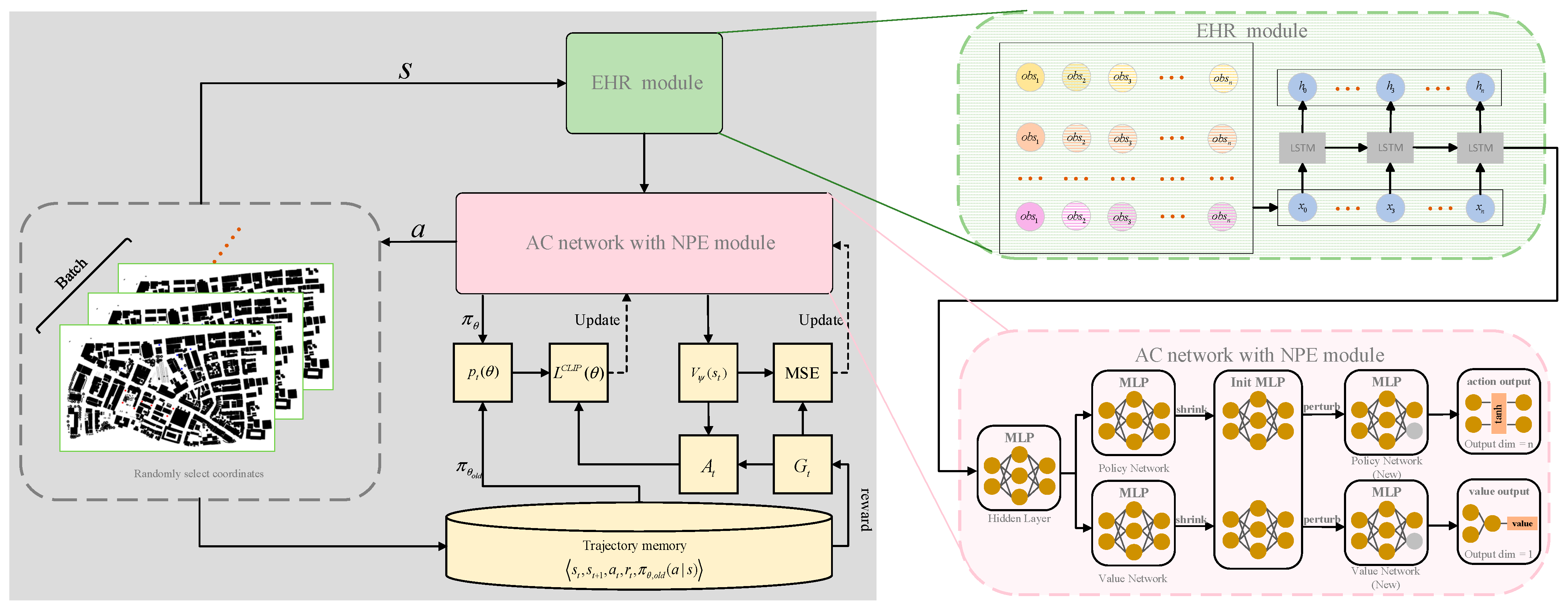
Urban adversarial target assignment must satisfy the complex constraints described earlier. Cross-dataset training introduces additional risks like parameter rigidity and policy oscillation. These significantly degrade traditional PPO algorithm performance. To solve these problems, we propose the GSPPO algorithm. Its architecture contains three core modules: an EHR module, an actor-critic joint network, and an NPE module. The EHR module constructs memory units across time steps. This encodes the characteristics of historical interaction trajectories. The actor-critic network uses EHR module outputs to generate target assignment policies and value estimations. The NPE mechanism applies gradient-based parameter shrinking and perturbation. This imposes continuous constraints on network weights. These modules collectively enhance algorithm generalization.

5.1. Design of EHR Module

Crucially, traversable path training datasets come from diverse initial state distributions. Yet, all data originate from the same adversarial environment. This environment consistency embeds spatial correlations. These correlations enable transferable implicit information patterns across datasets. This significantly enhances model generalization.

Urban adversarial target assignment exhibits strong temporal dependencies. Each unit–target matching decision directly impacts subsequent assignment outcomes. Using only single-time decision results in updates may trap policies in local optima. Therefore, incorporating historical environment interaction trajectories into every learning process enhances decision quality and efficiency. This sequential decision-making requires long-term temporal modeling capability. To address this, we integrate an EHR module into the PPO framework. The module constructs multi-timestep memory units that capture explicit temporal features from input sequences and extract implicit topological relationships in environmental data. This dual capability significantly enhances complex environment decision-making. The module input expands into temporal sequences by incorporating historical observations, which is formalized as follows:

$$y=[ob{s}_{t-m},\cdots ,ob{s}_{t-2},ob{s}_{t-1},ob{s}_t]$$

(27)

The module extracts valuable information from historical observation sequences. It feeds this information to subsequent layers, enhancing policy training. EHR integration enhances correlated information extraction from sequential data. This improves the policy network’s representation capability. The algorithm structure we designed is shown in Figure 4.

During training, EHR’s hidden state evolves with historical sequences. This captures time-varying hidden information. In contrast, traditional MLP-based policies lack recurrent memory. They optimize decisions using only current observations. Consequently, they underperform in stochastic tasks compared to recurrent policies. This demonstrates EHR’s superiority in sequential decision-making.

We summarize the EHR module in Algorithm 1.

Algorithm 1: EHR module of GSPPO algorithm

1: Initialize EHR states $h_0,c_0$ 2: for $t=1,2,\dots ,T_{\max }$ do 3:       for $i=1,2,\dots ,N_{env}$ do 4:             Store $〈o_t,h_t,c_t〉$ into replay buffer 5:             $a_t$,$v_t$,$〈h_{t+1},c_{t+1}〉$ = EHR $〈o_t,h_t,c_t〉$ 6: end for 7: Compute advantages with EHR′s final state 8: Train on sequences maintaining EHR state continuity

5.2. Design of NPE Module

Urban adversarial target assignment faces dual challenges during cross-dataset training: network rigidity and policy instability. First, model parameters gradually converge during training. Feature discrepancies across heterogeneous datasets meanwhile hinder network adaptation. Second, policy-value function divergence induces policy oscillation during frequent task switching. Therefore, the model must enhance its adaptability to new datasets while maintaining performance to represent old datasets.

To overcome these limitations, we propose an NPE module. NPE activates after each gradient update. This enables dynamic weight adjustment without periodic hyperparameter tuning. For the neurons in the network, NPE breaks the direct inheritance of prior-round parameters. Instead, it combines parameter shrinking with perturbed initialization. This alters gradient dynamics and update paths for new data.

The shrink operation reduces old-data reliance while amplifying new-data gradients. This balances gradient amplitudes across datasets. Simultaneously, perturbation disrupts old-data memory patterns to enhance new-data adaptability. These operations collectively enhance the plasticity of the network, thereby greatly improving its generalization ability across datasets.

For a parameter set $x$, the updated parameter set $x_{new}$ is computed according to the following formula:

$$x_{new}=\alpha x_{cur}+\beta x_{init}$$

(28)

where $x_{init}$ is sampled from the initial parameter distribution, $\alpha$ and $\beta$ are scaling coefficients that satisfy $\alpha =1-\beta$. This module directly regulates gradient balance during new data training. It balances gradient contributions between old and new data, which prevents generalization degradation caused by distribution shifts. The mathematical representation is as follows:

$$‖{\nabla }_{x_{new}}{L}_{new}(x_{new})‖\approx ‖{\nabla }_{x_{new}}{L}_{old}(x_{new})‖$$

(29)

where $L_{new}(x_{new})$ denotes the loss on new datasets under parameter set $x_{new}$, and $L_{old}(x_{new})$ denotes the loss on old datasets under $x_{new}$.

We summarize the NPE module in Algorithm 2.

Algorithm 2: NPE module of GSPPO algorithm

1: Initialize NPE module $\theta$ with ${\theta }_0$ 2: for epochs 1 to $N$ do 3:       Collect trajectories using ${\pi }_{\theta }$ 4:       Update $\theta$ via GSPPO gradient step 5:       for each parameter group $g\in T$ do  //$T=\left\{encoder,policy,value\right\}$ 6:       ${\theta }_{new}=\alpha {\theta }_{cur}+\beta {\theta }_{init}$ 7:       end for 8: end for

For large-scale exploration tasks, we use a multi-environment parallel framework. This coordinates shared network weight updates across multiple environments. The policy network runs synchronously in randomly initialized environments. It generates diverse trajectories. These form vast sample sets under the current policy. Stochastic gradient descent then optimizes this dataset iteratively. This reduces parameter update variance and accelerates convergence. It also improves convergence stability.

We summarize the proposed method in Algorithm 3.

Algorithm 3: GSPPO algorithm for Urban Adversarial Target Assignment

Input: observation sequence $y$ Output: target assignment plan

1: Initialize policy network, ${\pi }_{{\theta }_{old}}$, ${\pi }_{\theta }$ and value function $V_{\psi }(s_t)$ 2: for n = 1, 2, …, maximum training episode $N_{\max }$ do 3:     Initialize $N_{env}$ different workers randomly 4:     Calculate the learning rate lr and entropy bonus coefficient β  5:     for $t=1,2,\dots ,T_{\max }$ do 6:                 for $i=1,2,\dots ,N_{env}$ do 7:                          Run policy ${\pi }_{{\theta }_{old}}$, collect $\{o_i^t,r_i^t,a_i^t\}$ 8:                          Store $〈S_t,a_t,r_t,S_{t+1}〉$ into replay buffer 9:                 end for 10:                        Collect set of partial trajectories $D_t$ from different scenarios 11:                end for 12:                Divide $D_t$ into sequences of length $n_{len}$ 13:                Calculate advantage estimates $A_t$ 14:                for $k=1,2,\dots ,$ maximum GSPPO epochs $k_{\max }$ do 15:                        Calculate loss function $L(\theta )=L^{CLIP}(\theta )+\alpha L^{VF}(\theta )+\beta L^{ENT}(\theta )$ 16:                        Update weights via backpropagation 17:                 end for 18:                 Adjust network parameters using NPE 19: end for

6. Experiments and Analysis

This section presents the experiments conducted on the proposed work from four distinct perspectives. All experiments were conducted in Python 3.8 using PyTorch 1.8.0 and gym 0.26.2 within PyCharm 2023.1.2, running on hardware with an NVIDIA Quadro 5000 GPU (16 GB) and Intel i9-9960X CPU. Firstly, we compared the convergence curves of various RL algorithms on this task. Secondly, we verified the effectiveness of each designed module through ablation experiments. Subsequently, we evaluated the performance of our method against RL algorithms and GA. Finally, we analyzed reward weight impacts on policy generalization. These experiments collectively validate our approach comprehensively.

6.1. Comparative Experiment

In the aforementioned urban environment scenarios, traversable paths from diverse initial states form the training dataset. The proposed GSPPO method was applied for training. We defined three adversarial scenarios. Scenario 1: 7 vs. 4 forces with 20 traversable paths per unit–target pair. Scenario 2: 10 vs. 6 forces with 20 paths per pair. Scenario 3: 7 vs. 4 forces with 30 paths per pair. These configurations test scalability and path density impacts.

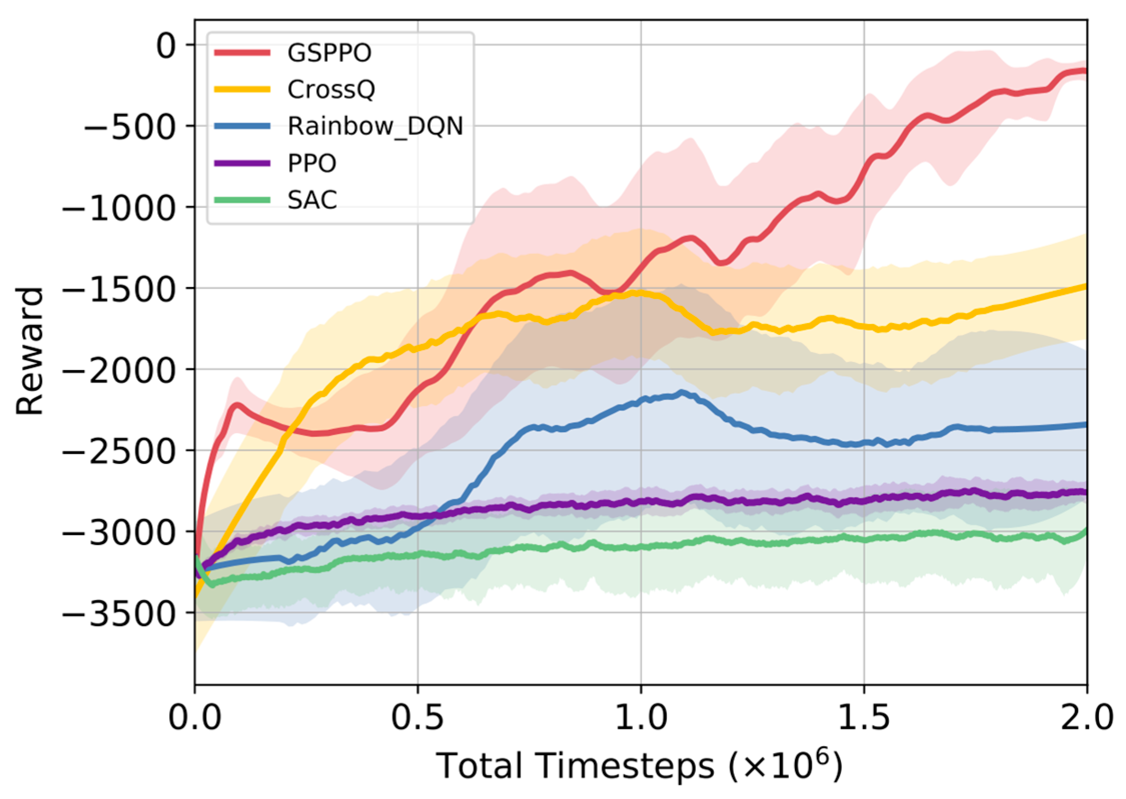
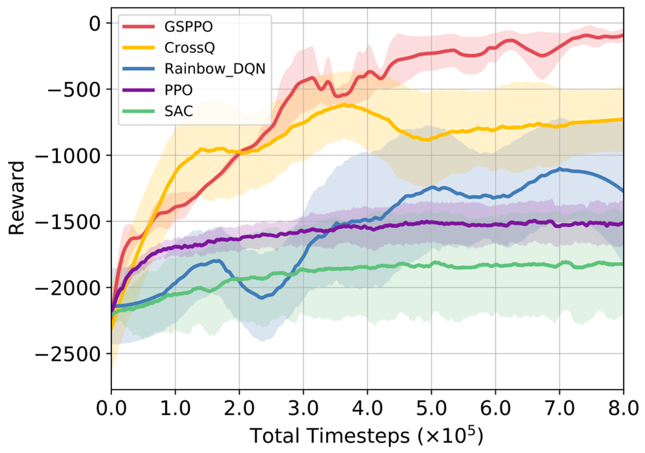
We also compared the proposed method with several RL algorithms in the experiments: the classic value-based algorithm Rainbow DQN [49], the actor-critic based algorithm SAC [50], and the relatively recent algorithm CrossQ [51]. The resulting learning curves after training are shown in Figure 5, Figure 6 and Figure 7.

The experiments use the theoretical optimum of each reward module as the benchmark. The reward equals the negative deviation from this benchmark. Thus, the theoretical maximum total reward is 0. As shown in Figure 5, GSPPO’s average reward increases steadily during training. It then plateaus near zero. This indicates policy network convergence.

Rainbow DQN, SAC, and CrossQ show low learning efficiency in urban adversarial scenarios. Their reward curves fail to approach the theoretical optimum. In contrast, GSPPO integrates two key innovations: an HER module and an NPE module. This integration improves data utilization and accelerates training convergence. It also mitigates performance disruptions from complex constraints and multi-dataset variations. Agents thus learn superior policies in challenging conditions.

Figure 6 shows that in scenario 2, GSPPO can still maintain high performance when facing scale expansion. Baseline algorithms exhibit significant degradation. This confirms GSPPO’s scalability for large-scale constrained target assignment.

Figure 7 displays the impact of increasing path density on the algorithm. From the results, it can be seen that though this expands the action space substantially, GSPPO maintains effective performance. This demonstrates generalization against combinatorial complexity.

6.2. Ablation Experiment

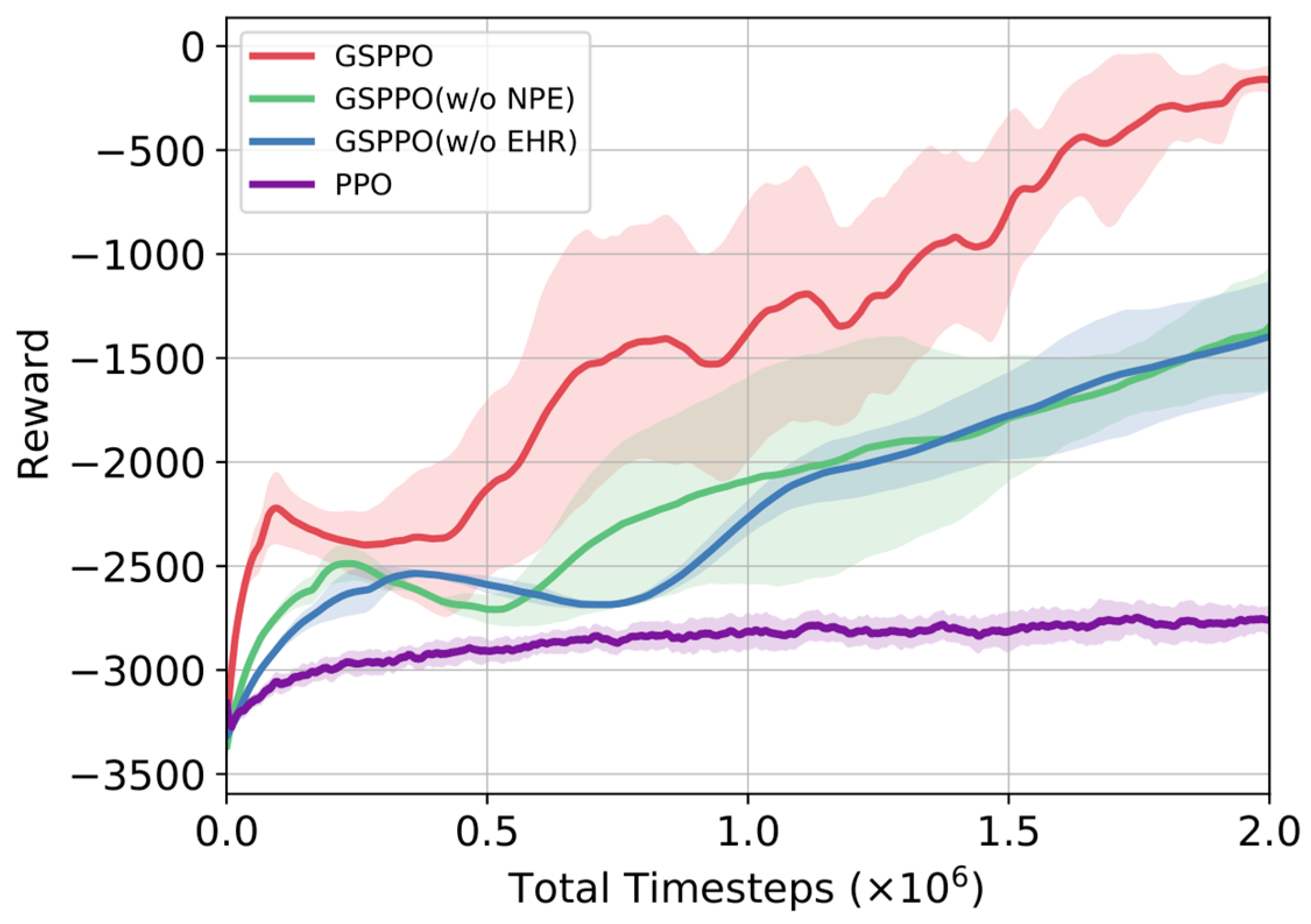
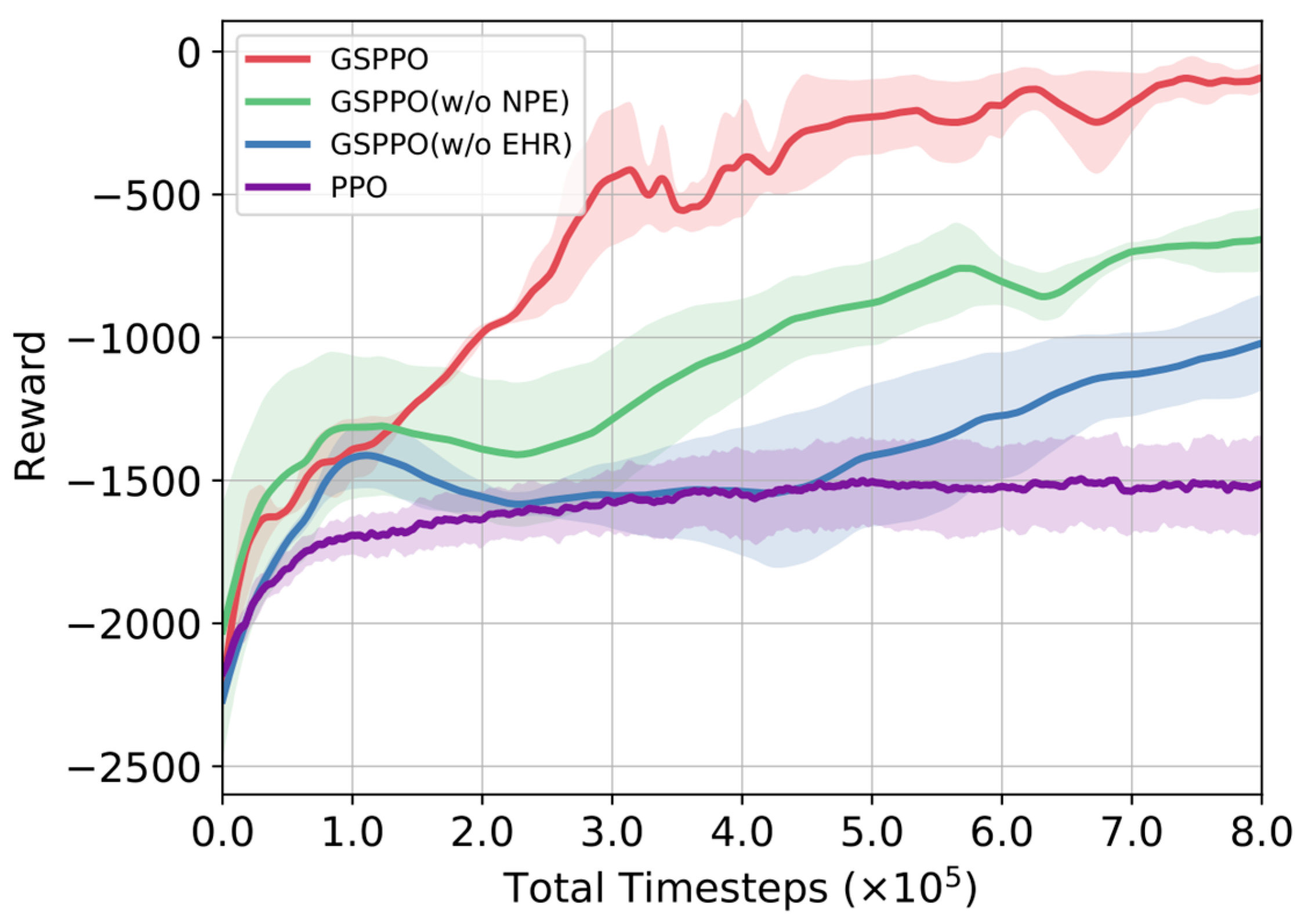
We introduced two improvements to the traditional PPO algorithm. To evaluate the impact of each component on overall performance, ablation experiments were conducted by removing one improvement at a time, and the algorithm’s performances were compared across the three aforementioned application scenarios, as shown in Figure 8, Figure 9 and Figure 10.

Ablation results demonstrate key insights. The full GSPPO (EHR + NPE) achieves optimal performance. Partial variants (w/o EHR or w/o NPE) still significantly outperform baseline PPO. Both variants yield higher rewards than PPO with comparable convergence speeds.

The EHR module captures temporal dependencies in urban target assignment. Its memory cells and gating mechanisms model long-term dynamics. This capability exceeds traditional PPO methods. EHR maintains decision consistency across time steps. It thereby improves cumulative rewards.

The NPE module mitigates network plasticity loss during multi-dataset training. It enhances the model’s representational capability and cross-task generalization. By injecting controlled noise into parameter updates, NPE improves generalization against input distribution shifts while preserving policy space continuity. EHR and NPE collaborate synergistically. Their integration enables strong generalization across diverse adversarial scenarios.

6.3. Policy Application Performance Comparison

We evaluated GSPPO in a 7 vs. 4 scenario with 20 traversable paths per unit–target pair. Performance metrics included path length, threat value, and total time. The results were compared with those of the RL algorithms CrossQ, Rainbow DQN, SAC, as well as an improved genetic algorithm, AGA [52].

Each method was evaluated using 100 Monte Carlo simulations, and the values of all metrics in the results were normalized, as shown in

Table 3. Generalization results of different algorithms.

Algorithm	Path Length	Threat Value	Total Time
GSPPO	3.8073	2.3587	3.3784
CrossQ	4.6881	3.6088	5.2842
Rainbow DQN	5.1942	3.9406	5.3791
SAC	6.2637	5.8793	6.0164
AGA	3.7096	2.8541	3.6333

. The experimental results show that the target assignment solution obtained using the GSPPO algorithm achieves an average path length of 3.8073, a threat value of 2.3587, and a total time of 3.3784. Compared with the RL algorithms CrossQ, Rainbow DQN, SAC, and the genetic algorithm AGA, GSPPO can find better target assignment solutions.

We also compared the solving time and CPU utilization of the proposed algorithm with those of the genetic algorithm, as shown in

Table 4. Comparison of solving time.

Per Pair Path Number	GSPPO(s)	AGA(s)
1	1	5
5	1	16
7	1	378
10	2	6254
20	6	>>22,734

and

Table 5. Comparison of CPU utilization.

Per Pair Path Number	GSPPO	AGA
1	21.2%	30.1%
5	25.6%	41.7%
7	25.3%	54.0%
10	28.2%	72.2%
20	28.8%	86.5%

. Each method was evaluated using 10 repeated simulations. The leftmost column indicates the number of traversable paths used in the planning process. Combining the results described above, it can be concluded that the trained model significantly reduces the planning time required and the CPU usage. Moreover, even when the initial situation changes, the proposed model can still be directly invoked to generate a better assignment solution without the need for replanning.

Furthermore, we found that the proposed method relies on complete UAV aerial imagery. This imagery enables accurate extraction of traversable paths and critical path points. These elements underpin the target assignment framework. However, real-world urban environments often present challenges. Incomplete geospatial data are common, such as missing road segments or occlusions from foliage and buildings. Noisy UAV imagery also occurs, for example, due to inconsistent lighting. These issues may reduce solution reliability. The method’s performance requires full aerial coverage. Incomplete images can lead to unsatisfactory path extraction, resulting in suboptimal target assignment schemes being generated.

6.4. Parameter Sensitivity Analysis

We analyzed reward weight impacts on four operational objectives: mobility efficiency, battlefield threat, remaining firepower, and dynamic environmental factors. Four weight configurations emphasize different aspects of the operational objectives. This reveals how reward shaping quantitatively influences target assignment outcomes.

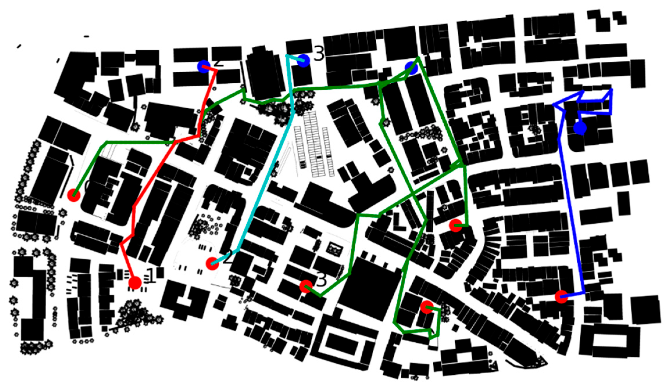
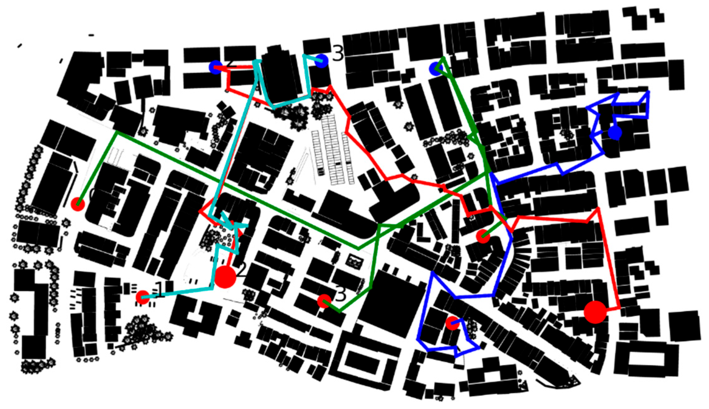
When ${\beta }_1=0.7,{\beta }_2=0.1,{\beta }_3=0.1,{\beta }_4=0.1$, the generated grouping and maneuver strategy is shown in Figure 11. Our units 0, 1, 4, and 5 form a single group and advance along the planned route to engage enemy target 2. Our unit 2 forms a separate group and advances along the planned route to engage enemy target 1. Our unit 3 forms another individual group and follows its planned route to attack enemy target 3. Our unit 6 also operates independently and advances toward enemy target 0 along its designated path.

The results indicate that when ${\beta }_1=0.7,{\beta }_2=0.1,{\beta }_3=0.1,{\beta }_4=0.1$, our units prioritize mobility efficiency during the offensive, with less consideration given to battlefield threat, remaining firepower, and dynamic environmental factors. This configuration emphasizes eliminating enemy units in the shortest possible time.

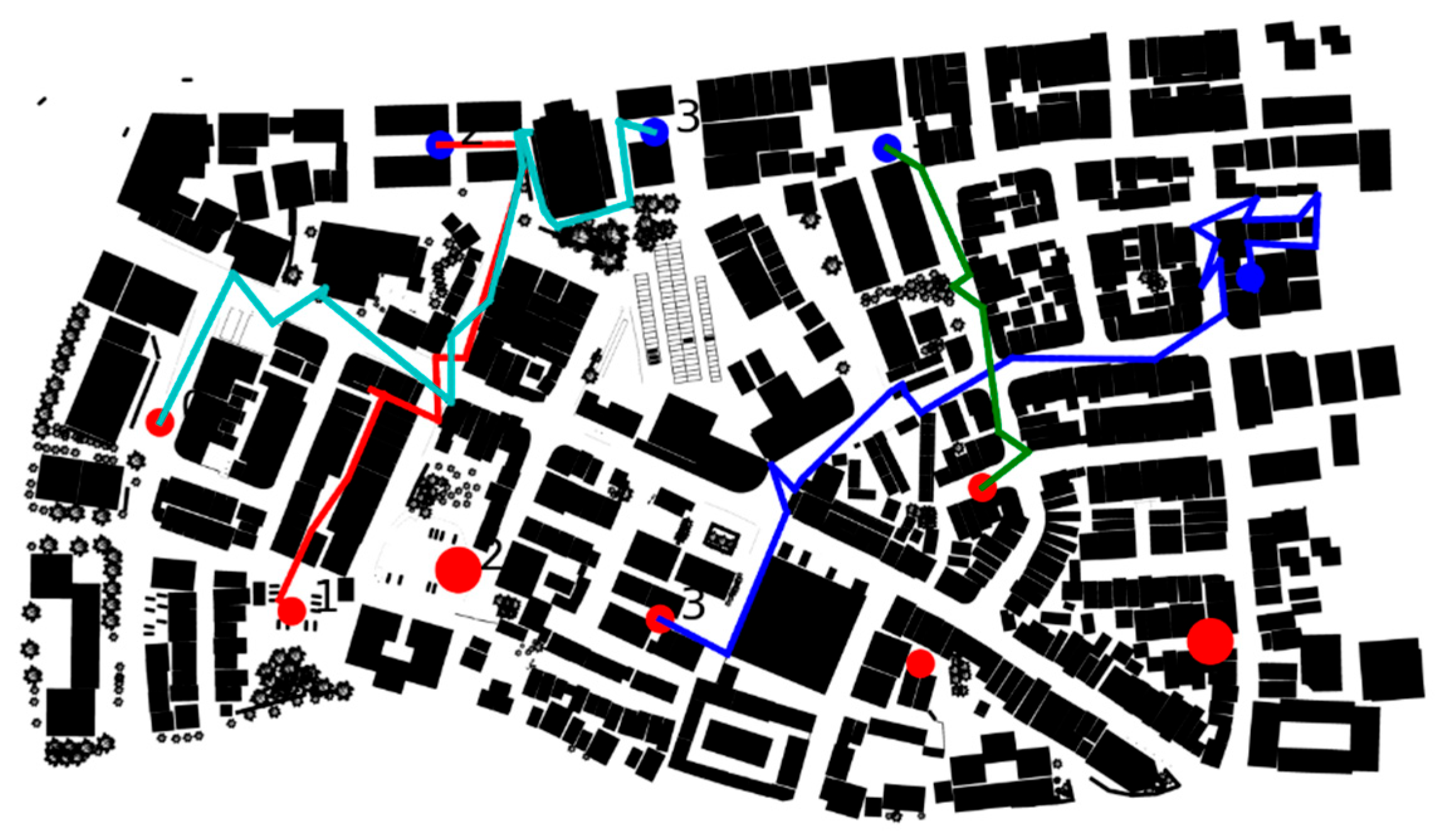
When ${\beta }_1=0.1,{\beta }_2=0.7,{\beta }_3=0.1,{\beta }_4=0.1$, the generated grouping and maneuver strategy is shown in Figure 12. Our units 0, 3, 4, and 5 form a single group and advance along the planned route to engage enemy target 1. Our unit 1 operates independently and advances along the planned route to attack enemy target 2. Our unit 2 forms another individual group and follows its designated path to engage enemy target 3. Our unit 6 also acts alone, advancing toward enemy target 0 along its planned route.

The results indicate that when ${\beta }_1=0.1,{\beta }_2=0.7,{\beta }_3=0.1,{\beta }_4=0.1$, our units prioritize reducing the potential threat encountered during maneuvering, thereby minimizing losses to our assets during the offensive.

When ${\beta }_1=0.1,{\beta }_2=0.1,{\beta }_3=0.7,{\beta }_4=0.1$, the generated grouping and maneuver strategy is shown in Figure 13. Our unit 0 operates independently and advances along the planned route to engage enemy target 3. Our unit 1 forms another individual group and follows its planned route to attack enemy target 2. Our unit 3 acts alone and advances toward enemy target 0. Our unit 5 also forms a separate group and moves along its designated path to engage enemy target 1. Meanwhile, units 2, 4, and 6 are not assigned any target and remain in a reserve state.

The results indicate that when ${\beta }_1=0.1,{\beta }_2=0.1,{\beta }_3=0.7,{\beta }_4=0.1$, our units prioritize maintaining a larger reserve force during the offensive, aiming to maximize the utilization of available firepower resources.

When ${\beta }_1=0.1,{\beta }_2=0.1,{\beta }_3=0.1,{\beta }_4=0.7$, the generated grouping and maneuver strategy is shown in Figure 14. Our units 0, 3, and 5 form a group and advance along the planned route to engage enemy target 1. Our unit 1 operates independently and advances along the planned route to attack enemy target 3. Our units 2 and 6 form another group and follow their respective paths to engage enemy target 2. Our unit 4 acts alone and advances toward enemy target 0 along its designated route.

The results indicate that when ${\beta }_1=0.1,{\beta }_2=0.1,{\beta }_3=0.1,{\beta }_4=0.7$, our units prioritize strategies that are less susceptible to disruption. This configuration aims to minimize the negative impact of potential dynamic disturbances in the operational environment.

The reward weight sensitivity analysis reveals distinct behavioral shifts in target assignment strategies based on parameter configurations. Prioritizing mobility efficiency ${\beta }_1$ minimizes engagement time but increases vulnerability to threats. Emphasizing threat reduction ${\beta }_2$ enhances survivability at the cost of operational speed. Maximizing reserve firepower ${\beta }_3$ conserves resources but may delay mission completion. Optimizing for environmental adaptability ${\beta }_4$ improves disturbance resistance while requiring balanced trade-offs in other objectives. These results demonstrate that strategic preferences can be systematically encoded through weight adjustments, enabling mission-specific policy customization. The framework’s flexibility supports diverse operational requirements—from time-critical strikes to high-risk reconnaissance—by modulating the relative importance of core constraints within the reward function.

7. Conclusions

This paper establishes an integrated target assignment framework for urban environments without road networks, which is initiated with traversable path generation from binarized SHP data, progressing to MDP modeling solved by our novel GSPPO algorithm. GSPPO intrinsically integrates the EHR module and the NPE module. EHR incorporates historical exploration trajectories into policy learning, significantly improving decision efficiency. NPE maintains neural plasticity through dynamic parameter recalibration, enhancing cross-scenario generalization. This synergy enables simulation-based real-time planning under complex constraints. Furthermore, a multi-environment parallel training approach is adopted to improve data efficiency and accelerate the learning process. The framework is applicable to military operations and shows potential in humanitarian tasks like disaster zone search/rescue, high-risk urban evacuation, and resource logistics under geospatial uncertainty.

Experimental validation against Rainbow DQN, SAC, CrossQ, and AGA demonstrated GSPPO’s superior solution efficiency. Against the benchmark algorithm, GSPPO achieves 94.16% higher convergence performance, 33.54% shorter assignment paths, 51.96% lower threat exposure, and 40.71% faster total time. The impact of different reward weight designs on the target assignment outcomes is also evaluated, demonstrating the effectiveness of each constraint model’s corresponding reward shaping in the overall reward function.

We found that the approach exhibits a certain limitation: reliance on complete UAV imagery. Moreover, the deployment in tactical contexts raises ethical concerns, including accountability for autonomous decisions and risks of civilian harm. Future work will focus on further developing robust preprocessing methods for real-world noisy data, implementing real-world validation with UGVs and LiDAR sensors, integrating RL methods capable of adapting to varying operational scales, as well as minimizing ethical impacts.

References

1. Li, X.J.; Zhang, D.D.; Yang, Y.; Zhang, H.X. Analysis on experienced lessons and core capabilities of urban operation. Prot. Eng. 2020, 42, 64–69. [Google Scholar]
2. Wei, N.; Liu, M.Y. Target allocation decision of incomplete information game based on Bayesian Nash equilibrium. J. Northwest. Polytech. Univ. 2022, 40, 755–763. [Google Scholar] [CrossRef]
3. Ou, Q.; He, X.Y.; Tao, J.Y. Overview of cooperative target assignment. J. Syst. Simul. 2019, 31, 2216–2227. [Google Scholar]
4. Li, K.P.; Liu, T.B.; Ram Kumar, P.N.; Han, X.F. A reinforcement learning-based hyper-heuristic for AGV task assignment and route planning in parts-to-picker warehouses. Transp. Res. Part E Logist. Transp. Rev. 2024, 185, 103518–103544. [Google Scholar] [CrossRef]
5. Ma, Y.; Wu, L.; Xu, X. Cooperative Targets Assignment Based on Multi-Agent Reinforcement Learning. Syst. Eng. Electron. 2023, 45, 2793–2801. [Google Scholar]
6. Moon, S.H. Weapon Effectiveness and the Shapes of Damage Functions. Def. Technol. 2021, 17, 617–632. [Google Scholar] [CrossRef]
7. Cheng, Y.Z.; Zhang, P.C.; Cao, B.Q. Weapon Target Assignment Problem Solving Based on Hungarian Algorithm. Appl. Mech. Mater. 2015, 3744, 2041–2044. [Google Scholar] [CrossRef]
8. Andersen, A.C.; Pavlikov, K.; Toffolo, T.A.M. Weapon-target assignment problem: Exact and approximate solution algorithms. Ann. Oper. Res. 2022, 312, 581–606. [Google Scholar] [CrossRef]
9. Guo, W.K.; Vanhoucke, M.; Coelho, J. A Prediction Model for Ranking Branch-and-Bound Procedures for the Resource-Constrained Project Scheduling Problem. Eur. J. Oper. Res. 2023, 306, 579–595. [Google Scholar] [CrossRef]
10. Ni, M.F.; Yu, Z.K.; Ma, F.; Wu, X.R. A Lagrange Relaxation Method for Solving Weapon-Target Assignment Problem. Math. Probl. Eng. 2011, 2011, 873292. [Google Scholar] [CrossRef]
11. Su, J.; Yao, Y.; He, Y. Studying on Weapons-Targets Assignment Based on Genetic Algorithm. In Proceedings of the 2nd International Symposium on Computer Science and Intelligent Control, Stockholm, Sweden, 21–23 September 2018; pp. 1–5. [Google Scholar]
12. Zhai, H.; Wang, W.; Li, Q.; Zhang, W. Weapon-Target Assignment Based on Improved PSO Algorithm. In Proceedings of the 2021 33rd Chinese Control and Decision Conference (CCDC), Kunming, China, 22–24 May 2021; pp. 6320–6325. [Google Scholar]
13. Cao, M.; Fang, W. Swarm Intelligence Algorithms for Weapon-Target Assignment in a Multilayer Defense Scenario: A Comparative Study. Symmetry 2020, 12, 824. [Google Scholar] [CrossRef]
14. Huang, J.; Li, X.; Yang, Z.; Kong, W.; Zhao, Y.; Zhou, D. A Novel Elitism Co-Evolutionary Algorithm for Antagonistic Weapon-Target Assignment. IEEE Access 2021, 9, 139668–139684. [Google Scholar] [CrossRef]
15. Bengio, Y.; Lodi, A.; Prouvost, A. Machine Learning for Combinatorial Optimization: A Methodological Tour d’horizon. Eur. J. Oper. Res. 2021, 290, 405–421. [Google Scholar] [CrossRef]
16. Mouton, H.; Le Roux, H.; Roodt, J. Applying reinforcement learning to the weapon assignment problem in air defence. Sci. Mil. S. Afr. J. Mil. Stud. 2011, 39, 99–116. [Google Scholar] [CrossRef]
17. Li, S.; Jia, Y.; Yang, F.; Qin, Q.; Gao, H.; Zhou, Y. Collaborative Decision-Making Method for Multi-UAV Based on Multiagent Reinforcement Learning. IEEE Access 2022, 10, 91385–91396. [Google Scholar] [CrossRef]
18. Chen, W.; Zhang, Z.; Tang, D.; Liu, C.; Gui, Y.; Nie, Q.; Zhao, Z. Probing an LSTM-PPO-Based Reinforcement Learning Algorithm to Solve Dynamic Job Shop Scheduling Problem. Comput. Ind. Eng. 2024, 197, 110633. [Google Scholar] [CrossRef]
19. Lian, S.; Zhang, F. A Transferability Metric Using Scene Similarity and Local Map Observation for DRL Navigation. IEEE/ASME Trans. Mechatron. 2024, 29, 4423–4433. [Google Scholar] [CrossRef]
20. Juliani, A.; Ash, J.T. A Study of Plasticity Loss in On-Policy Deep Reinforcement Learning. Adv. Neural Inf. Process. Syst. 2024, 37, 113884–113910. [Google Scholar]
21. Cha, Y.-H.; Kim, Y.-D. Fire Scheduling for Planned Artillery Attack Operations under Time-Dependent Destruction Probabilities. Omega 2010, 38, 383–392. [Google Scholar] [CrossRef]
22. Kline, A.G.; Ahner, D.K.; Lunday, B.J. Real-Time Heuristic Algorithms for the Static Weapon Target Assignment Problem. J. Heuristics 2019, 25, 377–397. [Google Scholar] [CrossRef]
23. Lu, Y.; Chen, D.Z. A New Exact Algorithm for the Weapon-Target Assignment Problem. Omega 2021, 98, 102138. [Google Scholar] [CrossRef]
24. Ahner, D.K.; Parson, C.R. Optimal Multi-Stage Allocation of Weapons to Targets Using Adaptive Dynamic Programming. Optim. Lett. 2015, 9, 1689–1701. [Google Scholar] [CrossRef]
25. Xin, B.; Wang, Y.; Chen, J. An Efficient Marginal-Return-Based Constructive Heuristic to Solve the Sensor–Weapon–Target Assignment Problem. IEEE Trans. Syst. Man Cybern. Syst. 2019, 49, 2536–2547. [Google Scholar] [CrossRef]
26. Xin, B.; Chen, J.; Zhang, J.; Dou, L.; Peng, Z. Efficient Decision Makings for Dynamic Weapon-Target Assignment by Virtual Permutation and Tabu Search Heuristics. IEEE Trans. Syst. Man Cybern. Part C (Appl. Rev.) 2010, 40, 649–662. [Google Scholar] [CrossRef]
27. Chang, T.; Kong, D.; Hao, N.; Xu, K.; Yang, G. Solving the Dynamic Weapon Target Assignment Problem by an Improved Artificial Bee Colony Algorithm with Heuristic Factor Initialization. Appl. Soft Comput. 2018, 70, 845–863. [Google Scholar] [CrossRef]
28. Zhang, K.; Zhou, D.; Yang, Z.; Li, X.; Zhao, Y.; Kong, W. A Dynamic Weapon Target Assignment Based on Receding Horizon Strategy by Heuristic Algorithm. J. Phys. Conf. Ser. 2020, 1651, 012062. [Google Scholar] [CrossRef]
29. Yan, Y.; Huang, J. Cooperative Output Regulation of Discrete-Time Linear Time-Delay Multi-Agent Systems under Switching Network. Neurocomputing 2017, 241, 108–114. [Google Scholar] [CrossRef]
30. Luo, W.; Lü, J.; Liu, K.; Chen, L. Learning-Based Policy Optimization for Adversarial Missile-Target Assignment. IEEE Trans. Syst. Man Cybern. Syst. 2022, 52, 4426–4437. [Google Scholar] [CrossRef]
31. Wang, T.; Fu, L.; Wei, Z.; Zhou, Y.; Gao, S. Unmanned Ground Weapon Target Assignment Based on Deep Q-Learning Network with an Improved Multi-Objective Artificial Bee Colony Algorithm. Eng. Appl. Artif. Intell. 2023, 117, 105612. [Google Scholar] [CrossRef]
32. Zou, S.; Shi, X.; Song, S. MOEA with Adaptive Operator Based on Reinforcement Learning for Weapon Target Assignment. Electron. Res. Arch. 2024, 32, 1498–1532. [Google Scholar] [CrossRef]
33. Ding, Y.; Kuang, M.; Shi, H.; Gao, J. Multi-UAV Cooperative Target Assignment Method Based on Reinforcement Learning. Drones 2024, 8, 562. [Google Scholar] [CrossRef]
34. Sutton, R.; Barto, A. Reinforcement Learning: An Introduction. IEEE Trans. Neural Netw. 1998, 9, 1054. [Google Scholar] [CrossRef]
35. Schulman, J.; Wolski, F.; Dhariwal, P.; Radford, A.; Klimov, O. Proximal Policy Optimization Algorithms. arXiv 2017, arXiv:1707.06347. [Google Scholar] [CrossRef]
36. Dohare, S.; Hernandez-Garcia, J.F.; Lan, Q.; Rahman, P.; Mahmood, A.R.; Sutton, R.S. Loss of Plasticity in Deep Continual Learning. Nature 2024, 632, 768–774. [Google Scholar] [CrossRef] [PubMed]
37. Nikishin, E.; Schwarzer, M.; D’Oro, P.; Bacon, P.-L.; Courville, A. The Primacy Bias in Deep Reinforcement Learning. In Proceedings of the 39th International Conference on Machine Learning, Baltimore, MD, USA, 17–23 July 2022; pp. 16828–16847. [Google Scholar]
38. Nikishin, E.; Oh, J.; Ostrovski, G.; Lyle, C.; Pascanu, R.; Dabney, W.; Barreto, A. Deep Reinforcement Learning with Plasticity Injection. In Proceedings of the 37th International Conference on Neural Information Processing Systems, New Orleans, LA, USA, 10–16 December 2023. [Google Scholar]
39. Ash, J.; Adams, R.P. On Warm-Starting Neural Network Training. In Proceedings of the Advances in Neural Information Processing Systems, Vancouver, BC, Canada, 6–12 December 2020; Curran Associates, Inc.: Red Hook, NY, USA, 2020; Volume 33, pp. 3884–3894. [Google Scholar]
40. Zhu, J.; Wang, X.; Wang, P.; Wu, Z.; Kim, M.J. Integration of BIM and GIS: Geometry from IFC to Shapefile Using Open-Source Technology. Autom. Constr. 2019, 102, 105–119. [Google Scholar] [CrossRef]
41. Santos, L.B.L.; Jorge, A.A.S.; Rossato, M.; Santos, J.D.; Candido, O.A.; Seron, W.; de Santana, C.N. (Geo)Graphs—Complex Networks as a Shapefile of Nodes and a Shapefile of Edges for Different Applications. Available online: https://arxiv.org/abs/1711.05879v1 (accessed on 20 June 2025).
42. Wang, D.; Xin, B.; Wang, Y.; Zhang, J.; Deng, F.; Wang, X. Constraint-Feature-Guided Evolutionary Algorithms for Multi-Objective Multi-Stage Weapon-Target Assignment Problems. J. Syst. Sci. Complex. 2025, 38, 972–999. [Google Scholar] [CrossRef]
43. Zeng, H.; Xiong, Y.; She, J.; Yu, A. Task Assignment Scheme Designed for Online Urban Sensing Based on Sparse Mobile Crowdsensing. IEEE Internet Things J. 2025, 12, 17791–17806. [Google Scholar] [CrossRef]
44. Kline, A.; Ahner, D.; Hill, R. The Weapon-Target Assignment Problem. Comput. Oper. Res. 2019, 105, 226–236. [Google Scholar] [CrossRef]
45. Xiang, X.; Wu, K.; Ren, T.; Wang, L.; Xie, C. Analysis of the Construction of the Kill Chain in Man-Unmanned Collaborative Command for Small-Unit Urban Operations. In Proceedings of the 13th China Command and Control Conference, Beijing, China, 15–17 May 2025; pp. 137–142. [Google Scholar]
46. Zhao, Q.; Li, L.; Chen, X.; Hou, L.; Lei, Z. Research on the development strategy of intelligent weapon equipment for urban warfare based on SWOT and FAHP. Command Control Simul. 2025, 47, 93–100. [Google Scholar]
47. Zheng, W.; Li, Q.; Liu, W.; Fei, A.; Wang, F. Data-knowledge-driven metaverse modeling framework for urban warfare. J. Command Control 2023, 9, 23–32. [Google Scholar]
48. Li, H.; Yang, H.; Sheng, Z.; Liu, C.; Chen, Y. Multi-UAV collaborative distributed dynamic task allocation based on MAPPO. Control Decis. 2025, 40, 1429–1437. [Google Scholar]
49. Hessel, M.; Modayil, J.; Van Hasselt, H.; Schaul, T.; Ostrovski, G.; Dabney, W.; Horgan, D.; Piot, B.; Azar, M.; Silver, D. Rainbow: Combining Improvements in Deep Reinforcement Learning. In Proceedings of the Thirty-Second AAAI Conference on Artificial Intelligence and Thirtieth Innovative Applications of Artificial Intelligence Conference and Eighth AAAI Symposium on Educational Advances in Artificial Intelligence, New Orleans, LA, USA, 2–7 February 2018; Volume 32. [Google Scholar] [CrossRef]
50. Haarnoja, T.; Zhou, A.; Abbeel, P.; Levine, S. Soft Actor-Critic: Off-Policy Maximum Entropy Deep Reinforcement Learning with a Stochastic Actor. In Proceedings of the 35th International Conference on Machine Learning, Stockholm, Sweden, 10–15 July 2018; pp. 1861–1870. [Google Scholar]
51. Bhatt, A.; Palenicek, D.; Belousov, B.; Argus, M.; Amiranashvili, A.; Brox, T.; Peters, J. CrossQ: Batch Normalization in Deep Reinforcement Learning for Greater Sample Efficiency and Simplicity. In Proceedings of the Twelfth International Conference on Learning Representations, Vienna, Austria, 7–11 May 2024. [Google Scholar]
52. Ye, F.; Chen, J.; Tian, Y.; Jiang, T. Cooperative Task Assignment of a Heterogeneous Multi-UAV System Using an Adaptive Genetic Algorithm. Electronics 2020, 9, 687. [Google Scholar] [CrossRef]
Figure 1. Schematic diagram of the target assignment for an urban adversarial scenario.
Applsci 15 09630 g001
Figure 2. Binarized SHP image.
Applsci 15 09630 g002
Figure 3. Polygon contour extraction.
Applsci 15 09630 g003
Figure 4. The GSPPO algorithm structure.
Applsci 15 09630 g004
Figure 5. Performance curves for scenario 1 (5 random seeds).
Applsci 15 09630 g005
Figure 6. Performance curves for scenario 2 (5 random seeds).
Applsci 15 09630 g006
Figure 7. Performance curves for scenario 3 (5 random seeds).
Applsci 15 09630 g007
Figure 8. Performance curves for scenario 1 (5 random seeds).
Applsci 15 09630 g008
Figure 9. Performance curves for scenario 2 (5 random seeds).
Applsci 15 09630 g009
Figure 10. Performance curves for scenario 3 (5 random seeds).
Applsci 15 09630 g010
Figure 11. Option when β 1 = 0.7 , β 2 = 0.1 , β 3 = 0.1 , β 4 = 0.1 .
Applsci 15 09630 g011
Figure 12. Option when β 1 = 0.1 , β 2 = 0.7 , β 3 = 0.1 , β 4 = 0.1 .
Applsci 15 09630 g012
Figure 13. Option when β 1 = 0.1 , β 2 = 0.1 , β 3 = 0.7 , β 4 = 0.1 .
Applsci 15 09630 g013
Figure 14. Option when β 1 = 0.1 , β 2 = 0.1 , β 3 = 0.1 , β 4 = 0.7 .
Applsci 15 09630 g014