Article

Predicting Constitutive Behaviour of Idealized Granular Soils Using Recurrent Neural Networks

1
Department of Architecture and Civil Engineering, City University of Hong Kong, Hong Kong
2
Shenzhen Research Institute of City University of Hong Kong, Shenzhen 518000, China
*
Author to whom correspondence should be addressed.
Appl. Sci. 2025, 15(17), 9495; https://doi.org/10.3390/app15179495
Submission received: 23 July 2025 / Revised: 26 August 2025 / Accepted: 27 August 2025 / Published: 29 August 2025

Abstract

The constitutive modelling of granular soils has been a long-standing research subject in geotechnical engineering, and machine learning (ML) has recently emerged as a promising tool for achieving this goal. This paper proposes two recurrent neural networks, namely, the Gated Recurrent Unit Neural Network (GRU-NN) and the Long Short-Term Memory Neural Network (LSTM-NN), which utilize input parameters such as the initial void ratio, initial fabric anisotropy, uniformity coefficient, mean particle size, and confining pressure to establish the high-dimensional relationships of granular soils from micro to macro levels subjected to triaxial shearing. The research methodology consists of several steps. Firstly, 200 numerical triaxial tests on idealized granular soils comprising polydisperse spherical particles are performed using the discrete element method (DEM) simulation to generate datasets and to train and test the proposed neural networks. Secondly, LSTM-NN and GRU-NN are constructed and trained, and their prediction performance is evaluated by the mean absolute percentage error (MAPE) and R-square against the DEM-based datasets. The extremely low error values obtained by both LSTM-NN and GRU-NN indicate their outstanding capability in predicting the constitutive behaviour of idealized granular soils. Finally, the trained ML-based models are applied to predict the constitutive behaviour of a miniature glass bead sample subjected to triaxial shearing with in situ micro-CT, as well as to two extrapolated test sets with different initial parameters. The results show that both methods perform well in capturing the mechanical responses of the idealized granular soils.

1. Introduction

Granular materials play a critical role in many geotechnical engineering problems such as foundation failure, ground settlement, and slope stability [1,2,3,4,5]. Understanding the complex relationships between macro and micro mechanical responses of these materials under external loading is crucial [6]. Conventional plasticity-based methods for studying the constitutive behaviour of granular soils are becoming increasingly complex and require the calibration of numerous parameters, which often makes them impractical for use in engineering applications [7,8,9,10]. Physical experiments are also time-consuming and suffer from potential operational issues and equipment precision challenges [11]. Despite various attempts to develop constitutive models for granular soils, the development of a unified theoretical and experimental model remains a challenge [7].
Machine learning (ML) is an approach that relies on neural network algorithms to learn from datasets that are already generated by the physical system or its numerical model. ML, in contrast to traditional methods, is not predominantly reliant on theoretical assumptions or experimental designs. It primarily operates on a data-driven basis, utilizing mathematical techniques. This attribute allows ML to effectively map high-dimensional mechanical properties of granular soils, transcending the constraints of theoretical formulations [12], making it a powerful tool for a wide range of applications in the powder industry, geotechnical engineering, agriculture engineering, etc. [13,14,15]. In particular, the use of artificial neural network (ANN) models has proven effective in capturing nonlinear mechanical relationships of granular materials, such as the small-strain shear modulus affected by particle sizes and liquefaction resistance using a coupled approach that integrates the Lattice Boltzmann Method (LBM) and discrete element method (DEM) [16,17]. Extending this trend to earth-retaining systems, eXplainable Artificial Intelligence (XAI) has been used to classify failure mechanisms and estimate critical acceleration for flexible retaining walls using FEM-generated datasets, achieving state-of-the-art accuracy and millisecond-level inference while providing Shapley explanation (SHAP)-based interpretability [18]. Meanwhile, recent studies have demonstrated the potential of ML in predicting slope stability during earthquakes, as well as the dynamics of pore water pressure under varying rainfall conditions. For example, Gordan et al. [19] successfully combined an ANN with particle swarm optimization to predict the factor of safety of homogeneous slopes during earthquakes. Mustafa et al. [20] compared the performance of four ANN algorithms using the multilayer perception method to study the dynamics of pore water pressure under rainfall variations.
ANNs are known for their flexibility and computational efficiency in capturing intuitive relationships in granular soils. However, their simpler structure compared to other ML models makes them prone to challenges in handling sequential data and susceptible to overfitting [21]. Backpropagation Neural Networks (BPNNs) optimize weights and biases through error backpropagation from the output layer, aligning outputs with actual values [22]. However, traditional ML methods, including BPNNs, struggle with time-related nonlinear problems, lacking computational efficiency and precision.
Recurrent Neural Networks (RNNs) are a type of ML approach that excels in analyzing data that change over time, making them useful for a wide range of tasks. However, RNNs have limitations, such as the ‘gradient vanishing’ and ‘gradient explosion’ problems, which can lead to underfitting (where the model does not learn enough) or overfitting (where the model learns too much from the training data and does not perform well on new data). To improve upon RNNs, the Long Short-Term Memory Neural Network (LSTM-NN) was proposed by Hochreater and Schmidbuber [23] and later refined by Kawakami [24]. This version of an RNN was specifically designed to address the learning difficulties found in traditional RNNs, and it has achieved significant success in various applications. More recently, another innovative network called the Gated Recurrent Unit Neural Network (GRU-NN) has been developed. This network is particularly promising in language processing tasks. However, its potential in predicting how granular soils behave under different loading conditions is still being explored and is not yet fully established. Moreover, a detailed comparison is presented in Table 1, offering a structured overview of the key characteristics associated with several ML models, including ANN, BPNN, RNN, LSTM-NN, and GRU-NN.
In addition to the challenges faced by ML-based models, acquiring a sufficient amount of data to populate the dataset is also a significant obstacle. Previous research has shown that using the DEM simulations can enable the continuous observation of the microscopic responses of granular soils subjected to external loads [25]. The DEM serves as a bridge between macro and micro scales, facilitating the study of the microscopic mechanisms that underlie macroscopic mechanical properties [8,26].
This paper describes the use of two machine learning-based methods, namely, LSTM-NN and GRU-NN, along with a series of DEM simulations of triaxial tests, to capture the relationship between the deviatoric stress, mean stress, volumetric strain, fabric anisotropy evolution, and axial strain of idealized granular soils. For an enhanced analysis, we normalized the input data, in terms of the mean particle size, uniformity coefficient, initial fabric, initial void ratio, confining pressure, and axial strain in Python 3.9 to more accurately correlate it with key output variables. A comparative study on the quantitative predictions of the constitutive behaviour of granular soils between the proposed GRU-NN and LSTM-NN is presented, highlighting the differences in model performance and providing new insights for future research.

2. Methodology

2.1. DEM Simulations for Data Generation

Particle size distribution (PSD), which describes the size and composition proportion of particles within a soil sample, is an important parameter for characterizing the constitutive behaviour of granular soils at the microscale. In this study, we aim to generate idealized granular soils comprising polydisperse spherical particles to simplify the DEM simulations and enhance the computational efficiency. The PSD is determined by two grading characteristics: mean particle diameter (d50) and uniformity coefficient (Cu). Specifically, d50 represents the particle diameter at 50% in the cumulative distribution of PSD, and Cu is defined as the ratio of particle diameter d60 to particle diameter d10 (corresponding to 60% and 10% in the cumulative distribution of PSD, respectively) quoting from the principle of advanced soil mechanics [27]. Twenty granular samples with random combinations of the above two parameters were generated in a unified manner. We employed the fractal particle size distribution formula to tailor the number of particles in each granular sample accurately. This formula is given as F d = d 3 β d min 3 β / d max 3 β d min 3 β , where β represents the fractal dimension, influencing the ratio of different particle sizes. In our simulations, β is set to −1. The parameters dmax and dmin denote the maximum and minimum particle diameters in each sample, respectively. This approach, as elaborated in Ma et al. [6], ensures a reasonable and comparable number of particles across the samples. Typically, our samples contain approximately 3000 to 11,000 particles, with the variation accounting for differences in initial void ratios for medium dense and dense samples.
Figure 1 is designed to visually depict the process of generating particle size distributions characterized by various combinations of d50 and Cu for granular samples used in our simulations. In this figure, we employ a color-coding scheme in which each colour corresponds to a specific particle radius, displaying the realistic particle number under four typical conditions. This visual representation aims to clearly demonstrate how the particle size distribution is constructed, with decreasing sequence in particle number, for each granular sample. A total of 200 DEM simulations were conducted using samples with different PSDs, initial void ratios, and confining pressures. The ranges of the initial sample parameters used in this study are listed in Table 2. It should be noted that the initial fabric anisotropy was also calculated and used as an input parameter, and the focus of this paper is placed on the comparative study of LSTM-NN and GRU-NN in predicting the constitutive behaviour of idealized granular soils, so the effects of irregular particle shape are not considered in this study.
All simulations were performed using the commercial DEM software PFC3D 6.0 [28]. The simulation process of the triaxial test is described as follows. First, the idealized granular soil sample with a specified PSD was generated within a 16 mm (height) × 8 mm (diameter) cylindrical container which comprises two frictionless, rigid end platens and a lateral wall in favour of transmitting the vertical pressures through the radial confinement. Then, a constant confining pressure was applied to the cylindrical rigid wall, ranging from 100 kPa to 500 kPa, respectively, which was continuously adjusted by the servo-control system to maintain a desired stress level throughout the shearing process. Finally, two end platens were set to move relative to each other at a constant strain rate of 0.2% per minute while ensuring the loading rate was within the quasi-static range, until the axial strain of 15% was reached. The quasi-static loading condition is ensured by the dimensionless inertial number formula I =   ԑ a ˙ m / p , where ԑ a ˙ is the axial strain rate, m stands for the mass of the particle and p is the mean stress. Previous studies indicate that the inertial number should be less than 10−3 to maintain the quasi-static condition in DEM simulations [29,30]. Our calculations confirm that a loading rate of 0.2%/min satisfies this requirement. It is crucial that the quasi-static loading rate in numerical simulations is aligned with that of the physical experiment to ensure the DEM simulation accuracy. The 0.2%/min rate was chosen based on our prior research to mimic the loading rate used in the physical triaxial tests [22].
The DEM model parameters used are listed in Table 3. The Hertz–Mindlin contact model is a common choice to model the mechanical interactions of sand particles [31,32]. The inter-particle friction coefficient was set to 0.3, which is within the range of experimentally measured values of quartz sands [33,34]. To expedite quasi-static equilibrium and dissipate internal system energy, a local damping coefficient of 0.7 was used [35]. It should be noted that we adopt quartz-consistent values, including the shear modulus of 28 GPa and Poisson’s ratio of 0.25, as well as the particle density of 2650 kg/m3 following Wu et al. [26], who conducted a one-to-one model calibration against a micro-CT triaxial test and reported excellent agreement between the DEM model and the physical experiment [36].

2.2. Datasets Preparation and Pre-Processing

Figure 2 summarizes the workflow for the ML-based modelling process. Each particle size distribution (PSD) was assigned a unique identifier from 1 to 20. The symbols ‘D’ and ‘M’ were used to denote the dense samples and the medium dense samples, respectively, with the latter representing the relatively less dense samples in our numerical simulations. We have developed a comprehensive database to systematically investigate the effects of four initial soil packing state variables including initial mean particle size, initial uniformity coefficient, initial void ratio and initial fabric anisotropy, as well as two mechanical state parameters (confining pressure and axial strain) on the constitutive behaviour of granular soils, using 200 DEM-based simulations. For each simulation, 301 data points were recorded for the key mechanical responses, including deviatoric stress, mean stress, volumetric strain, and fabric anisotropy, all as functions of axial strain. In total, the database comprises 10 input and output variables and encompasses 240,800 normalized data pairs, thereby providing a robust foundation for data-driven constitutive modeling of idealized granular materials. Note that all of the data sequences start from the axial strain of 0% to the end of 15% and will be padded with a fixed length of 301. All variables in the raw dataset were normalized using min–max scaling in Python to scale each feature to a range of (0, 1). It should be noted that the amount of training data required for ML modelling remains a controversial issue without a definitive answer at present.
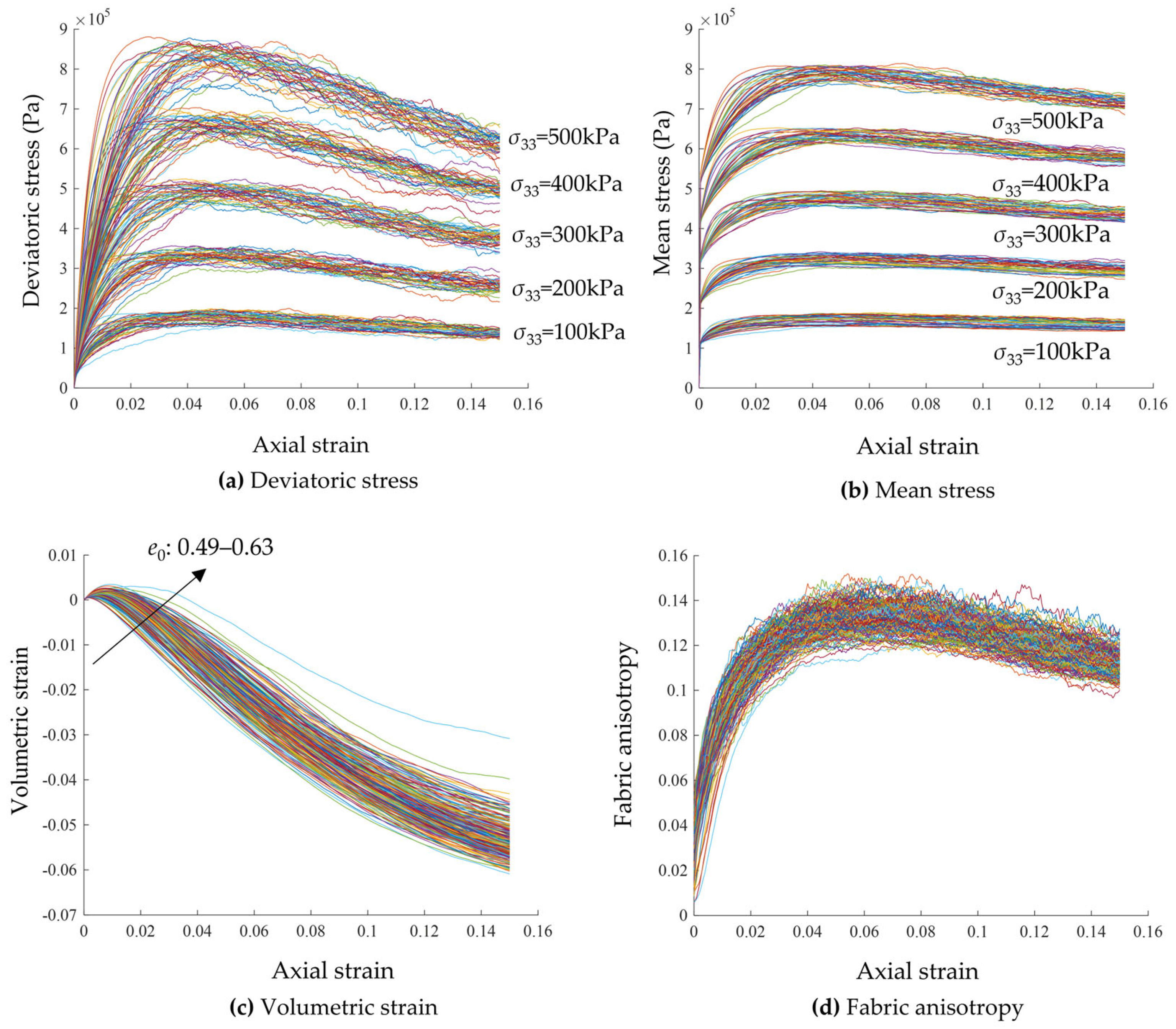
Figure 3 provides an overview of the full database of 200 DEM triaxial simulations assembled from controlled initial conditions. The PSD is characterized by Cu and d50, while the initial void ratio, initial fabric anisotropy, and confining pressure (100–500 kPa) are varied concurrently. Previous research has noted that the fabric anisotropy plays a critical role in the constitutive behaviour of granular soils [26,37,38]. It should be noted that the three-dimensional (3D) rose diagrams were commonly used to evaluate the directional fabric of the granular sample and its evolutionary process under loading by calculating the number of contacts falling within equally spaced patches [26]. Fabric anisotropy is superior to the traditional fabric tensor method due to its simpler calculation and lower data storage requirements. To describe the fabric anisotropy in a simple way, the standard deviation equation considering the variance of contact frequency was introduced to measure the fabric anisotropy as follows:
σ c 2 = i = 1 N ( x i μ ) 2 N ,
where σc stands for the standard deviation of the contribution for contact frequency; xi is the number of contacts falling within equally spaced patches; µ represents the average value of the contact frequency; and N is the number of patches equal to 320 in this study, striking a balance between computational efficiency and precision for characterizing the contact orientation distribution using 3D rose diagrams. Accordingly, the initial fabric anisotropy, denoted as σc0, was also quantified as a key input packing state variable in this study. The stress and strain variables are as follows:
p = σ 11 + 2 σ 33 3 ,
q = σ 11 σ 33 ,
ε v = Δ V V s ,
where σ 11 is the axial stress; σ 33 is the lateral stress; and V s and Δ V are the total sample volume and the change in sample volume, respectively.
Figure 3a,b present the evolutions of mean stress p and deviatoric stress q, respectively, under confining pressures varying between 100 and 500 kPa. The stress–strain curves are naturally divided into five unique scopes, featuring corresponding peak values of p and q in each range immensely affected by confining stress. Notably, with the increase in confining stress ranging from 100 to 500 kPa, the initial rate of rise and monolithic value of the stress–strain curves exhibit pronounced disparate distribution intervals appearing at a peak point within the range of 150 kPa to 860 kPa, respectively, which is accompanied by a visible phenomenon exhibiting different degrees of strain softening, concerning the initial void ratio, for the selected dense and medium dense granular samples particularly, as well as PSD-related parameters. Additionally, Figure 3c shows the volumetric strain vs. axial strain curves. It is obvious that both dense and medium dense samples undergo varying degrees of compression in the beginning and then convert into volumetric expansion. However, the mechanical behaviour is more intuitive in the dense sample, which presents a higher initial shear modulus and more pronounced behaviour of dilatancy compared to the medium dense one. The fabric anisotropy curves shown in Figure 3d display a relatively consistent pattern regardless of the initial void ratio and confining pressure, which features a monotonic increase up to a peak value within the range of 0.12–0.15 at around 4% to 6% strain and a subsequent gradual decrease to the range of 0.1–0.14 until the end of simulation. Notably, the representative comparisons between DEM simulations and ML predictive targets are selected from the 200 DEM specimens assembled from these controlled initial conditions. They are intended to span the PSD and initial-condition ranges and are depicted in the training, validation, and testing subsets to demonstrate the ML-based model’s reliability across diversity phases, rather than to represent a single “average-PSD” case.

3. Recurrent Neural Networks

3.1. LSTM-NN

Compared to the frequently used feed-forward neural networks, RNNs can connect input data at different time steps and are well-suited for solving sequential problems [39,40]. The key to determining the influence of previous loading history lies in the setting of the specific hyperparameter of the time step, which defines the extent of historical information affecting the current state. However, traditional RNNs may encounter vanishing or exploding gradient problems during the back-propagation process when dealing with long sequential problems, making it challenging to capture well the loading history-dependent constitutive behaviour of idealized granular materials. To address this issue, an LSTM-NN was introduced, which was used in a previous study to capture the constitutive response of quartz sand [39].
Figure 4 illustrates the schematic diagram and simplified structure of the LSTM-NN architecture to make the LSTM’s functionality more comprehensible. The workflow includes two state elements: a cell state for the long-term memory and a hidden state for the short-term memory. Moreover, a time-dependent LSTM-NN cell comprises three gates, namely, input gate, forget gate, and output gate. These gates are crucial for receiving new and historical information and producing output results.
The following steps describe the procedure of the LSTM-NN cell operation. Firstly, the input sequence at time step t is denoted as xt, and the value of the hidden state of the previous time step is denoted as ht−1. This means that the output at any given time step t is influenced not only by the current input state but also by the cumulative history of all past loading events. This characteristic is essential for accurately modeling loading history-dependent problems in granular materials. The forget gate determines what information will be discarded by taking the input values of xt and ht−1 into account and converting the output to the range from zero to one, representing a complete abandonment and reservation of the information, respectively. Then, the cell state is updated by combining the information from the input gate and the forget gate and feeding in a hyperbolic tangent function. Finally, the filtered output values are obtained through element-wise multiplication and addition, respectively. The output values of the input gate and the forget gate can be calculated using the following equations:
i t = σ W i h t 1 , x t + b i ,
f t = σ W f h t 1 , x t + b f ,
where h t 1 , x t denotes the concatenation of two inputs; W i and W f represent the weight matrices for the input and forget gates, respectively; b i and b f represent their corresponding bias vectors; and σ is the sigmoid function, which squeezes the output values into the range of zero and one.
The symbols C t and C t ~ are used to represent the cell state and the candidate cell state at the time step t, respectively. The candidate value can be formulated as follows:
C t ~ = tanh W C h t 1 , x t + b C ,
where W C and b C are the weight matrix and bias vector for the cell state, respectively; the activation function is the hyperbolic tangent function denoted as tanh.
Thus, the cell state can be calculated as follows:
C t = i t C t ~ + f t C t 1 ,
where denotes the element-wise multiplication. The first part of the element-wise product between i t and C t ~ signifies the information to be inputted to the cell state at time step t, while the second part of the element-wise product between f t and C t 1 represents the fraction to be retained in the cell state at the previous time step t−1. Subsequently, integrating these two components of the output values through element-wise addition is crucial for achieving a successful update of the cell state.
Next, a similar linear calculation is also applied to determine the values of the output gate. The formula is expressed as follow:
o t = σ W o h t 1 , x t + b o ,
where o t denotes the output gate vector at time step t; W o and b o are the weight matrix and bias vector for the output gate, respectively.
The output of the hidden state is the cell state processed by the activation function and the output gate, which is described as follows:
h t = o t tanh C t ,
where h t denotes the hidden state. As illustrated in Figure 4, the hidden state of the LSTM-NN is utilized as both a component of the output sequence and one of the crucial input parameters for the subsequent LSTM-NN cell.

3.2. GRU-NN

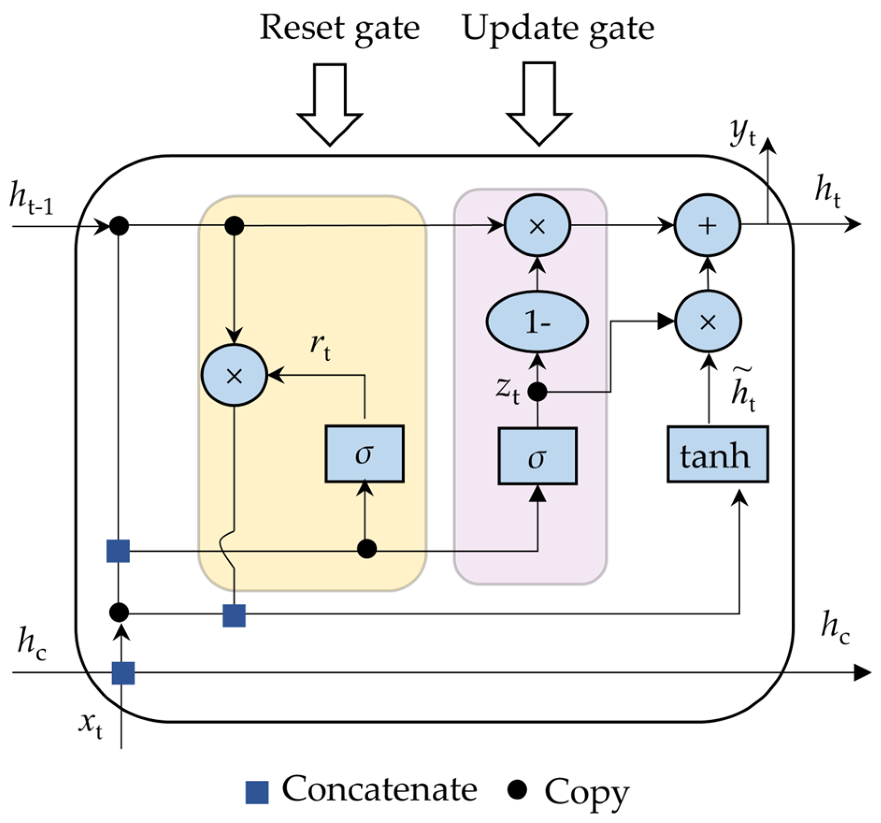
The GRU-NN proposed by Chung et al. [41] is a modified version of LSTM-NN that simplifies the architecture by reducing the number of gates from three to two. Specifically, the input gate and forget gate in LSTM-NN are merged into a single update gate in GRU-NN, while the cell state and hidden state are merged into a single hidden state. Despite its simpler structure, GRU-NN achieves a comparable performance to LSTM-NN in many applications [42,43]. Moreover, GRU-NN is superior in the aspects of computational efficiency and training duration in terms of requiring fewer parameters and experiencing fewer cell units during training. Figure 5 shows the schematic diagram of a typical GRU-NN architecture.
Similar to the LSTM-NN architecture, the GRU-NN architecture incorporates gating mechanisms that are closely linked to the concatenation of the input at the current time step and the hidden state at the previous time step. Specifically, GRU-NN employs an update gate and a reset gate in a highly effective way by adopting the following mathematical expressions:
z t = σ W z h t 1 , x t + b z ,
r t = σ W r h t 1 , x t + b r ,
where z t and r t are the outputs of the update gate and reset gate, respectively; W z and W r are their weight matrices; and b z and b r are their bias vectors. The outputs of these gates remain in the range of zero and one.
Next, the candidate hidden state is calculated as follows:
h t ~ = tanh W h r t h t 1 , x t + b h ,
where h t ~ denotes the candidate hidden state; W h and b h are the corresponding weight and bias vectors. It should be noted that in the GRU-NN architecture, if the reset gate converges to zero, the model will discard the information contained in the previous hidden state and rely solely on the input at the current time step. Conversely, when the reset gate approaches one, the recorded information is considered valuable and will integrate with the current information in the hidden state. This gating mechanism allows GRU-NN to selectively store and update information, depending on its relevance to the task at hand, and facilitates the capture of long-term dependencies in sequential data.
Overall, the final output of the GRU-NN cell, i.e., the new hidden state, is given by the following:
h t = z t h t ~ + 1 z t h t 1 ,
where h t represents the new hidden state. It can be seen that the update gate regulates the amount of new information that is stored in the hidden state, and also determines the degree to which the historical information should be retained or discarded.

3.3. Neural Network Architectures

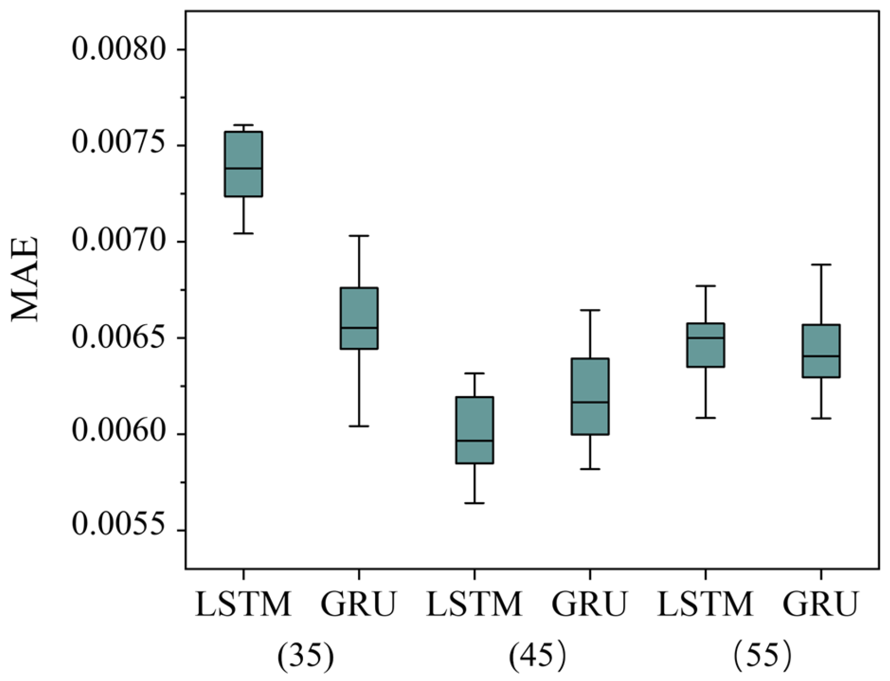
In this study, the dataset derived from DEM simulations was randomly divided into training (70%), validation (15%), and testing (15%) subsets for developing and evaluating the LSTM-NN and GRU-NN models. Specifically, the input parameters contain four initial packing state parameters (i.e., e, σc0, d50, and Cu), along with two mechanical state parameters (i.e., σ33 and ε1), while the four target sequence output variables are the deviatoric stress q-ε1, mean stress p-ε1, volumetric strain εv1, and fabric anisotropy σc1. A sliding window approach was employed to facilitate sequence-to-sequence learning for modeling the constitutive behavior of granular soils, thereby incorporating the history-dependent nature of granular materials into machine learning [6]. To ascertain the most effective sliding window size, different sliding window sizes of 35, 45, and 55 were tested herein. We employed the mean absolute error (MAE) as an error indicator to evaluate the model’s performance. The MAE is calculated using the formula M A E = i = 1 n | y ^ i y i | / n , where y ^ i denotes the predicted value of the concerned variable; y i denotes the actual value of the concerned variable; and n denotes the number of data point. The error values of the MAE associated with different sliding window sizes are shown in Figure 6.
It is evident from Figure 6 that the MAE values for both LSTM-NN and GRU-NN from the sliding window size of 45 are lowest. Accordingly, each sequence was partitioned into 256 overlapping sub-sequences (indexed from 0 to 255) with a fixed sliding window size of 45, which was shown to achieve the best trade-off between prediction accuracy and model robustness.
The configuration details of LSTM-NN and GRU-NN utilized in this study are presented in Table 4. Each model includes one sequence input layer, one regression output layer, and a single LSTM-NN or GRU-NN layer, followed by a fully connected layer, and was performed using the TensorFlow 2.9.0 platform. Specifically, the fully connected layer in LSTM-NN or GRU-NN is responsible for processing the output of the LSTM-NN or GRU-NN units and making a final prediction based on the sequence of inputs. Furthermore, the layer of LSTM or GRU is utilized to capture high-dimensional database features. When feeding the simulation data into LSTM-NN and GRU-NN, we implement a random seed setting, which ensures that the group-based data are input in a fixed sequence. This randomized sequence is crucial for training and testing ML models, which helps with preventing the models from developing biases or overfitting to a specific order of data presentation. These layers take the output of the LSTM-NN or GRU-NN units which is a sequence of hidden states as input and transform it into a fixed-length vector representation which can be used for the regression tasks. The hyperparameters including the number of hidden layer nodes, learning rate, epoch, loss function, optimizer and batch size are adjusted in the TensorFlow platform through a trial-and-error procedure to achieve the optimal performance.
To ensure that the entire dataset can be used for training, validating, and testing, we chose a batch size of 301, considering the number of records in each DEM simulation, along with computational efficiency and prediction accuracy. This specific value was selected to optimize the performance of our proposed ML-based models. An ‘epoch’ in ML, refers to one complete pass throughout the entire training dataset. The number of hidden layer nodes for the LSTM layer and GRU layer was set to 50, respectively, and the number of nodes for the fully connected layer was set to four. During an epoch, the model processes and learns from each sample in the training dataset once. The number of epoch and learning rate are fixed at 250 and 0.001, respectively, which was shown by our previous studies [26,39] to achieve the optimal solution and good convergence. The loss function is adopted to assess the performance of the algorithm and the adaptive moment estimation (Adam) optimizer is employed to accelerate the data fitting.
The nonlinear constitutive behaviour of granular materials is typically modelled through regression, for which the mean square error (MSE) is commonly employed as the loss function. The MSE is defined as follows:
M S E = 1 n i = 1 n ( y ^ i y i ) 2 ,
In addition to the MSE, the mean absolute percentage error (MAPE) and R-square, expressed by Equations (16) and (17) are adopted to evaluate the model performance in the testing stage. Generally, for MAPE and MSE, a lower value denotes a better performance, while a higher value indicates a better performance for R-square [22].
M A P E = 100 % n i = 1 n y ^ i y i y i ,
R s q u a r e = i = 1 n ( y ^ i y ¯ i ) 2 i = 1 n ( y i y ¯ i ) 2
where y ^ i denotes the predicted value of the concerned variable; y i denotes the actual value of the concerned variable; y ¯ i represents the average value of the actual value; and n denotes the number of data.
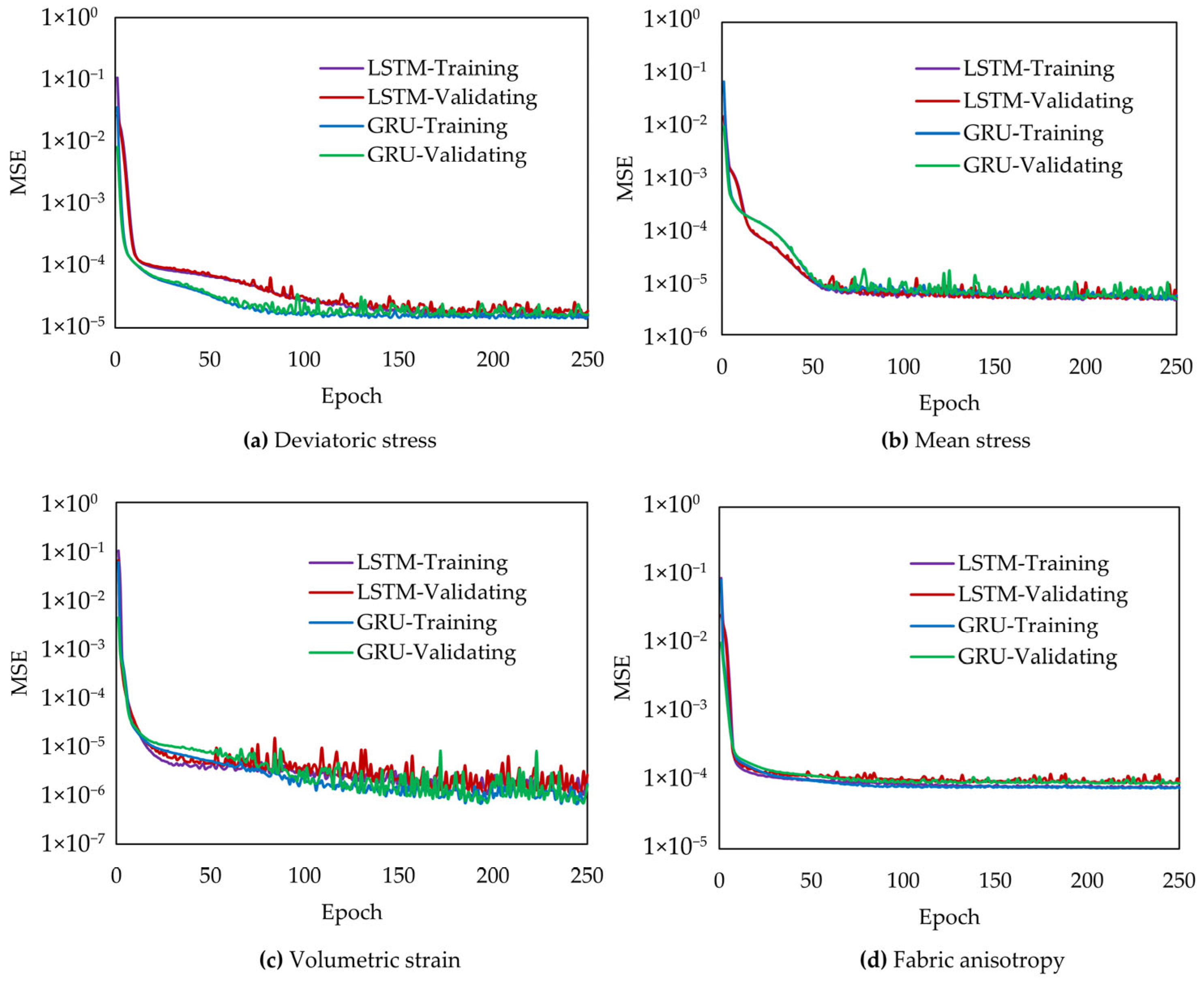
Figure 7 shows the evolution of the MSEs of the fabric anisotropy σc (Equation (1)), volumetric strain εv (Equation (4)), deviatoric stress q (Equation (3)), and mean stress p (Equation (2)) during the training and validating stages of the LSTM-NN and GRU-NN models. In this study, the DEM-derived database was randomly split into three subsets. Specifically, 70% of the dataset was allocated for regulating ML-based models’ trainable parameters in the training set, while 15% for validation was employed to evaluate the ML-based models’ performance on independent data at each training epoch without participating in backpropagation, thereby mitigating overfitting risks, as well as facilitating the hyperparameter tuning process (e.g., learning rate, batch size, optimizer, activation function, and network architecture).
A decreasing MSE value is a positive indicator, showing that the model can accurately predict outcomes even for data it has not been trained on. Additionally, for enhanced analysis, the curves can be divided into two parts. In the first part (Epoch 0–20), a sharp decrease in MSE values for both LSTM-NN and GRU-NN is observed, indicating that both networks can effectively capture the mechanical behaviours of idealized granular soils. The curve of GRU-NN appears to have an earlier turning point and lower values than that of LSTM-NN under certain conditions, indicating that GRU-NN achieves a comparable performance to LSTM-NN to some extent. Meanwhile, in the second phase of the training and validating process (Epoch 21–250), both LSTM-NN and GRU-NN exhibit a decreased rate of decline for their MSE values with varying degrees of fluctuation. Comparing the results of both models, the MSE values for LSTM-NN represent a higher and less stable error standard than GRU-NN for capturing deviatoric stress and fabric anisotropy.

4. Results

4.1. Training, Validating, and Testing Results

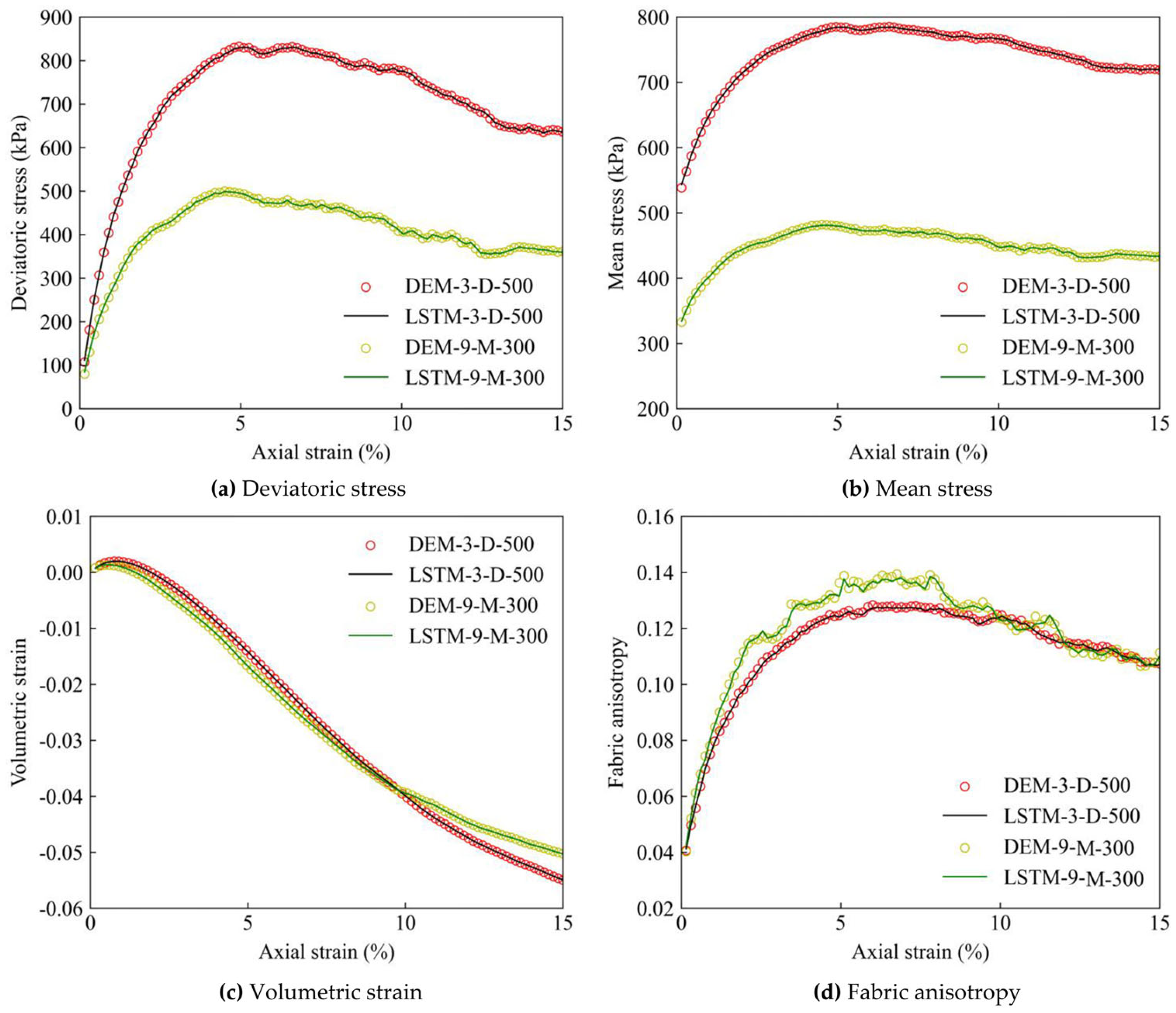
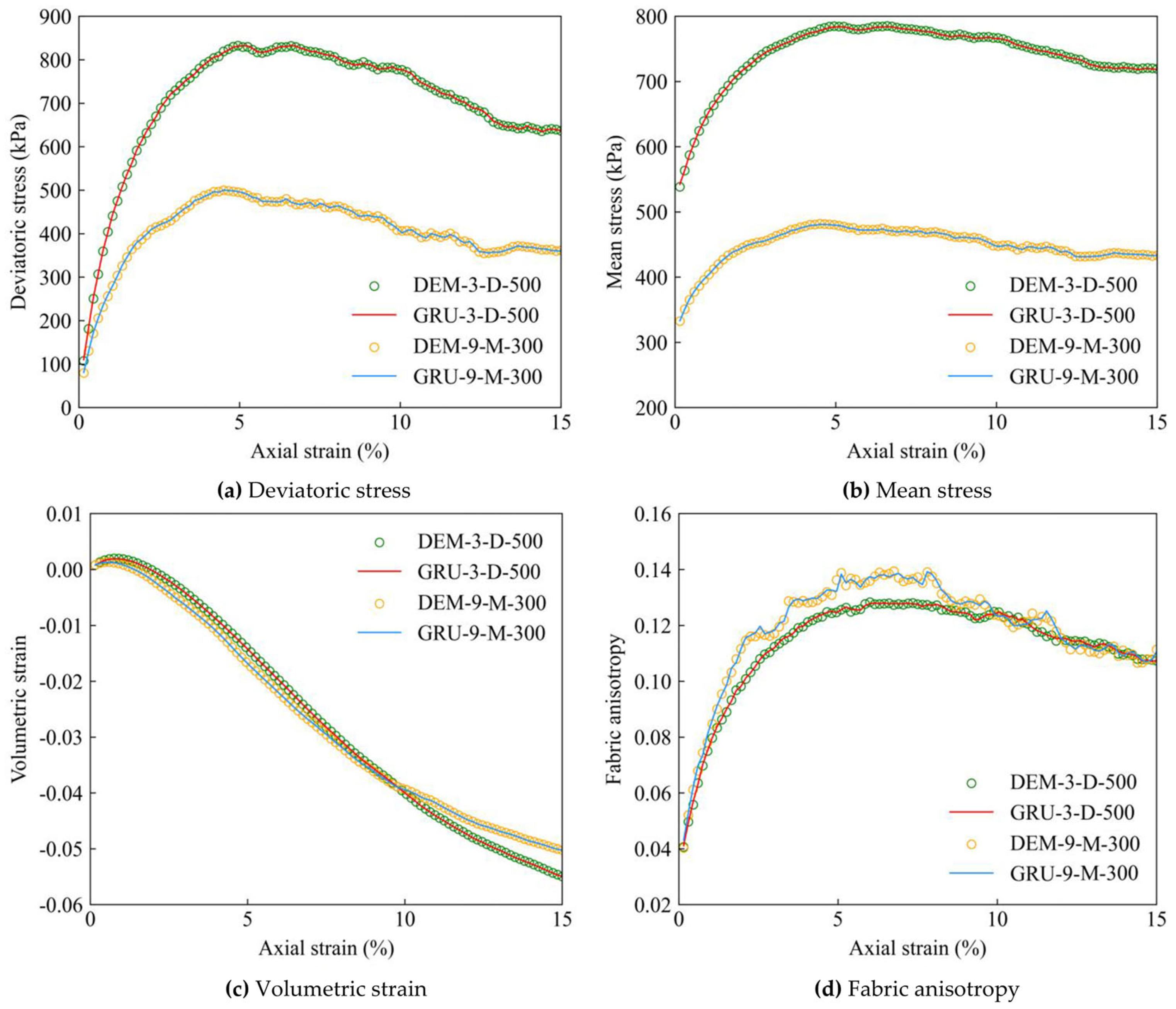
Figure 8 and Figure 9 present the training results of LSTM-NN and GRU-NN for predicting the relationship between p, q, εv, σc, and ε1. The curves are denoted by a code with a format of ‘DEM/LSTM/GRU-a-D/M-b’, in which the approach used is represented by either DEM, LSTM, or GRU, ‘a’ represents the ID of the particle size template, ‘D’ or ‘M’ denotes the type of sample, either dense or medium dense, and ‘b’ represents the confining pressure. Each input sub-sequence and its next-step targets form a training sample, enabling the ML-based modeling to learn the loading history dependency of the mechanical responses of the granular samples. It is observed that during the training process, the predictions of both ML-based models closely match the DEM simulation data for all target variables. These results show the strong capability of ML-based models in learning the macro and micro mechanical behaviours of granular soils.
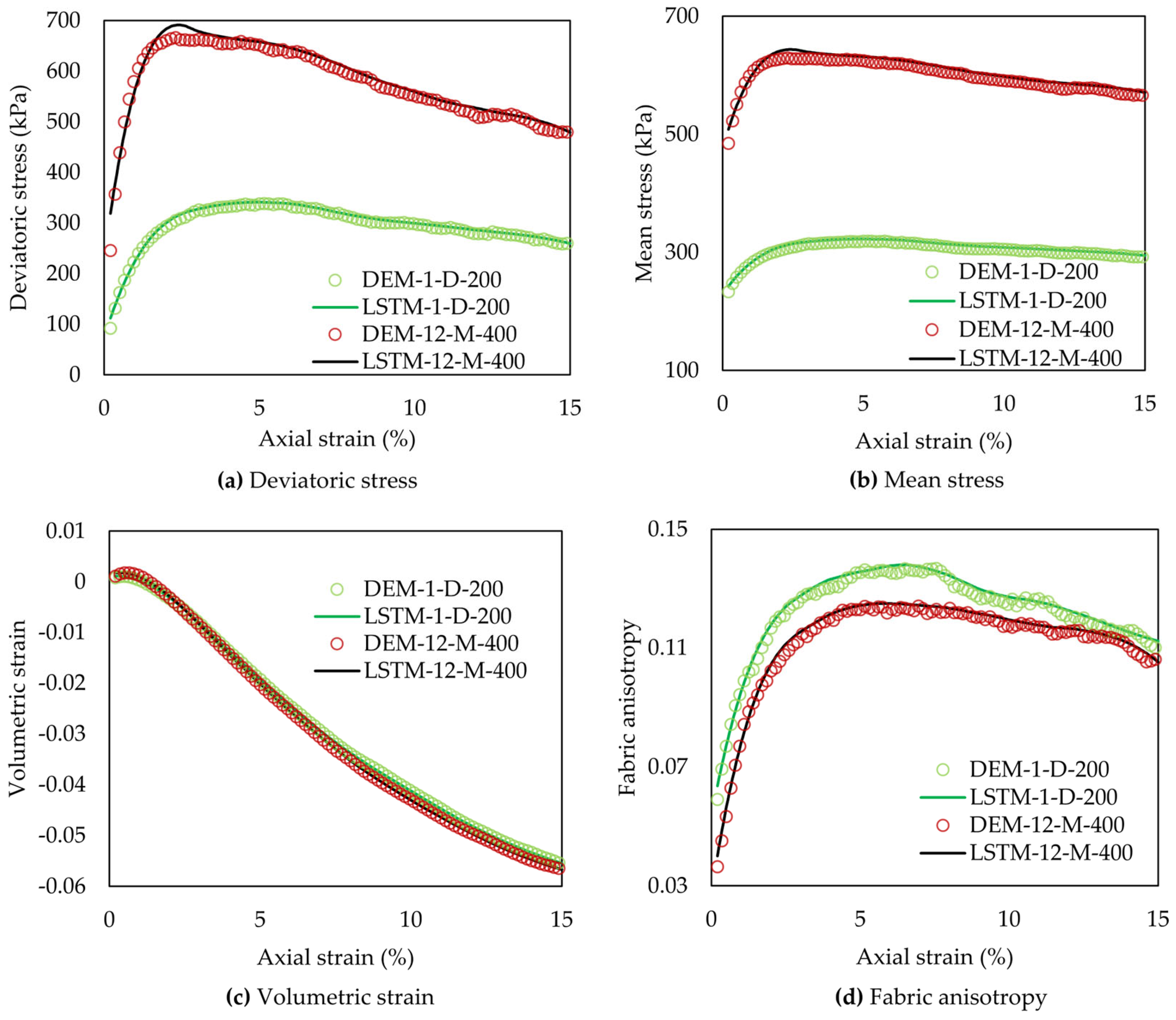
Figure 10 and Figure 11 clearly show a close agreement between the results of LSTM-NN or GRU-NN and DEM simulations for the validation cases. The well-trained models are evaluated on the 15% unseen sequential data using the sliding window approach, where predictions are generated and updated iteratively along the full mechanical response trajectory through forward propagation exclusively. The results demonstrate that the proposed ML-based models accurately predict the complex constitutive behavior of granular soils across both macroscopic and microscopic responses.
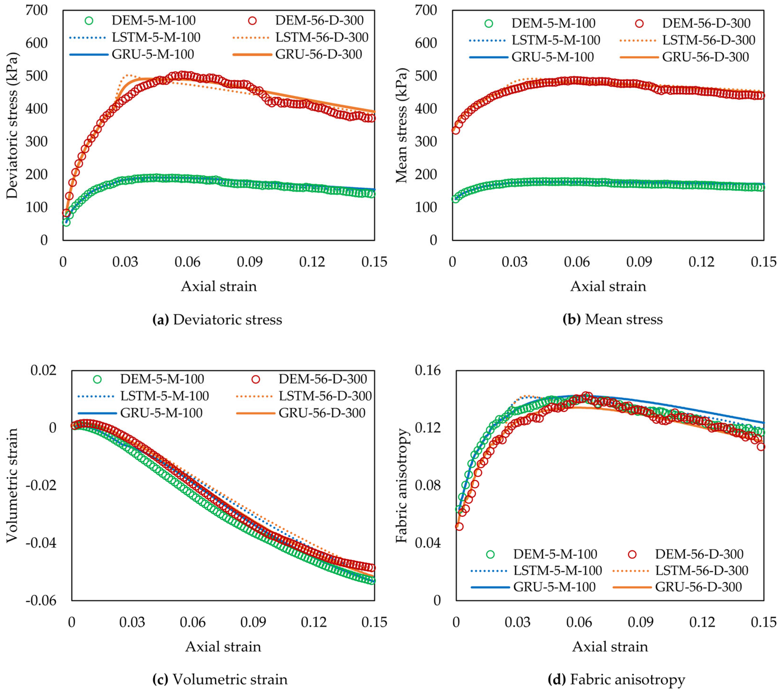
Figure 12 presents a comparative evaluation of the predictive performance between LSTM-NN and GRU-NN models against DEM simulation results. During the testing phase, the first 45 pairs of consecutive variables, in terms of input features and corresponding history-dependent output variables, were used to initialize the first sliding slices. Thereafter, the ML-based models generated predictions in an autoregressive manner, whereby the predicted outputs from previous time steps were iteratively performed as inputs for predicting subsequent responses. This strategy enabled the model to predict the entire response trajectory without the need for additional ground-truth outputs beyond the initial sliding slices.
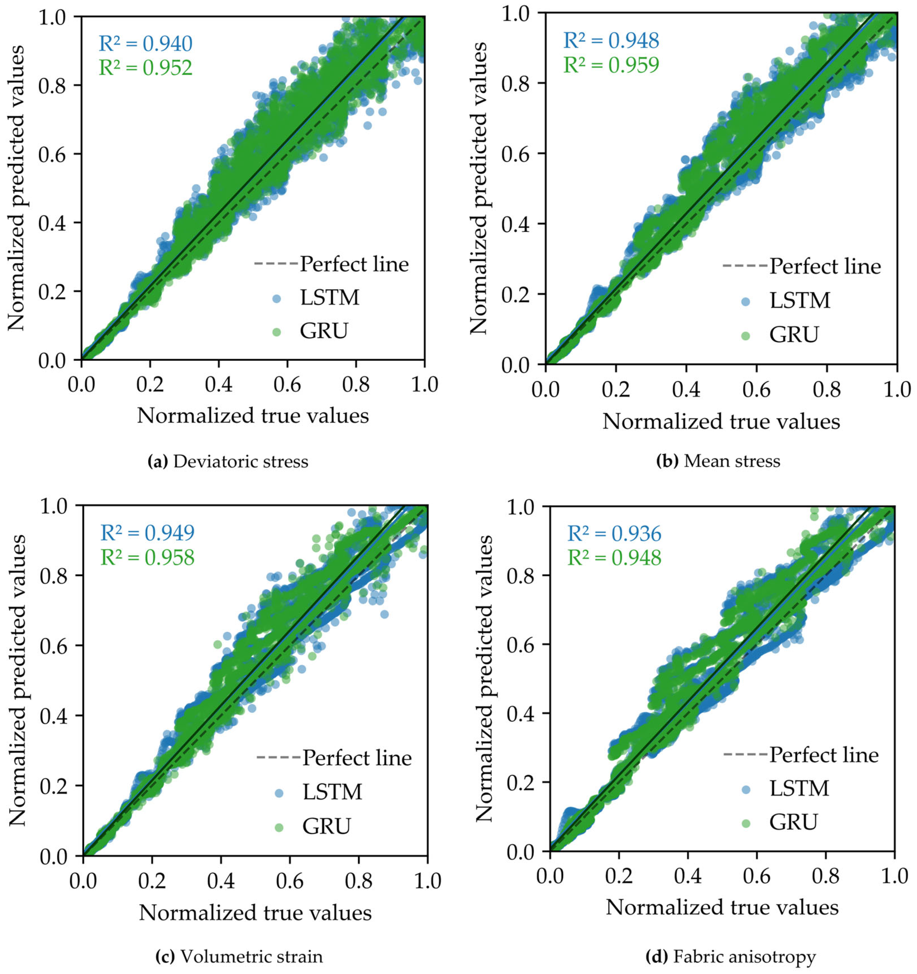
Figure 13 and Figure 14 present the box plots of MAPE and R-square for all of the testing datasets. The red horizontal lines represent the mean values of MAPE and satisfactory value of R-square, which signifies the overall performance of the LSTM-NN and GRU-NN. The maroon boxes represent the main error ranges of MAPE for all variables, while the top and bottom scale bar denote the maximum and minimum values of MAPE, respectively. It is found that the MAPE values of all modelled variables from the testing datasets are around 0.2%, while R-square is larger than 0.94, except for the fabric anisotropy, whose MAPE values are approximately 0.5%, with R-square = 0.936 and 0.948 for the LSTM-NN and GRU-NN, respectively, which displays a generally worse prediction with higher error than the other three variables. This result suggests that the fabric anisotropy becomes more oscillatory when the sample reaches the critical state, which agrees well with the observation made by Wu et al. [26].

4.2. Application of ML-Based Models to Micro-CT Triaxial Test

It will be desirable to apply the trained LSTM-NN and GRU-NN to predict the constitutive behaviour of a miniature spherical glass bead sample subjected to triaxial shearing, as observed in the micro-CT tests by Cheng and Wang [44]. We gathered all essential initial variables necessary for the ML-based model prediction from Cheng and Wang [44]. These input data encompassed parameters such as the initial void ratio, initial fabric, particle size distribution (PSD) characteristics, and the evolution of key variables like deviatoric stress, mean stress, volumetric strain, and fabric anisotropy in relation to axial strain. Specifically, for the glass bead sample, the input parameters were as follows: mean particle size = 0.4 mm, uniformity coefficient = 1.29, initial void ratio = 0.49, initial fabric = 0.003, and confining pressure = 500 kPa. It should be noted that the DEM simulations have been thoughtfully set up to mimic the micro-CT test by adopting a set of DEM models and material properties that are very close to those of the physical test, including the simplified spherical particle shapes and similar sample dimensions, particle size distribution (PSD) characteristics, and loading rates.
Figure 15 compares the predictions of the LSTM-NN and GRU-NN with the micro-CT test results. It is observed that an overall good agreement exists between the ML predictions and experimental results. The sliding window size critically governs the long-sequence prediction accuracy of LSTM and GRU networks. A shorter window size restricts the historical information contained in each sub-sequence, thereby constraining the prediction accuracy to capture long-term dependencies for ML modeling [6]. Furthermore, the initial 45 pairs of consecutive history-dependent output variables are progressively replaced by the predicted values along the full trajectory. This substitution contributes to error accumulation, as the discrepancy between predicted and true values amplifies with each sliding step. This feature differs from the ML-based model prediction of the micro-CT test in our previous studies [22,39], which is mainly responsible for the deviations of the model prediction from the experimental results. In addition, a slight tilting of the upper loading platen of the glass bead specimen was observed in the micro-CT test, which promotes the slightly higher degrees of shear localization and the overall specimen distortion of the specimen deformation [45], leading to a differentiated development trend between experiments and ML predictions.

4.3. Generalization Capability of ML-Based Models

To further investigate the generalization ability of the developed ML models, two additional DEM simulations, namely, Test Set 201 and 202 with a mean particle size of 0.2 mm and 0.6 mm, a uniformity coefficient of five, an initial fabric of 0.021 and 0.038, an initial void ratio of 0.53 and 0.68, and a confining pressure of 550 kPa and 500 kPa, respectively, were performed. Note that the values of mean particle size, initial void ratio, and confining pressure are not covered by the range of the training dataset.
Figure 16 and Figure 17 compare the predictive constitutive responses from LSTM-NN and GRU-NN with DEM simulation results for Test Set 201 and 202, respectively. Notably, the predicted curves of p, q, εv, and σc from both ML models basically confirm the DEM results. It is believed that both the LSTM-NN and GRU-NN possess the capability to capture the mechanical responses at a larger range of initial void ratio than 0.49–0.63 and confining pressure of 100–500 kPa, due to their proficiency in handling time sequence data with the sliding window approach. Inevitably, the error accumulation between predicted and true values still remains with each sliding step. In comparison, it is found that GRU-NN slightly outperforms LSTM-NN in fitting εv in the above strain range. The above results clearly demonstrate that both ML models have very good extrapolation capabilities within the range of the testing dataset. Nevertheless, a more comprehensive investigation of the ML model’s generalization capability needs to be carried out in our future study.

5. Concluding Remarks

In this study, a data-driven framework was developed for the constitutive modelling of granular soils. Two loading history-dependent algorithms, namely the LSTM-NN and GRU-NN, were employed to learn and predict the constitutive behaviours of idealized granular media directly from a DEM-generated dataset. For each simulation, 301 sequential data points were extracted, capturing key mechanical responses including deviatoric stress, mean stress, volumetric strain, and fabric anisotropy, while the influential factors, such as mean particle size, uniformity coefficient, initial fabric anisotropy, initial void ratio, confining pressure, and axial strain, served as the input parameters. To handle the normalized pairs of sequential data containing historical information, a sliding window strategy was adopted to iteratively forecast the full stress–strain trajectory.
The performance of the ML-based models was quantitatively evaluated by comparing their predictions with DEM simulation data. The test results indicate that the well-trained models accurately capture the constitutive behaviors across the whole range of axial strain, regardless of the initial packing state and stress conditions. Moreover, the reasonable predictive results of the μCT experiment and the two extrapolated test sets demonstrate that the proposed data-driven approach, which requires a short warm-up sequence of output variables as historical inputs, achieves a strong long-sequence forecasting performance and exhibits a robust generalization capability and reliability.
The comparison of the two neural network models reveals that the GRU-NN outperforms the LSTM-NN in terms of structure optimization, prediction accuracy, computational efficiency, and extrapolated analysis within the proposed data-driven framework. This advantage likely stems from the GRU’s simpler gating and fewer trainable parameters, enabling easier and more stable optimization and training. This multiscale framework offers high flexibility, as the well-trained models can be efficiently fine-tuned when additional data become available. In the future, we aim to develop a more comprehensive, nuanced constitutive model for granular soils that accounts for stress-path effects, realistic particle shapes, cyclic loading, particle crushing, etc., and implement such data-driven models in the FEM simulation to address large-scale boundary value problems in geotechnical engineering.

Author Contributions

Conceptualization, J.W.; Data curation, X.L.; Formal analysis, X.L.; Funding acquisition, J.W.; Investigation, X.L.; Methodology, X.L.; Project administration, J.W.; Resources, J.W.; Software, X.L.; Supervision, J.W.; Validation, X.L.; Visualization, X.L.; Writing—original draft, X.L.; Writing—review and editing, J.W. All authors have read and agreed to the published version of the manuscript.

Funding

This study was supported by the General Research Fund No. CityU 11204224 and No. CityU 11207321 from the Research Grants Council of the Hong Kong SAR, and Research Grant No. 52378371 from the National Science Foundation of China.

Data Availability Statement

The original contributions presented in this study are included in the article. Further inquiries can be directed to the corresponding author.

Acknowledgments

The authors acknowledge the help and support from the BL13W beam-line of the Shanghai Synchrotron Radiation Facility (SSRF).

Conflicts of Interest

The authors declare no conflicts of interest.

References

  1. Cerato, A.B.; Lutenegger, A.J. Scale effects of shallow foundation bearing capacity on granular material. J. Geotech. Geoenviron. Eng. 2007, 133, 1192–1202. [Google Scholar] [CrossRef]
  2. Li, M.; Fannin, R.J. Comparison of two criteria for internal stability of granular soil. Can. Geotech. J. 2008, 45, 1303–1309. [Google Scholar] [CrossRef]
  3. Das, B.; Sivakugan, N. Settlements of shallow foundations on granular soil—An overview. Int. J. Geotech. Eng. 2007, 1, 19–29. [Google Scholar] [CrossRef]
  4. Hungr, O. Simplified models of spreading flow of dry granular material. Can. Geotech. J. 2008, 45, 1156–1168. [Google Scholar] [CrossRef]
  5. Moraci, N.; Mandaglio, M.C.; Ielo, D. Analysis of the internal stability of granular soils using different methods. Can. Geotech. J. 2014, 51, 1063–1072. [Google Scholar] [CrossRef]
  6. Ma, G.; Guan, S.; Wang, Q.; Feng, Y.T.; Zhou, W. A predictive deep learning framework for path-dependent mechanical behavior of granular materials. Acta Geotech. 2022, 17, 3463–3478. [Google Scholar] [CrossRef]
  7. Qu, T.; Di, S.; Feng, Y.T.; Wang, M.; Zhao, T.; Wang, M. Deep learning predicts stress–strain relations of granular materials based on triaxial testing data. Comput. Model. Eng. Sci. 2021, 128, 129–144. [Google Scholar] [CrossRef]
  8. Jiang, M.J. New paradigm for modern soil mechanics: Geomechanics from micro to macro. Chin. J. Geotech. Eng. 2019, 41, 195–254. [Google Scholar]
  9. Tien Bui, D.; Hoang, N.D.; Nhu, V.H. A swarm intelligence-based machine learning approach for predicting soil shear strength for road construction: A case study at Trung Luong National Expressway Project (Vietnam). Eng. Comput. 2019, 35, 955–965. [Google Scholar] [CrossRef]
  10. Hashemi Jokar, M.; Mirasi, S. Using adaptive neuro-fuzzy inference system for modeling unsaturated soils shear strength. Soft Comput. 2018, 22, 4493–4510. [Google Scholar] [CrossRef]
  11. Abozraig, M.; Ok, B.; Yildiz, A. Determination of shear strength of coarse-grained soils based on their index properties: A comparison between different statistical approaches. Arab. J. Geosci. 2022, 15, 593. [Google Scholar] [CrossRef]
  12. Zhang, P.; Yin, Z.Y.; Jin, Y.F. An AI-based model for describing cyclic characteristics of granular materials. Int. J. Numer. Anal. Methods Geomech. 2020, 44, 1315–1335. [Google Scholar] [CrossRef]
  13. Cubuk, E.D.; Schoenholz, S.S.; Rieser, J.M.; Malone, B.D.; Rottler, J.; Durian, D.J.; Kaxiras, E.; Liu, A.J. Identifying structural flow defects in disordered solids using machine-learning methods. Phys. Rev. Lett. 2015, 114, 108001. [Google Scholar] [CrossRef] [PubMed]
  14. Rouet-Leduc, B.; Hulbert, C.; Bolton, D.C.; Ren, C.X.; Riviere, J.; Marone, C.; Guyer, R.A.; Johnson, P.A. Estimating fault friction from seismic signals in the laboratory. Geophys. Res. Lett. 2018, 45, 1321–1329. [Google Scholar] [CrossRef]
  15. Zhang, P.; Jin, Y.F.; Yin, Z.Y. Machine learning-based uncertainty modelling of mechanical properties of soft clays relating to time-dependent behaviour and its application. Int. J. Numer. Anal. Methods Geomech. 2021, 45, 1588–1602. [Google Scholar] [CrossRef]
  16. Liu, X.; Li, Z.; Zou, D.; Sun, L.; Ebrahim, K.Y.; Liang, J. Improving the prediction accuracy of small-strain shear modulus of granular soils through PSD: An investigation enabled by DEM and machine learning technique. Comput. Geotech. 2023, 157, 105355. [Google Scholar] [CrossRef]
  17. El Shamy, U.; Abdelhamid, Y. Modeling granular soils liquefaction using coupled lattice Boltzmann method and discrete element method. Soil Dyn. Earthq. Eng. 2014, 67, 119–132. [Google Scholar] [CrossRef]
  18. Pistolesi, F.; Baldassini, M.; Volpe, E.; Focacci, F.; Cattoni, E. Fast and interpretable prediction of seismic kinematics of flexible retaining walls in sand through explainable artificial intelligence. Comput. Geotech. 2025, 179, 107007. [Google Scholar] [CrossRef]
  19. Gordan, B.; Jahed Armaghani, D.; Hajihassani, M.; Monjezi, M. Prediction of seismic slope stability through combination of particle swarm optimization and neural network. Eng. Comput. 2016, 32, 85–97. [Google Scholar] [CrossRef]
  20. Mustafa, M.R.; Rezaur, R.B.; Saiedi, S.; Rahardjo, H.; Isa, M.H. Evaluation of MLP-ANN training algorithms for modeling soil pore-water pressure responses to rainfall. J. Hydrol. Eng. 2012, 18, 50–57. [Google Scholar] [CrossRef]
  21. Kouadri, S.; Pande, C.B.; Panneerselvam, B.; Moharir, K.N.; Elbeltagi, A. Prediction of irrigation groundwater quality parameters using ANN, LSTM, and MLR models. Environ. Sci. Pollut. Res. 2022, 29, 21067–21091. [Google Scholar] [CrossRef]
  22. Liu, Y.; Li, M.; Su, P.; Ma, B.; You, Z. Porosity prediction of granular materials through discrete element method and back propagation neural network algorithm. Appl. Sci. 2020, 10, 1693. [Google Scholar] [CrossRef]
  23. Hochreiter, S.; Schmidhuber, J. Long short-term memory. Neural Comput. 1997, 9, 1735–1780. [Google Scholar] [CrossRef]
  24. Kawakami, K. Supervised Sequence Labelling with Recurrent Neural Networks. Ph.D. Thesis, Technical University of Munich, Munich, Germany, 2008. [Google Scholar]
  25. Cundall, P.A.; Strack, O.D. A discrete numerical model for granular assemblies. Géotechnique 1979, 29, 47–65. [Google Scholar] [CrossRef]
  26. Wu, M.; Xia, Z.; Wang, J. Constitutive modelling of idealised granular materials using machine learning method. J. Rock Mech. Geotech. Eng. 2023, 15, 1038–1051. [Google Scholar] [CrossRef]
  27. Li, G.X. Advanced Soil Mechanics; Tsinghua University Press: Beijing, China, 2004. [Google Scholar]
  28. Itasca Consulting Group Inc. PFC 6.0 Documentation; Itasca Consulting Group Inc.: Minneapolis, MN, USA, 2019. [Google Scholar]
  29. Thornton, C. Quasi-static simulations of compact polydisperse particle systems. Particuology 2010, 8, 119–126. [Google Scholar] [CrossRef]
  30. Das, S.K.; Das, A. Influence of quasi-static loading rates on crushable granular materials: A DEM analysis. Powder Technol. 2019, 344, 393–403. [Google Scholar] [CrossRef]
  31. Mindlin, R.D.; Deresiewicz, H. Elastic spheres in contact under varying oblique forces. J. Appl. Mech. 1953, 20, 327–344. [Google Scholar] [CrossRef]
  32. Somfai, E.; Roux, J.N.; Snoeijer, J.H.; Van Hecke, M.; Van Saarloos, W. Elastic wave propagation in confined granular systems. Phys. Rev. E 2005, 72, 021301. [Google Scholar] [CrossRef]
  33. De Bono, J.P.; McDowell, G.R. DEM of triaxial tests on crushable sand. Granul. Matter 2014, 16, 551–562. [Google Scholar] [CrossRef]
  34. He, H.; Senetakis, K.; Coop, M.R. An investigation of the effect of shearing velocity on the inter-particle behaviour of granular and composite materials with a new micromechanical dynamic testing apparatus. Tribol. Int. 2019, 134, 252–263. [Google Scholar] [CrossRef]
  35. Itasca Consulting Group Inc. PFC3D User’s Guide; Itasca Consulting Group Inc.: Minneapolis, MN, USA, 2008. [Google Scholar]
  36. Wu, M.; Wang, J.; Russell, A.; Cheng, Z. DEM modelling of mini-triaxial test based on one-to-one mapping of sand particles. Géotechnique 2021, 71, 714–727. [Google Scholar] [CrossRef]
  37. Thornton, C. Numerical simulations of deviatoric shear deformation of granular media. Géotechnique 2000, 50, 43–53. [Google Scholar] [CrossRef]
  38. Sitharam, T.G.; Dinesh, S.V.; Shimizu, N. Micromechanical modeling of monotonic drained and undrained shear behaviour of granular media using three-dimensional DEM. Int. J. Numer. Anal. Methods Geomech. 2002, 26, 1167–1189. [Google Scholar] [CrossRef]
  39. Wu, M.; Wang, J. Constitutive modelling of natural sands using a deep learning approach accounting for particle shape effects. Powder Technol. 2022, 404, 117439. [Google Scholar] [CrossRef]
  40. Qu, T.; Guan, S.; Feng, Y.T.; Ma, G.; Zhou, W.; Zhao, J. Deep active learning for constitutive modelling of granular materials: From representative volume elements to implicit finite element modelling. Int. J. Plast. 2023, 164, 103576. [Google Scholar] [CrossRef]
  41. Chung, J.; Gulcehre, C.; Cho, K.; Bengio, Y. Empirical evaluation of gated recurrent neural networks on sequence modelling. arXiv 2014, arXiv:1412.3555. [Google Scholar] [CrossRef]
  42. De Melo, G.A.; Sugimoto, D.N.; Tasinaffo, P.M.; Santos, A.H.M.; Cunha, A.M.; Dias, L.A.V. A new approach to river flow forecasting: LSTM and GRU multivariate models. IEEE Lat. Am. Trans. 2019, 17, 1978–1986. [Google Scholar] [CrossRef]
  43. Shewalkar, A.; Nyavanandi, D.; Ludwig, S.A. Performance evaluation of deep neural networks applied to speech recognition: RNN, LSTM and GRU. J. Artif. Intell. Soft Comput. Res. 2019, 9, 235–245. [Google Scholar] [CrossRef]
  44. Cheng, Z.; Wang, J. Experimental investigation of inter-particle contact evolution of sheared granular materials using X-ray micro-tomography. Soils Found. 2018, 58, 1492–1510. [Google Scholar] [CrossRef]
  45. Cheng, Z.; Wang, J.; Xiong, W. A machine learning-based strategy for experimentally estimating force chains of granular materials using X-ray micro-tomography. Géotechnique 2024, 74, 1291–1303. [Google Scholar] [CrossRef]
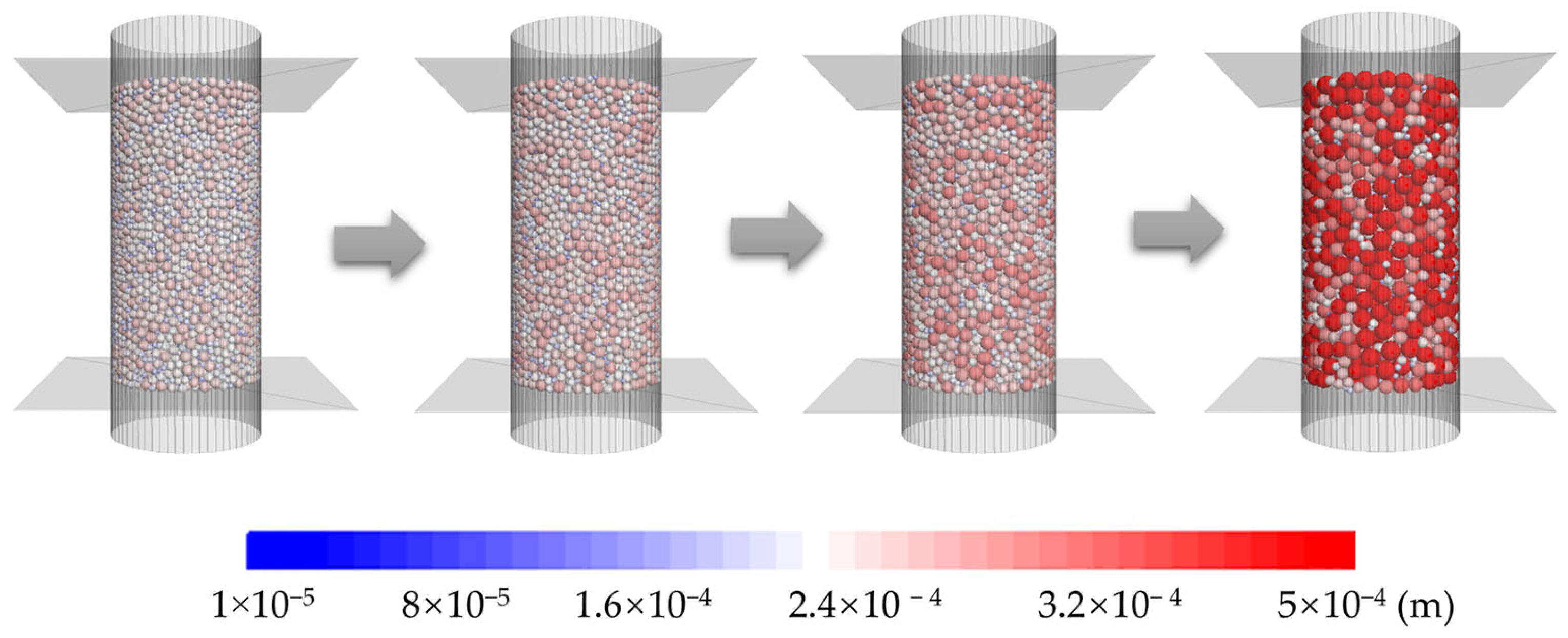
Figure 1. Particle size distributions used to generate the granular samples (the color bar indicates the distribution of the ball radius).
Applsci 15 09495 g001
Figure 2. Flowchart of the research methodology.
Applsci 15 09495 g002
Figure 3. DEM simulation results.
Applsci 15 09495 g003
Figure 4. Scheme diagram and simplified structure for LSTM-NN cell.
Applsci 15 09495 g004
Figure 5. Schematic diagram for GRU-NN cell.
Applsci 15 09495 g005
Figure 6. Influence of sliding window size for machine learning models.
Applsci 15 09495 g006
Figure 7. Evolutions of loss value using LSTM and GRU.
Applsci 15 09495 g007
Figure 8. Training results for the LSTM model.
Applsci 15 09495 g008
Figure 9. Training results for the GRU model.
Applsci 15 09495 g009
Figure 10. Validating results for the LSTM model.
Applsci 15 09495 g010
Figure 11. Validating results for the GRU model.
Applsci 15 09495 g011
Figure 12. Testing results for LSTM and GRU models.
Applsci 15 09495 g012
Figure 13. Testing performance of R-square for LSTM and the GRU.
Applsci 15 09495 g013
Figure 14. Mean absolute percentage error for the testing sets.
Applsci 15 09495 g014
Figure 15. Predicted constitutive relationships on the micro-CT experiment.
Applsci 15 09495 g015
Figure 16. Predicted constitutive relationships on Test Set 201 (extrapolation).
Applsci 15 09495 g016
Figure 17. Predicted constitutive relationships on Test Set 202 (extrapolation).
Applsci 15 09495 g017
Table 1. Main features of typical ML-based models.
ModelFeaturesDrawbacks
ANNSimplicity in structure
Computational efficiency
Interpretability
Single output prediction
Poor nonlinear mapping ability
BPNNNonlinear mapping ability
Multi-outputs prediction ability
Gradients exploding or vanishing
Limitations in time-related prediction
RNNSequential data prediction ability
Nonlinear mapping ability
Multi-outputs prediction ability
Gradients exploding or vanishing
Limitations in time-related prediction
LSTMSequential data prediction ability
Nonlinear mapping ability
Multi-outputs prediction ability
Numerous weights and biases and hyperparameters
GRUSequential data prediction ability
Nonlinear mapping ability
Multi-outputs prediction ability
Numerous weights and biases and hyperparameters
Table 2. Ranges of initial sample parameters in DEM simulations.
Twenty particle size distributions (d50/mm, Cu)(0.3, 4), (0.3, 4.5), (0.3, 5), (0.3, 5.5),
(0.35, 3), (0.35, 4), (0.35, 5.5), (0.35, 6),
(0.4, 2), (0.4, 3), (0.4, 4.5), (0.4, 5),
(0.45, 2), (0.45, 3), (0.45, 4), (0.45, 5),
(0.5, 4), (0.5, 4.5), (0.5, 5), (0.5, 5.5)
Five confining stresses, σ33 (kPa)100, 200, 300, 400, 500
Two void ratios, e0.49, 0.63
Total number of DEM simulations200
Table 3. The parameters utilized in numerical simulations.
ParametersValue
Contact modelHertz–Mindlin
Friction coefficient0.3
Wall friction coefficient0
Damping coefficient0.7
Shear modulus (GPa)28
Poisson’s ratio0.25
Density (kg/m3)2650
Size: height × diameter (mm)16 × 8
Table 4. The neural network structures.
Model IDLayer NameProjectNum. of NodesActivation FunctionNote
Model-1LSTM-NNCapturing high-dimensional features50ReLULearning rate = 0.001;
Epochs = 250;
Optimizer = Adam;
Loss function = MSE;
Batch size = 301
Fully connected layerDimensional transformation4Linear
Model-2GRU-NNCapturing high-dimensional features50ReLU
Fully connected layerDimensional transformation4Linear
Disclaimer/Publisher’s Note: The statements, opinions and data contained in all publications are solely those of the individual author(s) and contributor(s) and not of MDPI and/or the editor(s). MDPI and/or the editor(s) disclaim responsibility for any injury to people or property resulting from any ideas, methods, instructions or products referred to in the content.