Article

Three-Way Decision-Driven Adaptive Graph Convolution for Deep Clustering

1
School of Software Engineering, South China University of Technology, Guangzhou 510006, China
2
State Key Laboratory of Pulp and Paper Engineering, South China University of Technology, Guangzhou 510006, China
*
Author to whom correspondence should be addressed.
Appl. Sci. 2025, 15(17), 9391; https://doi.org/10.3390/app15179391
Submission received: 5 August 2025 / Revised: 20 August 2025 / Accepted: 23 August 2025 / Published: 27 August 2025
(This article belongs to the Section Computing and Artificial Intelligence)

Abstract

Graph clustering is an efficient method for deep clustering that utilizes graph convolution. Graph convolution effectively combines structure and content information, and lots of recent graph convolution-based methods have shown promising results in clustering performance on actual attribution networks. However, the established methods mainly employ a fixed graph convolution order, and limited studies have focused on the flexible choice of k-order graph convolution. When utilizing graph convolution with a fixed low order, only considering a few hops per node or neighbors within a set range of hops fails to maximize node relationships or account for the variations within the graphs. In this paper, we propose an adaptive method for graph clustering using a three-way decision idea. Our method enables the adaptive selection of k-order graph convolution for different graphs by searching for the k-order convolution kernel that best suits the subsequent clustering task. Additionally, our approach uses higher-order graph convolution to capture the global clustering structure. We assess the effectiveness of our approach through theoretical analysis and extensive experiments on benchmark datasets. Empirical evidence indicates that our method surpasses state-of-the-art techniques.

1. Introduction

Graph Convolutional Networks (GCNs) are powerful tools for learning representations from graph data. They have achieved remarkable success in many graph analysis tasks, especially in graph clustering [1,2]. GCNs work by aggregating information from a node’s neighbors [3]. This process effectively fuses the graph’s structural topology with its node attributes. The result is a high-quality feature representation that is well-suited for downstream clustering algorithms. However, the performance of a GCN is highly sensitive to its number of convolutional layers, or order, denoted by k. This presents a challenging trade-off. On one hand, shallow models (e.g., common 2–3-layer GCNs) can only capture local neighborhood information. This may be insufficient to unveil the global cluster structures in large or sparse graphs [4]. On the other hand, indiscriminately increasing the model’s depth (a larger k) can lead to the “over-smoothing” phenomenon. Here, the features of nodes from different clusters become indistinguishable, which severely degrades clustering performance [5].
Most existing GCN-based clustering methods employ a fixed, shallow architecture [6,7]. This “one-size-fits-all” approach neglects the vast diversity of real-world graphs and often fails to achieve optimal performance across different graph characteristics. To address this challenge, some studies have begun to explore strategies for adaptively selecting the convolution order k [5]. While these methods have demonstrated the effectiveness of the adaptive concept, they often rely on computationally inefficient search strategies, such as brute-force enumeration or fixed-step linear search, to find the optimal k. This can be prohibitively expensive, especially when the optimal value of k is large. Therefore, designing an efficient and intelligent search strategy to automatically determine the optimal convolution order for a given graph remains a pressing scientific problem in the field of GCN-based graph clustering.
In this paper, we propose a three-way decision adaptive graph clustering framework (3WDAGC). Our core idea is to model the process of finding the optimal k as a sequential decision-making task. Inspired by three-way decision theory [8], we design a novel adaptive step-size search algorithm. This algorithm dynamically adjusts its search step for k by evaluating an internal metric of clustering compactness. It accelerates the search when far from an optimal solution and performs fine-grained adjustments when approaching it. This mechanism allows 3WDAGC to strike a better balance between capturing global structural information and preventing over-smoothing by efficiently converging to a suitable k for the downstream clustering task. The overall pipeline of our proposed model is illustrated in Figure 1.
The main contributions of this paper are summarized as follows:
  • We propose a k-order graph convolution paradigm and an adaptive framework, 3WDAGC, to automatically determine the optimal convolution order k to suit the characteristics of different graphs.
  • We innovatively introduce the principles of three-way decisions to design an efficient adaptive search algorithm, significantly reducing the computational cost of finding the optimal k.
  • Extensive experiments on multiple benchmark datasets demonstrate that our proposed 3WDAGC surpasses various state-of-the-art graph clustering methods in terms of clustering performance and showcases its superiority in handling network diversity.

2. Related Work

In this section, we review the literature relevant to our study, focusing specifically on developments in graph neural networks, three-way decisions, and convolutional neural kernels. The graph-based clustering techniques that have been developed in recent years can be broadly classified into two main types: structural graph clustering and attributed graph clustering.
Structural graph clustering methods only use the node connectivity and topology of the graph. Methods that utilize graph Laplacian eigenmaps [9] are built on the premise that nodes exhibiting greater similarity should be positioned nearer to one another in the embedding space. By applying matrix factorization techniques [10,11], the node adjacency matrix is decomposed to generate node embeddings. Random walk-based methods [12,13,14] derive node embeddings by maximizing the likelihood of preserving each node’s neighborhood. Techniques centered on autoencoders [15,16,17] first learn low-dimensional node embeddings from the adjacency matrix and subsequently employ these embeddings for its reconstruction. In contrast, methods for attributed graph clustering incorporate both the connectivity and the features of nodes. Certain approaches employ generative models to simulate the interplay between node connectivity and features within the graph [18,19]. Concurrently, other methods utilize non-negative matrix factorization or spectral clustering on both the graph structure and node attributes to achieve a unified cluster partition [15,20,21,22]. Many contemporary methods leverage Graph Convolutional Networks (GCNs) to integrate node relationships with node features [1,23,24,25]. Given that real-world graphs can be exceedingly large, a line of research has also been dedicated to creating straightforward and effective GNN architectures that facilitate learning on a massive scale [26]. Specifically, the graph autoencoder (GAE) and graph variational autoencoder (VGAE) models [27] acquire node representations via a two-layer GCN, subsequently reconstructing the node adjacency matrix using an autoencoder or a variational autoencoder. The Marginalized Graph Autoencoder (MGAE) approach [4] employs a three-layer GCN to learn node representations and then utilizes a marginalized denoising autoencoder to reconstruct the original node features. The adversarially regularized graph autoencoder (ARGE) and its variational counterpart (ARVGE) [28] first learn embeddings via GAE and VGAE, and then employ generative adversarial networks to compel these embeddings to conform to a predefined prior distribution. Recent progress in this domain has involved using advanced self-supervised methods [29,30], including masked autoencoders [31,32] and contrastive learning [33], to acquire more durable representations for a range of subsequent tasks. The distinct structure of graph data prevents the direct application of conventional Convolutional Neural Networks (CNNs). The 2D CNN method described in [34] transforms the graph into a series of bivariate histograms, which are then used as input for a standard 2D CNN architecture. An adaptive strategy for selecting the k-order is presented by AGC [5], allowing subsequent clustering tasks on varied datasets to leverage the full extent of information extracted by GCNs. The MvAGC method [35] employs a two-order graph filter to generate smooth node representations. It then learns a node similarity matrix by capitalizing on the self-expressiveness of data combined with a regularization term. This approach was ultimately broadened to handle attributed graphs from multiple views [36]. The SDCN model [37] initially uses a deep neural network with a feature reconstruction loss to produce a cluster assignment distribution. This distribution subsequently guides the cluster assignments made by a two-layer GCN. The concept of three-way decisions was first introduced to ensemble clustering in the seminal work by [8], proving crucial for identifying structural patterns within ensemble results. More recently, several clustering approaches have been developed that incorporate the principle of three-way decisions. For instance, a joint learning process for three-way group decision-making was devised in [38] by establishing a two-stage method for achieving group consensus. A probabilistic linguistic three-way decision (TWD) method, named PL-TWDR, was put forward in [39]. This method, grounded in regret theory (RT), demonstrated the optimization potential of three-way decisions. For enhancing large-scale group decision-making, the work in [40] utilized a three-way clustering (TWC) technique based on adaptive fuzzy c-means clustering. These approaches represent more than just an effort to use three-way decisions in unsupervised learning; they offer a novel perspective on optimizing deep clustering tasks, particularly for graph clustering.

3. Preliminaries

This section reframes the fundamental principles of graph signal processing tailored to our clustering objective. We adopt a distinct notational system and a goal-oriented derivation, starting from the concept of feature smoothness and progressively introducing the mathematical tools required to achieve it.

3.1. Graph Smoothness and the Laplacian Operator

For an attributed graph, denoted as G = ( V , E , F ) with node set V , edge set E , and a node feature matrix F R n × d , a primary goal of graph clustering is to ensure that representations of connected nodes are similar. This concept is formalized as signal smoothness. Each column of feature matrix F can be treated as a graph signal s R n . The total smoothness of a signal s across the graph is quantified by the Laplacian quadratic form, s T L s . This value measures the weighted sum of squared differences between signals of connected nodes. The operator L that enables this measurement is the symmetrically normalized graph Laplacian, defined as
L = I D 1 2 A D 1 2
where A is the adjacency matrix and D is the diagonal degree matrix. A smaller value of s T L s indicates a smoother signal.

3.2. Spectral Decomposition and Graph Frequencies

To understand and manipulate signal smoothness, we decompose the graph structure into its fundamental modes by analyzing the spectrum of the Laplacian operator. The eigendecomposition of L is given by
L = Φ Σ Φ T
Here, Φ = [ ϕ 1 , ϕ 2 , , ϕ n ] is the matrix of orthonormal eigenvectors, which form a spectral basis for the graph. Σ = diag ( σ 1 , σ 2 , , σ n ) is the diagonal matrix of corresponding non-negative eigenvalues, where 0 σ 1 σ n . These eigenvalues σ i are interpreted as graph frequencies. Eigenvectors ϕ i associated with small eigenvalues (low frequencies) are intrinsically smooth, varying slowly across the graph, while those associated with large eigenvalues (high frequencies) oscillate rapidly.

3.3. Graph Filtering as Spectral Re-Weighting

Any graph signal s can be represented as a linear combination of the spectral basis vectors. The operation of graph filtering allows us to modify the signal’s properties by re-weighting its spectral components. A linear graph filter is a function h ( · ) applied to the graph frequencies, resulting in a filtered signal s ^ :
s ^ = h ( L ) s = Φ h ( Σ ) Φ T s
where h ( Σ ) = diag ( h ( σ 1 ) , h ( σ 2 ) , , h ( σ n ) ) . To enhance the smoothness of node features for clustering, we must design a low-pass filter. Such a filter should have a frequency response h ( σ ) that preserves or amplifies low-frequency components while suppressing high-frequency ones. We construct a simple and effective low-pass filter defined by the response function:
h ( σ i ) = 1 1 2 σ i
This function is non-negative and monotonically decreasing over the spectrum of L (where σ i [ 0 , 2 ] ). This filter is applied to every column of the feature matrix F to obtain a smoothed feature matrix F ^ :
F ^ = I 1 2 L F
This operation effectively makes the feature representations of adjacent nodes more alike, which is beneficial for downstream clustering. This choice of filter contrasts with the implicit filter in a standard Graph Convolutional Network (GCN) [41], which uses a response h ( σ i ) = 1 σ i . The GCN filter is not truly low-pass, as it yields negative responses for high frequencies ( σ i > 1 ), which can lead to instability and is less ideal for pure feature smoothing.

4. The Proposed Method: 3WDAGC

In this section, we elaborate on the proposed three-way decision adaptive graph clustering method (3WDAGC). The framework first leverages k-order graph convolution to generate a series of node representations with varying degrees of smoothness. Subsequently, it employs an efficient adaptive search algorithm to identify the optimal order k.

4.1. K-Order Feature Smoothing via Graph Filtering

A standard GCN layer performs a first-order (one-hop) neighborhood aggregation. To capture longer-range node relationships essential for global clustering, we utilize iterated applications of a graph filter, effectively performing a k-order graph convolution. As established in the Preliminaries, we employ the low-pass filter operator defined as ( I 1 2 L ) , where L is the symmetrically normalized graph Laplacian. This choice is motivated by its proper low-pass characteristics, which are more suitable for iterative feature smoothing than the filter used in standard GCNs [42]. After applying the filter operator k times, the k-order smoothed feature matrix, denoted as F ^ ( k ) , is computed as
F ^ ( k ) = I 1 2 L k F
where k N + is the order of the filtering operation. As k increases, the features within F ^ ( k ) become progressively smoother across the graph structure. Our objective is to select the optimal representation from the set of candidates { F ^ ( 1 ) , F ^ ( 2 ) , } that best facilitates the subsequent clustering task. To intuitively demonstrate the impact of k on the results, we reproduced the experiment as described in [5] and present Figure 2. The effect of the order k is visualized in Figure 2, which illustrates that features can become over-smoothed and lose discriminative power if k is excessively large.

4.2. Adaptive Search for Optimal Order k

Adaptively selecting the optimal k for each graph is a cornerstone of our method. A naive brute-force search is computationally prohibitive. We therefore design an intelligent search strategy inspired by the principles of three-way decisions.

4.2.1. Objective Function: Clustering Compactness

To guide the search process in an unsupervised manner, we require an objective function that does not depend on ground-truth labels. We adopt “clustering compactness,” denoted by Ψ ( C ) , for this purpose. This metric evaluates the quality of a clustering result C by measuring the average intra-cluster distance. It is defined as
Ψ ( C ) = 1 | C | c C 1 | c | ( | c | 1 ) v i , v j c , i j | | f ^ i ( k ) f ^ j ( k ) | | 2
where f ^ i ( k ) is the smoothed feature vector of node v i from the matrix F ^ ( k ) . A smaller value of Ψ ( C ) signifies that the nodes within clusters are more tightly gathered, which suggests a higher-quality clustering result. Our adaptive search aims to find the value of k that corresponds to a local minimum of this compactness metric.

4.2.2. Search Strategy Inspired by Three-Way Decisions

We model the search for the optimal k as a dynamic decision-making process. At each step, a decision is made to either accelerate the search, refine the search, or stop, based on the change in clustering compactness Ψ ( C ) . We initialize a starting order k and a step size b. In each iteration, we compute the compactness Ψ ( C k ) for the clustering result obtained with the current order k. We then calculate the compactness difference from the previous step, d = Ψ ( C k ) Ψ ( C k b ) . Based on the value of d and two thresholds, β < α (where we set β = 0 in our experiments), one of the following three decisions is made:
  • Positive Region (Accept and Stop): If d > α .
    Decision: The compactness has significantly increased, indicating that the search has likely passed a local minimum.
    Action: The search process terminates. The order from the previous step, k b , is selected as the optimal one.
  • Boundary Region (Refine and Slow Down): If β < d α .
    Decision: The compactness is still improving, but the rate of improvement has slowed, or minor fluctuations are occurring. This suggests the search is in the vicinity of the optimal solution.
    Action: To avoid overshooting the optimum, the search switches to a fine-grained mode. The step size is reset to b = 1 , and the search continues.
  • Negative Region (Explore and Accelerate): If d β .
    Decision: The compactness is decreasing consistently and effectively, indicating the search is likely still far from the optimal point.
    Action: To improve search efficiency, the process is accelerated. The step size is increased ( b b + 1 ), and a larger step is taken ( k k + b ).
While the search process uses spectral clustering to evaluate compactness, the goal of k-order filtering is to learn cluster-friendly node embeddings, a property that is broadly beneficial for various clustering algorithms. Our experiments confirm that the found k generalizes well to other downstream tasks like k-means (see Section 5.4). This three-way decision-driven adaptive step-size strategy enables 3WDAGC to efficiently locate a suitable k in significantly fewer iterations than a linear search. The complete process is detailed in Algorithm 1.
Algorithm 1 3WDAGC Algorithm
1:
Input: Node set V, adjacency matrix A , feature matrix F , threshold α .
2:
Output: The consensus clustering C .
3:
Initialize:  k RandomInt ( 1 , 10 ) , d Random ( 0 , α ) , b 1 .
4:
Calculate the symmetrically normalized graph Laplacian L = I D 1 2 A D 1 2 .
5:
Perform initial clustering for C k b and compute Ψ ( C k b ) .
6:
while  d > 0   do
7:
    Perform k-order graph filtering: F ^ ( k ) = ( I 1 2 L ) k F .
8:
    Apply linear kernel K = F ^ ( k ) ( F ^ ( k ) ) T , and calculate similarity matrix W = 1 2 ( | K | + | K T | ) .
9:
    Obtain clustering C k by performing spectral clustering on W.
10:
  Compute Ψ ( C k ) and update d = Ψ ( C k b ) Ψ ( C k ) .    ▹ Note: d is positive for improvement
11:
  if  d < α then            ▹ Boundary Region: Refine & Slow Down
12:
          C C k b .
13:
          b 1 , k k + b .
14:
  else                ▹ Negative Region: Explore & Accelerate
15:
          C C k b .
16:
          b b + 1 , k k + b .
17:
  end if
18:
end while
19:
return  C .

5. Experiments and Analysis

This section details the experimental evaluation of our proposed 3WDAGC method, which was tested on four distinct datasets and assessed using two different clustering performance metrics.

5.1. Datasets and Baseline Method

To assess its performance, the proposed method was applied to four standard benchmark attributed networks: Cora, Citeseer, Wiki, and Pubmed. These datasets, while commonly used as benchmarks, are derived from real-world applications. Cora, Citeseer, and Pubmed are citation networks, where nodes correspond to publications and are connected if one cites the other. In the Cora and Citeseer datasets, nodes are represented by binary word vectors, while the Pubmed and Wiki datasets utilize t f i d f -weighted word vectors for node representation. Wiki is a webpage network where nodes are webpages and are connected if one links to the other. Table 1 summarizes the details of the datasets.
In order to better validate the superiority of the proposed methods on the graph clustering task, experiments were designed to benchmark the baseline methods in the following broad categories:
  • Methods that only use node features: k-means and spectral clustering that constructs a similarity matrix with the node features by linear kernel.
  • Structural clustering methods that only use graph structures: DeepWalk [12] and DNGR [16].
  • Attributed graph clustering methods that utilize both node features and graph structures: GAE [27], VGAE [27], MGAE [4], ARGE [28], ARVGE [28], SDCN [37], AGC [5], and GCC [43].
In order to further verify the adaptive capability of the proposed method in searching for a suitable k-order convolutional kernel for the downstream clustering task. The AGC and 3WDAGC, which are adaptive graph clustering methods, will perform two different downstream clustering tasks (k-means and spectral). Specific experiments will also be conducted in terms of average time consumption, optimal k-seeking step size, and downstream clustering performance.

5.2. Implementation Details

5.2.1. Experimental Environment

All experiments were conducted on a workstation equipped with an Intel Core i7-7820X CPU and 32 GB of RAM, running the Ubuntu 22.04 LTS operating system. The implementation was carried out in Python 3.8. Core scientific computing and machine learning libraries, including NumPy (v1.26.4) for numerical calculations and scikit-learn (v1.6.1) for the implementation of spectral clustering, were utilized to build our experimental pipeline. To ensure the reliability of timing measurements and reproducibility, all experiments were conducted in a controlled environment with no other significant computational processes running concurrently.

5.2.2. Scalability and Performance

The core computational operations in our method, specifically the sparse matrix multiplications involved in graph convolution, are highly parallelizable and well-suited for GPU acceleration. While our current experiments were conducted on a CPU to ensure a standardized environment, deploying the framework on a GPU would significantly reduce computation time, especially for larger graphs. Furthermore, the adaptive search process itself can be parallelized. In a multi-core or cloud computing environment, multiple candidate values of k could be evaluated simultaneously, further enhancing the efficiency of finding the optimal convolution order.

5.2.3. Parameter Settings

Our proposed 3WDAGC method is designed to be robust with minimal parameter tuning. The adaptive search for the optimal convolution order k is primarily governed by two thresholds, α and β . Following the methodology described in Section 4, we set the lower threshold β = 0 across all experiments. The upper threshold α , which controls the sensitivity for switching from an accelerated search to a fine-grained search, was empirically set to α = 0.02 for all datasets, as this value demonstrated stable performance. The search process was initialized with a starting order k randomly selected from the integer range [ 1 , 10 ] and an initial step size b set to 1. For the clustering performed at each search step to evaluate the compactness, we employed spectral clustering on the similarity matrix derived from the linear kernel of the smoothed features. To ensure fair comparison and reproducibility, all experiments, including those for the baseline methods, were executed using a fixed random seed. A comprehensive list of all parameter settings can be found in Appendix A.

5.3. Evaluation Metrics

To provide a comprehensive and robust evaluation of clustering performance, we employed three distinct and complementary metrics: Clustering Accuracy (ACC), a pairwise F-measure (FM), and Normalized Mutual Information (NMI). Each metric assesses the quality of the resulting cluster assignments from a different perspective. For all three metrics, scores are normalized to the range [0, 1], where a higher value indicates better alignment with the ground-truth labels.

5.3.1. Clustering Accuracy (ACC)

Clustering Accuracy (ACC) quantifies the proportion of data points that are correctly classified. Since cluster labels are arbitrary, a direct comparison with ground-truth labels is not possible. Therefore, ACC is calculated by first finding the optimal one-to-one mapping between the predicted cluster labels and the ground-truth class labels. This optimal permutation, π * , is typically found using the Hungarian algorithm to maximize the number of correctly matched samples. The ACC is then defined as
ACC = 1 N max π i = 1 N 1 { y i = π ( c i ) }
where N is the total number of data points, y i is the ground-truth label for point i, c i is the predicted cluster label for point i, π is a permutation of the cluster labels, and 1 { · } is the indicator function, which is 1 if the condition is true and 0 otherwise.

5.3.2. F-Measure (FM)

To assess the harmony between precision and recall, we reformulate the F-measure from a pairwise perspective. This approach considers all pairs of data points and categorizes them as follows:
  • True Positives (TP): The number of pairs of points that are in the same cluster in both the ground truth and the predicted clustering.
  • False Positives (FP): The number of pairs of points that are in the same cluster in the prediction but in different clusters in the ground truth.
  • False Negatives (FN): The number of pairs of points that are in different clusters in the prediction but in the same cluster in the ground truth.
From these counts, the pairwise precision ( P ) and recall ( R ) are calculated:
P = TP TP + FP ; R = TP TP + FN
The F-measure (FM) is then computed as the harmonic mean of these two values, providing a single, balanced score:
FM = 2 × P × R P + R

5.3.3. Normalized Mutual Information (NMI)

Normalized Mutual Information (NMI) evaluates the quality of clustering from an information-theoretic standpoint. It measures the shared information between the predicted clustering C and the ground-truth classification C * , normalized to account for the effect of chance. NMI is defined as the ratio of the mutual information I ( C , C * ) to the geometric mean of the individual entropies H ( C ) and H ( C * ) :
NMI ( C , C * ) = I ( C , C * ) H ( C ) H ( C * )
These components are fundamentally defined by the underlying probability distributions. Let P ( c i ) be the probability that a randomly selected point belongs to predicted cluster c i , P ( c j * ) be the probability it belongs to true class c j * , and P ( c i , c j * ) be their joint probability. The mutual information and entropies are then given by
I ( C , C * ) = i = 1 k j = 1 k P ( c i , c j * ) log P ( c i , c j * ) P ( c i ) P ( c j * )
H ( C ) = i = 1 k P ( c i ) log P ( c i )
where k is the number of clusters (assumed to be equal to the number of classes for this metric). The above FM and NMI and ACC indicators have a value range of [0, 1], with higher values indicating better performance.

5.4. Experimental Analysis

In this study, several comparison experiments were conducted to evaluate the performance of the proposed algorithm. The comparison methods involve benchmark algorithms, including conventional and GCN-based methods. For all of the baseline methods, we followed the parameter settings in the original studies. The experimental design was divided into specific experiments aiming to evaluate the clustering performance, time consumption for finding the optimal k-value, and other performance measures for each method. The value of the k-order was explored under different algorithms. We ran each method 20 times for each dataset and report the average clustering results along with the standard deviation in Table 2, where the top two results are highlighted in bold. The observations are as follows.
From Table 2, it is easy to observe that deep clustering methods consistently outperform clustering methods that only utilize node features or graph structure by a large margin. In particular, unlike classical clustering methods that only use the static features of data objects, GCN-based methods obtain a large performance improvement in clustering tasks by mining the hidden information of data objects. Compared with the traditional k-means method, the proposed method 3WDAGC can achieve a larger improvement in multiple experiments on a unified dataset. In addition, with the node information and the k-order information utilized, the information mining ability of these GCN-based methods on different datasets makes it possible to fully integrate the two kinds of information to complement each other, which greatly improves the clustering performance. In addition, through Table 2, we can also conclude that the use of adaptive strategies gives the GCN a better generalization ability. From the performance of the downstream clustering task, it can be seen that compared with several classical GCN graph clustering methods, the GCN method using the adaptive strategy can obtain an average of 1–5% improvement, and the performance is more stable, especially in multiple experiments on different datasets. This fully reflects the impact of the k-order convolution kernel on downstream tasks. Although some benchmark methods may perform better than the proposed method on certain datasets, this could be due to the dataset being more densely connected than others and the proposed method’s feature smoothing being limited to a three-hop neighborhood. However, this approach may not be sufficient for sparser networks. In contrast, the proposed method demonstrates good clustering performance on all datasets. The results demonstrate that the proposed method 3WDAGC is capable of effectively handling network diversity by adaptively selecting an appropriate k value for each network.
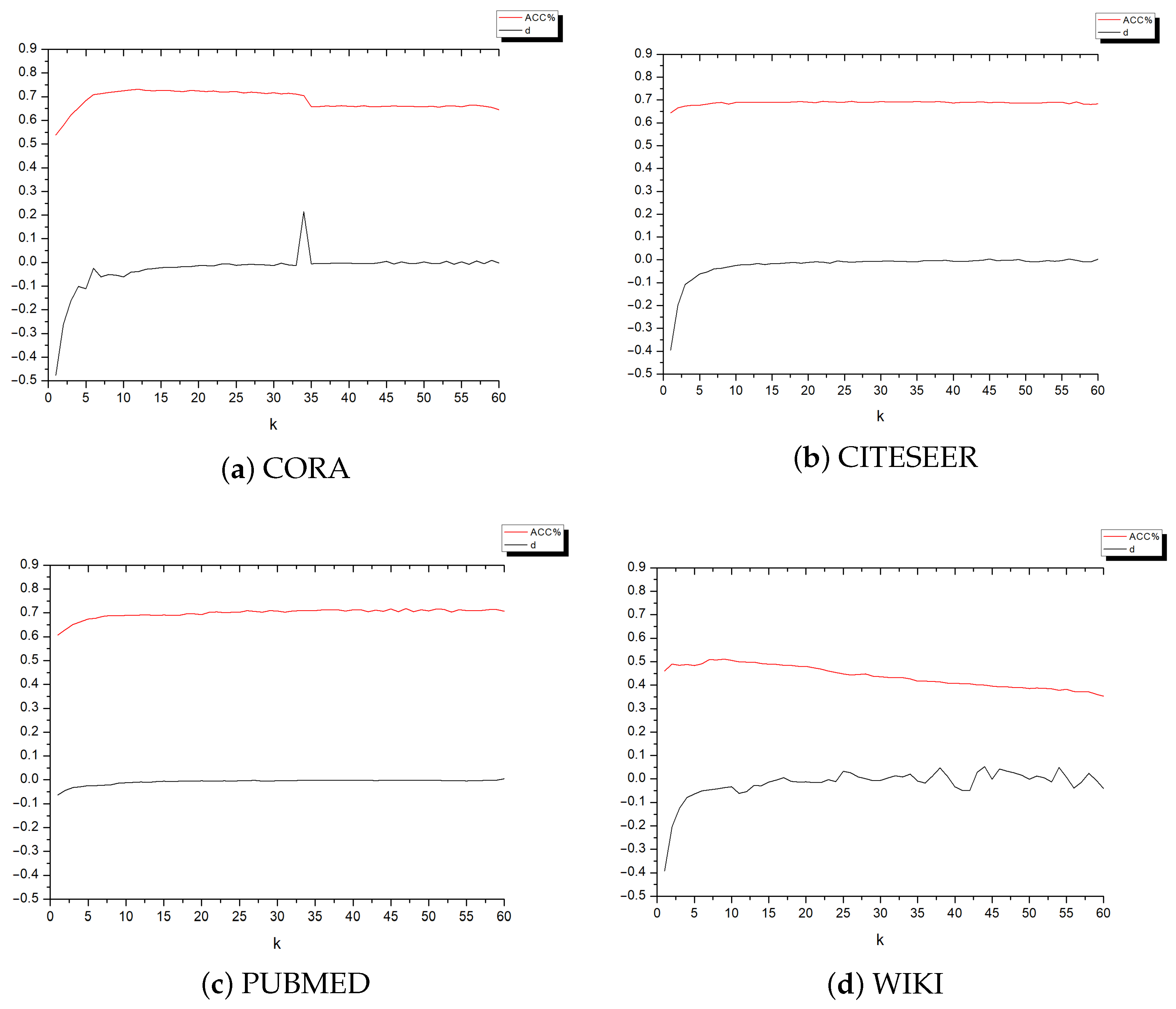
When it comes to the experiment that evaluates the cost of choosing the optimal k-value, the methods of the two different strategies (3WDAGC and AGC) each yielded the same value of k. However, unlike AGC, which obtains the value of k with a violent enumeration method, the number of steps for 3WDAGC to obtain the optimal k-value to be used for the subsequent tasks is significantly reduced. This is easy to see from the comparative experiment results in Figure 3 and Table 3.
Obviously, the average number of steps to find a relatively suitable value of k has been drastically reduced due to the introduction of the three-way decision idea.
The following can be inferred: (1) The optimal k-order convolutional kernel is selected for different datasets, and 3WDAGC is more adaptive compared to the AGC (the average optimization-seeking step is reduced). (2) 3WDAGC solves the selection of the initial k without the need to specify a specific k-value.

5.5. In-Depth Analysis of 3WDAGC

To further understand the properties and strengths of our proposed method, we conducted a series of in-depth analyses, including parameter sensitivity, an ablation study on the search strategy, scalability tests, and qualitative case studies.

5.5.1. Parameter Sensitivity Analysis

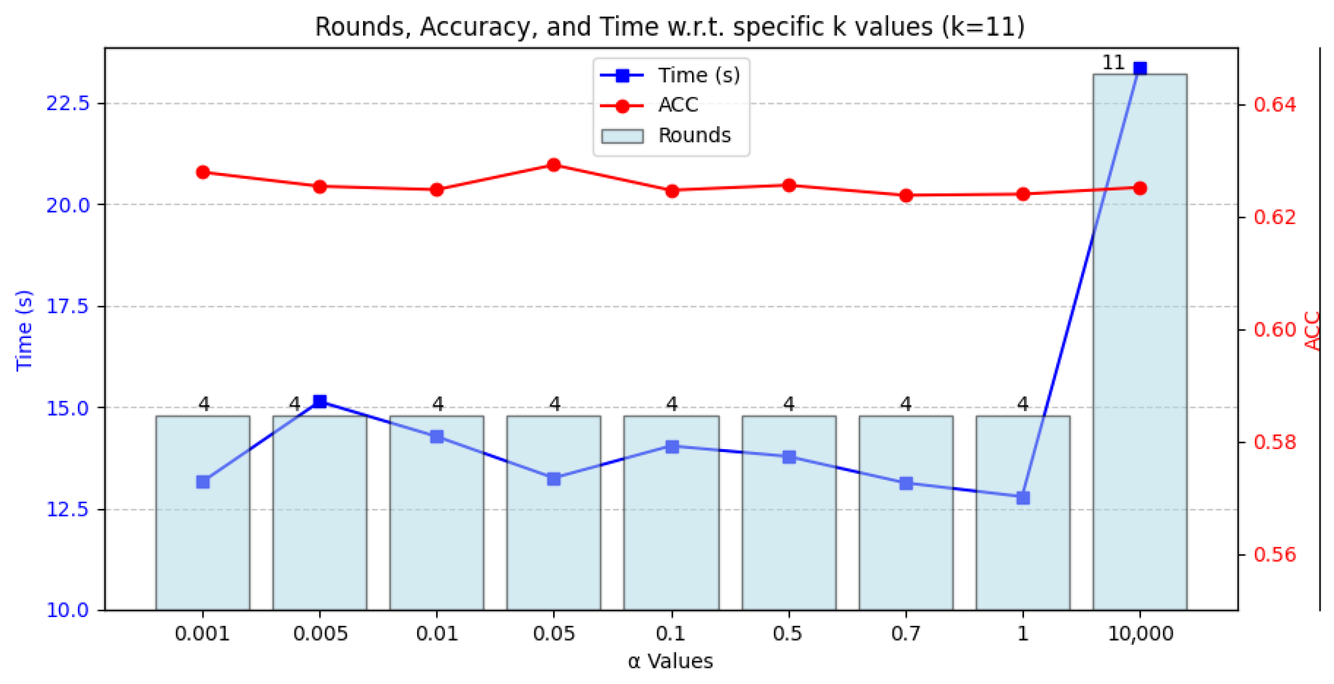
To evaluate the robustness of our framework, we analyze the sensitivity of the hyperparameter α , which functions as a key threshold in our three-way decision model. The experiment was conducted on the Cora dataset, where we varied α across a wide range of values to observe its effect on accuracy (ACC), computational time, and the number of rounds required for convergence. As illustrated in Figure 4, our model demonstrates considerable stability for α in the range of [0.001, 1]. Within this interval, the number of rounds remains constant at 4, while the accuracy and time exhibit only minor fluctuations. This indicates that our method is robust and not overly sensitive to the precise choice of α , which is a highly desirable property for practical applications as it reduces the need for extensive hyperparameter tuning. Further analyses on the Citeseer and Wiki datasets, provided in Appendix B, confirm this robust behavior across different graph structures.
Furthermore, the analysis confirms a theoretical aspect of our model: when α is set to a sufficiently large value (e.g., 10,000), the model is designed to converge to the standard AGC model. This behavior is empirically validated by the results, which show a sharp increase in the number of rounds to 11 and a corresponding surge in execution time, while the accuracy remains comparable. This confirms the model’s behavior as designed and highlights the efficiency of our approach within its typical operational range.

5.5.2. Ablation Study on the Search Strategy

To validate the effectiveness of our proposed three-way decision search strategy, we conducted an ablation study. We compared our full 3WDAGC model against a variant, named “3WDAGC-Linear,” which employs the same graph convolution and clustering pipeline but replaces the adaptive search with a simple fixed-step linear search ( k = k + 1 ). The results, summarized in Table 4, compellingly demonstrate the superiority of our adaptive approach. The 3WDAGC model not only achieves comparable or better clustering performance but does so with a significant reduction in search time, which confirms the efficiency of our search strategy.

5.5.3. Qualitative Analysis and Case Studies

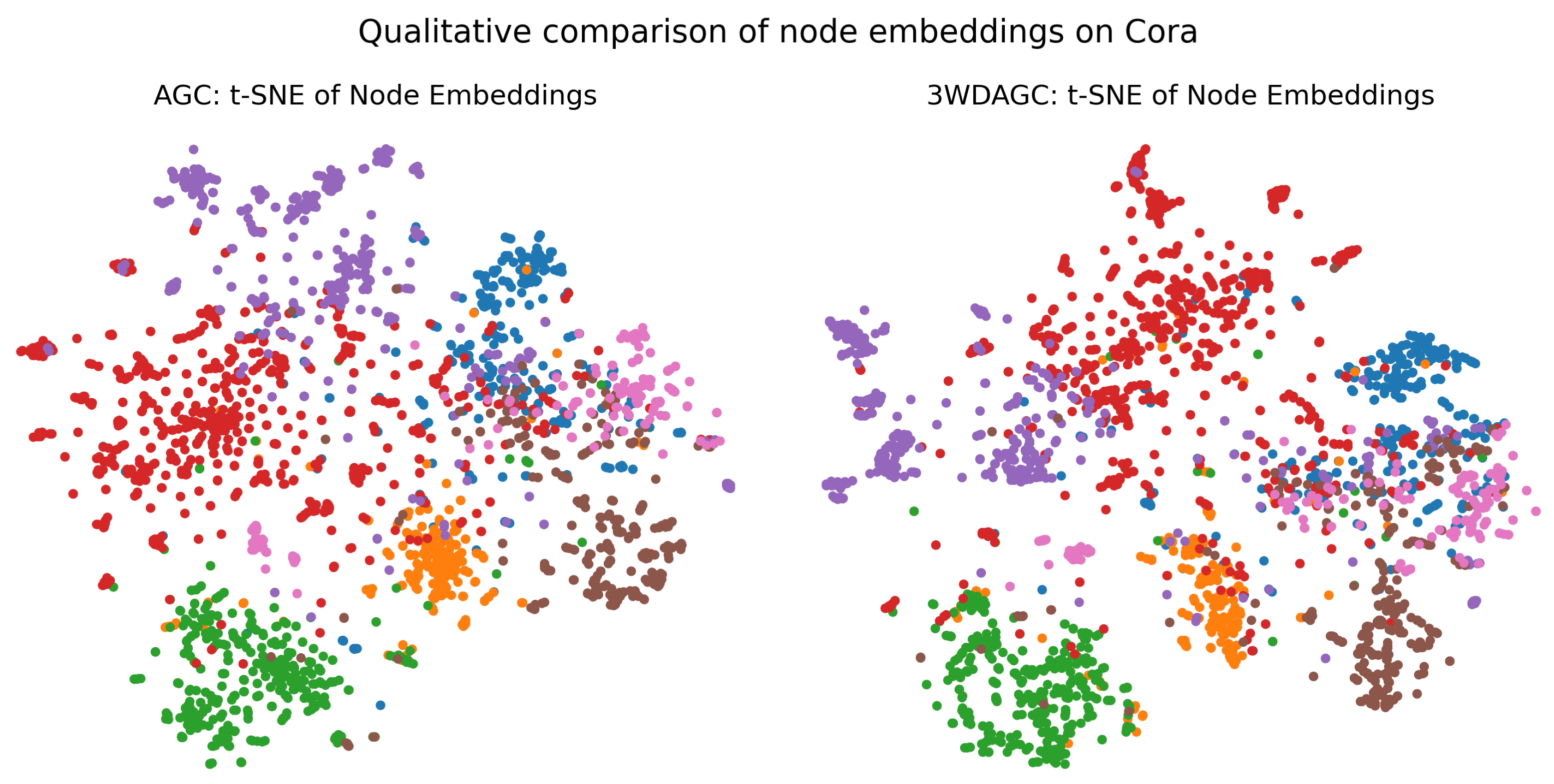
To provide a more intuitive understanding of our method’s behavior, we conducted a qualitative analysis. Figure 5 presents a side-by-side comparison of the t-SNE visualizations for the node embeddings generated using the optimal k found by the baseline AGC and our 3WDAGC on the Cora dataset. The visualization offers clear evidence of our method’s effectiveness. It is evident that the embedding space produced by 3WDAGC (right) exhibits more distinct and well-separated clusters, with clearer margins between different classes (e.g., the red and green clusters), compared to the embeddings from AGC (left). In the AGC plot, several clusters show significant overlap and less defined boundaries. This visual evidence corroborates our quantitative results, showing that our adaptive search strategy finds a convolution order that leads to a more effective and discriminative feature representation for clustering.

6. Conclusions

In this paper, we introduced 3WDAGC, a novel framework that successfully integrates three-way decision theory into adaptive graph convolution for deep clustering. Our method automatically finds a suitable convolution order k by efficiently navigating the trade-off between capturing global structure and preventing over-smoothing. The core contribution is an adaptive search algorithm that yields state-of-the-art clustering performance while significantly accelerating the hyperparameter tuning process compared to linear or brute-force searches. More broadly, our work serves as a proof of concept, demonstrating the potential of decision-theoretic principles to build more intelligent and automated graph representation learning models. This approach marks a step away from manual or exhaustive hyperparameter tuning towards more efficient and robust model self-configuration.
Despite these promising results, the current scope of our study naturally suggests several avenues for future research. The first challenge is scalability; the current implementation’s reliance on full-graph convolutions and the internal spectral clustering metric presents a bottleneck for massive graphs. Future work should therefore focus on integrating our adaptive search with scalable GNN strategies, such as graph sampling. A second consideration is generalizability. The search for an optimal k currently relies on an internal metric tied to spectral clustering, which could create a dependency. A key direction is to investigate lightweight, algorithm-agnostic metrics to ensure the learned embeddings are universally effective across different downstream algorithms. Finally, the scope of this work is focused on clustering for static, homogeneous graphs. Extending the adaptive framework to more complex structures (interaction networks in bioinformatics or transaction networks in finance), such as dynamic or heterogeneous graphs, and applying it to other tasks, like node classification and link prediction, are exciting avenues for future exploration [44,45,46].

Author Contributions

Conceptualization, W.L. and D.L.; Methodology, W.L.; Validation, K.C. and S.S.; Formal analysis, D.L. and C.W.; Investigation, W.L. and D.L.; Resources, W.L.; Data curation, W.L. and C.W.; Writing—original draft, W.L., C.W. and K.C.; Writing—review & editing, W.L. and D.L.; Supervision, W.L. and D.L.; Funding acquisition, D.L. All authors have read and agreed to the published version of the manuscript.

Funding

This research received no external funding.

Institutional Review Board Statement

Not applicable.

Informed Consent Statement

Not applicable.

Data Availability Statement

The data presented in this study are available on request from the corresponding author.

Conflicts of Interest

The authors declare no conflicts of interest.

Appendix A. Parameter Configuration

Table A1 details the hyperparameter settings used for the 3WDAGC framework in our experiments. These parameters were kept consistent across all datasets to ensure a fair and robust evaluation.
Table A1. Hyperparameter settings for 3WDAGC.
ParameterValueDescription
α 0.02The upper threshold in the three-way decision strategy, controlling the switch from accelerated to fine-grained search.
β 0The lower threshold, fixed at zero for all experiments.
Initial kRandomInt(1, 10)The initial convolution order k is randomly selected from the integer range [1, 10].
Initial b1The initial step size for the search algorithm.
Random Seed42A fixed random seed was used for all experiments to ensure reproducibility.

Appendix B. Additional Sensitivity Analysis

To further validate the robustness of our method, we conducted additional sensitivity analyses for the hyperparameter α on the Citeseer and Wiki datasets. The results, shown in Figure A1, are consistent with those on the Cora dataset. They demonstrate that 3WDAGC’s performance and search efficiency remain stable across a wide range of α values (e.g., [0.001, 1]), reinforcing that our method does not require extensive hyperparameter tuning.
Figure A1. Analysis of parameter sensitivity on Citeseer (left) and Wiki (right) datasets.
Applsci 15 09391 g0a1

References

  1. Kipf, T.N.; Welling, M. Semi-supervised classification with graph convolutional networks. In Proceedings of the 5th International Conference on Learning Representations, Toulon, France, 24–26 April 2017. [Google Scholar]
  2. Aljalbout, E.; Golkov, V.; Siddiqui, Y.; Strobel, M.; Cremers, D. Clustering with Deep Learning: Taxonomy and New Methods. arXiv 2018, arXiv:1801.07648. [Google Scholar] [CrossRef]
  3. Zhou, S.; Xu, H.; Zheng, Z.; Chen, J.; Zhao, L.; Bu, J.; Wu, J.; Wang, X.; Zhu, W.; Martin, E. A Comprehensive Survey on Deep Clustering: Taxonomy, Challenges, and Future Directions. arXiv 2022, arXiv:2206.06539. [Google Scholar] [CrossRef]
  4. Wang, C.; Pan, S.; Long, G.; Zhu, X.; Jiang, J. Mgae: Marginalized graph autoencoder for graph clustering. In Proceedings of the 2017 ACM on Conference on Information and Knowledge Management, Singapore, 6–10 November 2017; pp. 889–898. [Google Scholar]
  5. Zhang, X.; Liu, H.; Li, Q.; Wu, X.M.; Zhang, X. Adaptive graph convolution methods for attributed graph clustering. IEEE Trans. Knowl. Data Eng. 2023, 35, 12384–12399. [Google Scholar] [CrossRef]
  6. Min, E.; Guo, X.; Liu, Q.; Zhang, G.; Cui, J.; Long, J. A survey of clustering with deep learning: From the perspective of network architecture. IEEE Access 2018, 6, 39501–39514. [Google Scholar] [CrossRef]
  7. Nasraoui, O.; Ben N’Cir, C.E. An Introduction to Deep Clustering. In Clustering Methods for Big Data Analytics; Springer International Publishing: Cham, Switzerland, 2018; pp. 73–89. [Google Scholar]
  8. Liang, W.; Zhang, Y.; Xu, J.; Lin, D. Optimization of basic clustering for ensemble clustering: An information-theoretic perspective. IEEE Access 2019, 7, 179048–179062. [Google Scholar] [CrossRef]
  9. Newman, M.E.J. Finding community structure in networks using the eigenvectors of matrices. Phys. Rev. E 2006, 74, 036104. [Google Scholar] [CrossRef] [PubMed]
  10. Cao, S.; Lu, W.; Xu, Q. Grarep: Learning graph representations with global structural information. In Proceedings of the 24th ACM International on Conference on Information and Knowledge Management, Melbourne, Australia, 19–23 October 2015; pp. 891–900. [Google Scholar]
  11. Nikolentzos, G.; Meladianos, P.; Vazirgiannis, M. Matching node embeddings for graph similarity. In Proceedings of the 31st AAAI Conference on Artificial Intelligence, San Francisco, CA, USA, 4–9 February 2017; pp. 2429–2435. [Google Scholar]
  12. Perozzi, B.; Al-Rfou, R.; Skiena, S. Deepwalk: Online learning of social representations. In Proceedings of the 20th ACM SIGKDD International Conference on Knowledge Discovery and Data Mining, New York, NY, USA, 24–27 August 2014; pp. 701–710. [Google Scholar]
  13. Grover, A.; Leskovec, J. node2vec: Scalable feature learning for networks. In Proceedings of the 22nd ACM SIGKDD International Conference on Knowledge Discovery and Data Mining, San Francisco, CA, USA, 13–17 August 2016; pp. 855–864. [Google Scholar]
  14. Yang, C.; Liu, Z.; Zhao, D.; Sun, M.; Chang, E.Y. Network representation learning with rich text information. In Proceedings of the 24th International Joint Conference on Artificial Intelligence, Buenos Aires, Argentina, 25–31 July 2015; pp. 2111–2117. [Google Scholar]
  15. Wang, X.; Jin, D.; Cao, X.; Yang, L.; Zhang, W. Semantic community identification in large attribute networks. In Proceedings of the 2016 IEEE 16th International Conference on Data Mining (ICDM), Barcelona, Spain, 12–15 December 2016; pp. 265–271. [Google Scholar]
  16. Cao, S.; Lu, W.; Xu, G. Deep neural networks for learning graph representations. In Proceedings of the 30th AAAI Conference on Artificial Intelligence, Phoenix, AZ, USA, 12–17 February 2016; pp. 1145–1152. [Google Scholar]
  17. Ye, F.; Chen, C.; Zheng, Z. Deep autoencoder-like nonnegative matrix factorization for community detection. In Proceedings of the 27th ACM International Conference on Information and Knowledge Management, Turin, Italy, 22–26 October 2018; pp. 1393–1402. [Google Scholar]
  18. Chang, J.; Blei, D.M. Relational topic models for document networks. In Proceedings of the 12th International Conference on Artificial Intelligence and Statistics, Clearwater Beach, FL, USA, 16–18 April 2009; pp. 81–88. [Google Scholar]
  19. Bojchevski, A.; Günnemann, S. Bayesian robust attributed graph clustering: Joint learning of partial anomalies and group structure. In Proceedings of the 32nd AAAI Conference on Artificial Intelligence, New Orleans, LA, USA, 2–7 February 2018; pp. 2738–2745. [Google Scholar]
  20. Xia, R.; Pan, Y.; Du, L.; Yin, J. Robust multi-view spectral clustering via low-rank and sparse decomposition. In Proceedings of the 28th AAAI Conference on Artificial Intelligence, Québec City, QC, Canada, 27–31 July 2014; pp. 2149–2155. [Google Scholar]
  21. Wibisono, S.; Anwar, M.T.; Supriyanto, A.; Amin, I.H.A. Multivariate weather anomaly detection using dbscan clustering algorithm. J. Phys. Conf. Ser. 2021, 1869, 012077. [Google Scholar] [CrossRef]
  22. Liu, F.; Xue, S.; Wu, J.; Zhou, C.; Hu, W.; Paris, C.; Nepal, S.; Yang, J.; Yu, P.S. Deep learning for community detection: Progress, challenges and opportunities. In Proceedings of the 29th International Joint Conference on Artificial Intelligence, Yokohama, Japan, 7–15 January 2021; pp. 4981–4987. [Google Scholar]
  23. Tang, H.; Chen, K.; Jia, K. Unsupervised domain adaptation via structurally regularized deep clustering. In Proceedings of the IEEE/CVF Conference on Computer Vision and Pattern Recognition, Seattle, WA, USA, 13–19 June 2020; pp. 8722–8732. [Google Scholar]
  24. Meng, Y.; Zhang, Y.; Huang, J.; Zheng, Y.; Zhang, C.; Han, J. Hierarchical topic mining via joint spherical tree and text embedding. In Proceedings of the 26th ACM SIGKDD International Conference on Knowledge Discovery & Data Mining, Virtual Event, 6–10 July 2020; pp. 1908–1917. [Google Scholar]
  25. Yang, J.; Parikh, D.; Batra, D. Joint unsupervised learning of deep representations and image clusters. In Proceedings of the IEEE Conference on Computer Vision and Pattern Recognition, Las Vegas, NV, USA, 27–30 June 2016; pp. 5147–5156. [Google Scholar]
  26. Wang, X.; Shi, C.; Wang, Z.; Li, C.; Cheng, B. SIMPLE-GNN: A Simple and Efficient GNN for Large-scale Graph Learning. In Proceedings of the ACM Web Conference 2024 (WWW ’24), Singapore, 13–17 May 2024; pp. 2024–2035. [Google Scholar]
  27. Kipf, T.N.; Welling, M. Variational graph auto-encoders. arXiv 2016, arXiv:1611.07308. [Google Scholar] [CrossRef]
  28. Pan, S.; Hu, R.; Long, G.; Jiang, J.; Yao, L.; Zhang, C. Adversarially regularized graph autoencoder for graph embedding. In Proceedings of the 27th International Joint Conference on Artificial Intelligence, Stockholm, Sweden, 13–19 July 2018; pp. 2609–2615. [Google Scholar]
  29. Emadi, H.S.; Mazinani, S.M. A novel anomaly detection algorithm using dbscan and svm in wireless sensor networks. Wirel. Pers. Commun. 2018, 98, 2025–2035. [Google Scholar] [CrossRef]
  30. Su, X.; Xue, S.; Liu, F.; Wu, J.; Yang, J.; Zhou, C.; Hu, W.; Paris, C.; Nepal, S.; Jin, D.; et al. A comprehensive survey on community detection with deep learning. IEEE Trans. Neural Netw. Learn. Syst. 2022, 33, 3333–3353. [Google Scholar] [CrossRef] [PubMed]
  31. Hou, Z.; Liu, Y.; Wang, X.; Wei, Y.; Wang, P.; Dong, Y.; Tang, J. GraphMAE2: A Decoding-Enhanced Masked Autoencoder for Self-Supervised Graph Learners. In Proceedings of the 41st International Conference on Machine Learning (ICML), Vienna, Austria, 21–27 July 2024; pp. 19253–19275. [Google Scholar]
  32. Zhou, Q.; Zhou, W.; Wang, S. Cluster adaptation networks for unsupervised domain adaptation. Image Vis. Comput. 2021, 108, 104137. [Google Scholar] [CrossRef]
  33. Cai, X.; Huang, X.; Liang, H.; Wang, X. LightGCL: Simple and Effective Graph Contrastive Learning for Recommendation. In Proceedings of the 30th ACM SIGKDD Conference on Knowledge Discovery and Data Mining (KDD), Barcelona, Spain, 25–29 August 2024; pp. 187–197. [Google Scholar]
  34. Tixier, A.J.; Nikolentzos, G.; Meladianos, P.; Vazirgiannis, M. Graph classification with 2d convolutional neural networks. arXiv 2019, arXiv:1904.06132. [Google Scholar] [CrossRef]
  35. Lin, Z.; Kang, Z. Graph filter-based multi-view attributed graph clustering. In Proceedings of the 30th International Joint Conference on Artificial Intelligence, Montreal, QC, Canada, 21–26 August 2021; pp. 2723–2729. [Google Scholar]
  36. Li, H.J.; Wang, Z.; Cao, J.; Pei, J.; Shi, Y. Optimal estimation of low-rank factors via feature level data fusion of multiplex signal systems. IEEE Trans. Knowl. Data Eng. 2022, 34, 2860–2871. [Google Scholar] [CrossRef]
  37. Bo, D.; Wang, X.; Shi, C.; Zhu, M.; Lu, E.; Cui, P. Structural deep clustering network. In Proceedings of the Web Conference 2020, Taipei, Taiwan, 20–24 April 2020; pp. 1400–1410. [Google Scholar]
  38. Wang, M.; Liang, D.; Li, D. A two-stage method for improving the decision quality of consensus-driven three-way group decision-making. IEEE Trans. Syst. Man Cybern. Syst. 2023, 53, 2770–2780. [Google Scholar] [CrossRef]
  39. Zhu, J.; Ma, X.; Martinez, L.; Zhan, J. A probabilistic linguistic three-way decision method with regret theory via fuzzy c-means clustering algorithm. IEEE Trans. Fuzzy Syst. 2023, 31, 2821–2835. [Google Scholar] [CrossRef]
  40. Guo, L.; Zhan, J.; Zhang, C.; Xu, Z. A large-scale group decision-making method fusing three-way clustering and regret theory under fuzzy preference relations. IEEE Trans. Fuzzy Syst. 2023, 31, 4846–4860. [Google Scholar] [CrossRef]
  41. Li, Q.; Wu, X.M.; Liu, H.; Zhang, X.; Guan, Z. Label efficient semi-supervised learning via graph filtering. In Proceedings of the IEEE/CVF Conference on Computer Vision and Pattern Recognition, Long Beach, CA, USA, 15–20 June 2019; pp. 9574–9583. [Google Scholar]
  42. Van Der Maaten, L.; Hinton, G. Visualizing data using t-sne. J. Mach. Learn. Res. 2008, 9, 2579–2605. [Google Scholar]
  43. Fettal, C.; Labiod, L.; Nadif, M. Efficient graph convolution for joint node representation learning and clustering. In Proceedings of the 2022 International Joint Conference on Neural Networks (IJCNN), Padua, Italy, 18–23 July 2022; pp. 1–8. [Google Scholar]
  44. Fu, Y.; Yuan, J.; Song, G.; Wang, X.; Pan, S. Towards a Deeper Understanding of the Hub-induced Dilemma in Graph Neural Networks. In Proceedings of the Twelfth International Conference on Learning Representations (ICLR), Vienna, Austria, 7–11 May 2024. [Google Scholar]
  45. Behrouz, A.; Al-Tahan, M. Graph Mamba: Towards Learning on Graphs with State Space Models. In Proceedings of the Thirteenth International Conference on Learning Representations (ICLR), Vienna, Austria, 5–9 May 2025. [Google Scholar]
  46. Feng, Y.; Chen, K.; Zhang, Y.; Guo, J.; Tang, S.; Wang, Y.; Hooi, B. Large Language Models are Not Yet Effective Abstract Reasoners on Graphs. In Proceedings of the 2024 Conference on Empirical Methods in Natural Language Processing (EMNLP), Miami, FL, USA, 12–16 November 2024; pp. 15888–15902. [Google Scholar]
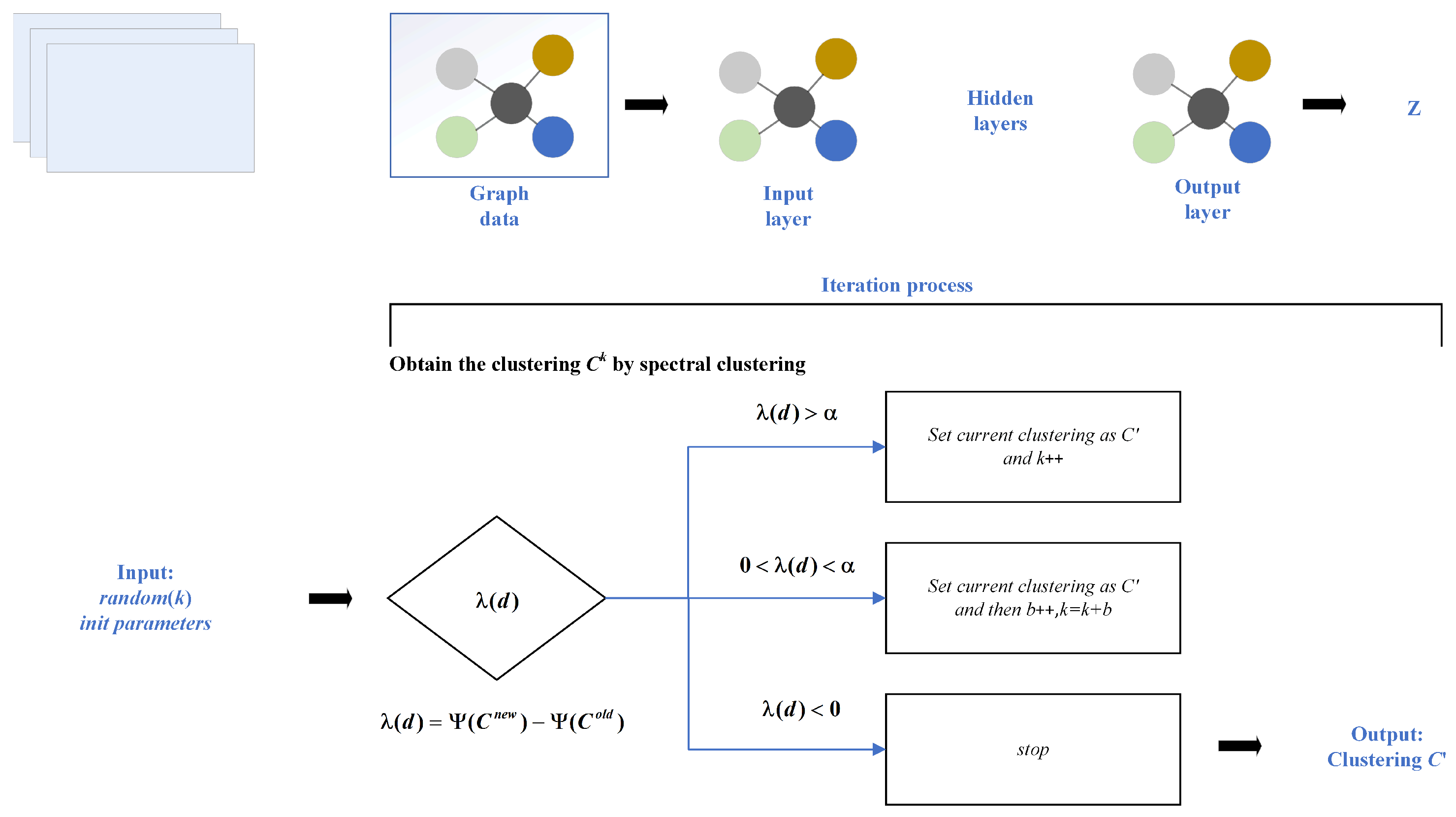
Figure 1. The overall pipeline of the proposed 3WDAGC framework.
Applsci 15 09391 g001
Figure 2. t-SNE visualization of Cora node features with different convolution order k. The data exhibits clear cluster structures with k = 12 . However, with k = 99 , the features are over-smoothed.
Applsci 15 09391 g002
Figure 3. The clustering performance (ACC) of 3WDAGC with respect to k on different datasets.
Applsci 15 09391 g003
Figure 4. Analysis of parameter sensitivity: clustering performance (ACC) and search steps on the Cora dataset with respect to the threshold α .
Applsci 15 09391 g004
Figure 5. Qualitative comparison of t-SNE visualizations for the optimal k found by AGC (left) and 3WDAGC (right) on the Cora dataset.
Applsci 15 09391 g005
Table 1. Dataset descriptions.
DatasetNodesEdgesFeaturesClasses
CORA2708542914337
CITESEER3327473237036
PUBMED19,71744,3385003
WIKI240517,981497317
Table 2. Clustering performance on datasets (%). Results are shown as mean ± standard deviation over 20 runs. The best results are in bold, and the second best are underlined.
MethodCORACITESEER
Acc NMI FM Acc NMI FM
k-means34.6516.7325.4238.4917.0230.47
Spectral-f36.2615.0925.6446.2321.1933.70
DeepWalk46.7431.7538.0636.159.6626.70
DNGR49.2437.2937.2932.5918.0244.19
GAE57.3140.6941.9741.2618.3429.13
VGAE61.3238.4541.5044.3822.7131.88
MGAE63.4345.5738.0163.5639.7539.49
ARGE66.6444.9061.9057.3035.0054.60
ARVGE62.3845.0062.7054.4026.1052.90
SDCN65.4547.1057.3265.7438.5162.07
GCC62.7149.8953.8967.3643.1565.46
AGC (k-means)66.43 ± 0.5152.79 ± 0.4865.41 ± 0.5554.41 ± 0.8832.23 ± 0.9152.04 ± 0.82
AGC (spectral)68.92 ± 0.4353.68 ± 0.4165.61 ± 0.4967.00 ± 0.4541.13 ± 0.5262.48 ± 0.48
3WDAGC (k-means)67.81 ± 0.4854.15 ± 0.4064.93 ± 0.5166.20 ± 0.5142.71 ± 0.4559.13 ± 0.58
3WDAGC (spectral)69.01 ± 0.4154.27 ± 0.3965.87 ± 0.4567.20 ± 0.4241.17 ± 0.5062.53 ± 0.46
MethodPUBMEDWIKI
AccNMIFMAccNMIFM
k-means57.3229.1257.3533.3730.2024.51
Spectral-f59.9132.5558.6141.2843.9925.20
DeepWalk61.8616.7147.0638.4632.3825.74
DNGR45.3515.3817.9037.5835.8525.38
GAE64.0822.9749.2617.3311.9315.35
VGAE65.4825.0950.9528.6730.2820.49
MGAE43.888.1641.9850.1447.9739.20
ARGE59.1223.1758.4141.4039.5038.27
ARVGE58.2220.6223.0441.5540.0137.80
SDCN64.8229.2363.7841.4737.9235.17
GCC69.7230.8768.7654.4251.1544.57
AGC (k-means)68.71 ± 0.3430.12 ± 0.4168.06 ± 0.3947.84 ± 1.1243.64 ± 1.0339.86 ± 1.21
AGC (spectral)69.78 ± 0.2931.59 ± 0.3368.72 ± 0.3147.65 ± 1.0845.28 ± 1.1540.36 ± 1.17
3WDAGC (k-means)69.85 ± 0.2530.37 ± 0.3969.37 ± 0.2848.35 ± 1.0146.14 ± 0.9841.69 ± 1.05
3WDAGC (spectral)69.62 ± 0.2831.73 ± 0.3169.17 ± 0.2947.96 ± 1.0545.82 ± 1.1140.87 ± 1.14
Table 3. Time consumed searching for an optimal k (5 runs): total time spent and average number of steps per round.
MethodCORACITESEERPUBMEDWIKI
Time
(Total)
Step
(avg.)
Time
(total)
Step
(avg.)
Time
(Total)
Step
(avg.)
Time
(Total)
Step
(avg.)
AGC153.512547.816622.615106.38
3WDAGC47.14147.99.2153.76.457.23.2
Table 4. Ablation study comparing 3WDAGC with its linear search variant on the Cora dataset.
MethodACCNMIFMTime (s)
3WDAGC-Linear0.66130.52740.651369.3
3WDAGC (Ours)0.67070.54190.654227.4
Disclaimer/Publisher’s Note: The statements, opinions and data contained in all publications are solely those of the individual author(s) and contributor(s) and not of MDPI and/or the editor(s). MDPI and/or the editor(s) disclaim responsibility for any injury to people or property resulting from any ideas, methods, instructions or products referred to in the content.