Hybrid CNN-Fuzzy Approach for Automatic Identification of Ventricular Fibrillation and Tachycardia

Abstract

Ventricular arrhythmias such as ventricular fibrillation (VF) and ventricular tachycardia (VT) are among the leading causes of sudden cardiac death worldwide, making their timely and accurate detection a critical task in modern cardiology. This study presents an advanced framework for the automatic detection of critical cardiac arrhythmias—specifically ventricular fibrillation (VF) and ventricular tachycardia (VT)—by integrating deep learning techniques with neuro-fuzzy systems. Electrocardiogram (ECG) signals from the MIT-BIH and AHA databases were preprocessed through denoising, alignment, and segmentation. Convolutional neural networks (CNNs) were employed for deep feature extraction, and the resulting features were used as input for various fuzzy classifiers, including Fuzzy ARTMAP and the Adaptive Neuro-Fuzzy Inference System (ANFIS). Among these classifiers, ANFIS demonstrated the best overall performance. The combination of CNN-based feature extraction with ANFIS yielded the highest classification accuracy across multiple cardiac rhythm types. The classification performance metrics for each rhythm type were as follows: for Normal Sinus Rhythm, precision was 99.09%, sensitivity 98.70%, specificity 98.89%, and F1-score 98.89%. For VF, precision was 95.49%, sensitivity 96.69%, specificity 99.10%, and F1-score 96.09%. For VT, precision was 94.03%, sensitivity 94.26%, specificity 99.54%, and F1-score 94.14%. Finally, for Other Rhythms, precision was 97.74%, sensitivity 97.74%, specificity 99.40%, and F1-score 97.74%. These results demonstrate the strong generalization capability and precision of the proposed architecture, suggesting its potential applicability in real-time biomedical systems such as Automated External Defibrillators (AEDs), Implantable Cardioverter Defibrillators (ICDs), and advanced cardiac monitoring technologies.

1. Introduction

Cardiac arrhythmias are common in industrialized countries and represent a significant cause of mortality. Among these, VF can trigger sudden death even in its less severe forms. Therefore, rapid identification of any ventricular arrhythmia is essential to apply appropriate treatments and protect the patient’s life. Although the triggers of arrhythmias may vary, they all share an origin in disturbances of the heart’s cellular electrical activity. Forensic studies have consistently shown that, in the majority of sudden death cases without apparent structural abnormalities in the heart, the underlying cause corresponds to electrical disorders of the myocardium. This suggests that VF may lead to a swift and non-recoverable breakdown in the electrical conduction system of the heart, posing a serious threat to the patient’s life [1,2].

In clinical practice, the immediate intervention for VF typically includes the application of an electrical shock through an AED [3]. These devices are currently available in many public spaces, such as shopping centers, airports, and sports stadiums. The procedure consists of administering a high-energy shock through the chest with the purpose of recovering the normal heart rhythm. Several studies [4,5,6] have revealed an inverse relationship between the time elapsed from the onset of VF and the effectiveness of defibrillation: the longer the delay, the lower the probability of success. These findings highlight the importance of acting quickly and applying the shock as soon as possible to maximize the chances of rhythm recovery. Hence, rapid and accurate detection of VF is critical to trigger timely defibrillation interventions.

The identification of VF and VT episodes from ECG signals has been extensively investigated using various statistical techniques. However, traditional approaches often fall short when it comes to accurately capturing the complex patterns associated with ventricular arrhythmias. Consequently, machine learning techniques have gained prominence as effective tools to overcome these limitations in arrhythmia detection. In [7], the wavelet transform was applied to distinguish between three types of ECG episodes: Normal, VT, and VF. Another study [8] employed a Gaussian-kernel support vector machine (SVM) based on morphological features to identify ventricular abnormalities. Real-time detection of shockable rhythms (VF/VT) using fixed thresholds was proposed in [9]. Beyond these approaches, other works have explored a variety of machine learning strategies for the detection and classification of ventricular arrhythmias. For example, the C4.5 decision tree classifier was used in [10]; the k-nearest neighbors (k-NN) algorithm was used in [11]; and Bayesian methods were adopted in [12]. Additionally, ref. [13] combined decision trees with Independent Component Analysis (ICA). These data-driven approaches, leveraging the power of machine learning, enhance both the precision and interpretability of cardiac signal analysis. By facilitating the extraction of relevant features, they play a crucial role in the development of more robust systems for the diagnosis and management of ventricular arrhythmias.

Analyzing ECG signals using traditional algorithms remains a considerable challenge, mainly due to the non-stationary and highly dynamic nature of biomedical signals. As a result, these conventional methods often fail to effectively capture the inherent variability and intricate patterns present in such data. In this context, CNNs have shown great potential for automatically and deeply extracting features from time–frequency (TF) representations of ECG signals, enabling the identification of complex patterns that are not easily captured by classical techniques. Nevertheless, while CNNs offer rich representations, their internal mechanisms are often opaque, and they typically require large datasets to achieve robust generalization—an important limitation in biomedical scenarios where data availability may be constrained.

To address these challenges and improve classification accuracy, feature selection techniques have been incorporated to optimize the input space, reduce dimensionality, and prioritize variables with higher discriminative power. Feature selection is essential to enhance model performance, especially given the noisy and non-stationary characteristics of ECG signals.

In parallel, fuzzy logic systems and neuro-fuzzy models have been widely studied in the context of arrhythmia detection, due to their capacity to handle the uncertainty inherent in biomedical signals and to represent knowledge in an interpretable manner [14]. Recent studies have combined fuzzy logic with machine learning approaches, including fuzzy support vector machines (Fuzzy SVMs) [15], fuzzy k-NN classifiers [16], and adaptive models such as ANFIS [17], reinforcing their relevance in clinical environments characterized by ambiguity and variability.

Moreover, inference systems based on Mamdani and Takagi-Sugeno fuzzy models have proven effective in distinguishing abnormal cardiac rhythms, offering a flexible representation of expert knowledge and enabling more robust decision-making compared to strictly binary classification methods [18].

Proposed Work

This study proposes a novel hybrid framework for the automatic detection of critical ventricular arrhythmias—specifically VF and VT—from ECG signals. The approach integrates several key components: TF domain transformations to capture the non-stationary characteristics of ECG signals, CNNs for deep and automatic feature extraction, advanced feature selection techniques to reduce dimensionality and enhance discriminative power, and fuzzy logic-based classifiers that provide interpretable and adaptive decision-making by handling uncertainty inherent in biomedical signals.

Unlike traditional end-to-end CNN classifiers, our method employs CNNs solely as feature extractors on TF representations, followed by a feature refinement stage. This modular design improves classification accuracy while reducing computational complexity and increasing model interpretability.

The fuzzy inference systems incorporated in the final classification stage are particularly suitable for clinical applications, as they allow the model to adapt to physiological variability and ambiguous cases commonly present in real-world ECG data.

Overall, the proposed framework aims to offer a robust, accurate, and interpretable solution with significant potential for deployment in clinical environments and embedded medical devices, including AEDs and portable cardiac monitors, where reliable and rapid arrhythmia detection is crucial.

To fulfill the objectives of this work, the remainder of this paper is organized as follows. Section 2 provides an overview of the classification algorithms evaluated in this study, including CNN, ANFIS, and Fuzzy ARTMAP. Section 3 outlines the materials used and details the preprocessing and transformation steps applied to the ECG signals. Section 4 describes the training procedures and evaluation metrics employed for model assessment. The results of the proposed method are presented in Section 5, followed by a discussion in Section 6. Finally, Section 8 offers concluding remarks and outlines potential directions for future research.

2. Machine Learning Models for Classification

2.1. Deep Learning Algorithms

Deep learning refers to a class of neural network models characterized by multiple layers that enable hierarchical representation learning. Inspired by the structure and function of the human brain, these models are designed to solve complex learning tasks across various domains. In particular, deep learning has demonstrated outstanding performance in computer vision applications. The most commonly used architectures include multilayer perceptrons (MLPs), CNNs, and recurrent neural networks (RNNs) [19]. Other specialized architectures, such as fully convolutional networks (FCNs), have been effectively applied to tasks like semantic segmentation [20].

2.1.1. Fundamental Concepts of Convolutional Neural Networks

This section provides an overview of the widely adopted CNN architecture, along with a description of the specific model utilized in this work.

CNNs are composed of specialized layers designed to extract and process meaningful features from image data. The convolutional layer applies a set of filters (kernels) to the input image through the convolution operation, preserving spatial relationships among pixels and generating feature maps that capture learned visual patterns [19]. Following convolution, the pooling layer reduces the spatial dimensions of the feature maps, thereby decreasing the number of parameters and computational load, while also mitigating overfitting. Common pooling strategies include max pooling and average pooling [19].

A nonlinear activation function, typically the Rectified Linear Unit (ReLU), is applied after convolution to introduce nonlinearity into the model, enabling the network to learn complex representations [21]. Finally, fully connected layers (FCLs) aggregate the extracted features and perform the final classification task, often employing the Softmax function to produce a probability distribution over output classes [19].

2.1.2. Loss Function

The loss function evaluates the prediction error between the model’s outputs and the actual labels and serves as the key feedback signal during training [22]. For multi-class classification problems, the cross-entropy loss is generally preferred, while mean squared error (MSE) is widely adopted in regression tasks. Choosing the appropriate loss function is crucial, as it directly influences how the model learns and converges during training.

2.1.3. Hyperparameter Optimization

Neural network hyperparameters are predetermined settings established before the training phase, as they are not adjusted during the learning process itself. These parameters critically influence model performance, making their careful tuning vital for achieving optimal accuracy and computational efficiency. Key hyperparameters typically include the following:

• Network Depth: The total number of layers, such as convolutional, activation (e.g., ReLU), pooling, and fully connected layers [23].
• Kernel Size: The dimensions of convolutional filters, commonly set to values like $3\times 3$, $5\times 5$, or $7\times 7$ [24].
• Filter Count: The number of filters applied in each convolutional layer, directly affecting the representational capacity of the extracted feature maps [25].
• Stride: The step size at which the convolutional filter moves over the input data; typical values are 1 or 2. Larger strides reduce the spatial resolution of outputs [26].
• Padding: Techniques such as ‘same’ or ‘valid’ padding control output spatial dimensions by adding pixels around the input [26].
• Activation Functions: Nonlinear transformations like ReLU, Leaky ReLU, or Sigmoid introduce nonlinearity; ReLU is favored for its efficiency and simplicity [27].
• Pooling Layers: Used to downsample feature maps, with max pooling and average pooling being the predominant choices, typically with window sizes of $2\times 2$ [28].
• Fully Connected Layers: Contain neurons whose number varies according to task complexity; the final layer’s size usually corresponds to the number of classification categories [29].
• Dropout Rate: A regularization parameter that randomly disables a fraction of neurons during training to reduce overfitting, commonly set between 0.2 and 0.5 [30].
• Batch Size: The number of training samples processed simultaneously in one iteration; smaller batches can improve convergence but increase computational cost [31].
• Number of Epochs: The number of complete passes the training algorithm makes over the entire dataset [32].
• Learning Rate: Controls the magnitude of weight updates during optimization; too small slows learning, while too large can cause divergence [33].
• Optimization Algorithm: Methods such as Stochastic Gradient Descent (SGD) [34], Adam, or RMSprop are used to iteratively adjust model parameters.

Optimal hyperparameter configurations depend heavily on dataset characteristics, task requirements, and computational constraints. Typically, practitioners rely on empirical experimentation and systematic search strategies to identify the best settings for their CNN models.

2.2. Fuzzy Logic-Based Models

This section presents fuzzy logic-based approaches applied to classification problems, highlighting the Fuzzy ARTMAP model. These methods combine fuzzy logic principles with machine learning techniques to handle uncertainty and facilitate learning [35].

2.2.1. Fuzzy ARTMAP

Fuzzy ARTMAP is a supervised neural network model based on Adaptive Resonance Theory (ART), designed for incremental classification and robust generalization in noisy environments. It combines fuzzy logic with stable learning mechanisms, incorporating techniques such as complement coding and dynamic match tracking.

Model Architecture

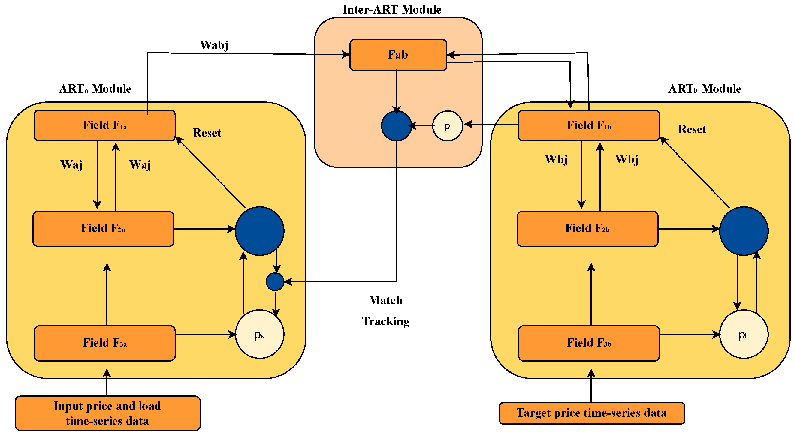
The model consists of two main modules: ARTa, which processes the input vector, and ARTb, which handles the target vector. Both are connected through an adaptive mapping field that links categories between the modules. Figure 1 illustrates the general architecture.

Main Components

• F0: Input layer where complement coding is applied to represent each value a along with its complement $1-a$, ensuring normalization and stability:

  $$I=(a,1-a),a\in {[0,1]}^n$$
• F1: Intermediate layer that compares the input vector with stored categories.
• F2: Category node layer representing class prototypes.
• WJ: Mapping field associating categories from ARTa with those in ARTb.

Training Process

• For each category j, a choice function measuring similarity between input I and prototype $w_j$ is calculated:

  $$T_j={\displaystyle \frac{\mathrm{similarity}(I,w_j)}{\mathrm{normalization}}}$$
• The winning category is selected as $J=arg{max}_j{T}_j$.
• The vigilance criterion is checked:

  $$\mathrm{match}={\displaystyle \frac{|I\wedge w_J|}{\left|I\right|}}\ge \rho$$
• If satisfied, weights are updated:

  $$w_J^{\mathrm{new}}=\beta (I\wedge w_J^{\mathrm{old}})+(1-\beta )w_J^{\mathrm{old}}$$
• If the category does not predict correctly, the vigilance parameter is adjusted dynamically:

  $$\rho \leftarrow \mathrm{match}+ϵ$$

Classification Phase

• Only ARTa is used to classify new inputs.
• ARTb is deactivated.
• Outputs are obtained from labels associated with the winning categories.

Key Parameters

• $\alpha$: controls sensitivity in category selection.
• $\beta$: regulates learning speed.
• $\rho$: defines the generalization level.
• $ϵ$: adjusts minimum precision in match tracking.

Trade-off

• Low $\rho$ leads to general categories (higher compression).
• High $\rho$ leads to specific categories (higher precision).
• Match tracking dynamically adjusts $\rho$ to improve performance when errors occur.

2.2.2. Membership Functions

Membership functions determine the degree of membership of a value x to a fuzzy set.

(a)

Triangular Function

$${\mu }_A\left(x\right)=\left\{\begin{array}{cc}0\hfill & x\le a\mathrm{or}x\ge c\hfill \\ {\displaystyle \frac{x-a}{b-a}}\hfill & a<x<b\hfill \\ {\displaystyle \frac{c-x}{c-b}}\hfill & b\le x<c\hfill \end{array}\right.$$

(b)

Trapezoidal Function

$${\mu }_A\left(x\right)=\left\{\begin{array}{cc}0\hfill & x\le a\mathrm{or}x\ge d\hfill \\ {\displaystyle \frac{x-a}{b-a}}\hfill & a<x<b\hfill \\ 1\hfill & b\le x\le c\hfill \\ {\displaystyle \frac{d-x}{d-c}}\hfill & c<x<d\hfill \end{array}\right.$$

(c)

Gaussian Function

$${\mu }_A\left(x\right)=exp\left(-{\displaystyle \frac{{(x-c)}^2}{2{\sigma }^2}}\right)$$

2.2.3. Fuzzy Inference System (FIS)

The Mamdani and Sugeno fuzzy models for a multi-input–single-output system can be represented as follows:

$$\mathrm{Mamdani}\mathrm{model}:R_i:\mathrm{IF}{x}_1\mathrm{is}{A}_{i1}\mathrm{AND}{x}_2\mathrm{is}{A}_{i2}\mathrm{AND}\dots \mathrm{THEN}y\mathrm{is}{B}_i$$

(1)

$$\mathrm{Sugeno}\mathrm{model}(\mathrm{zero}\mathrm{order}):R_i:\mathrm{IF}{x}_1\mathrm{is}{A}_{i1}\mathrm{AND}{x}_2\mathrm{is}{A}_{i2}\mathrm{THEN}y=c_i$$

(2)

where $A_{ij}$ and $B_i$ are fuzzy sets, and $c_i$ is a constant.

2.3. Neuro-Fuzzy Models

2.3.1. ANFIS

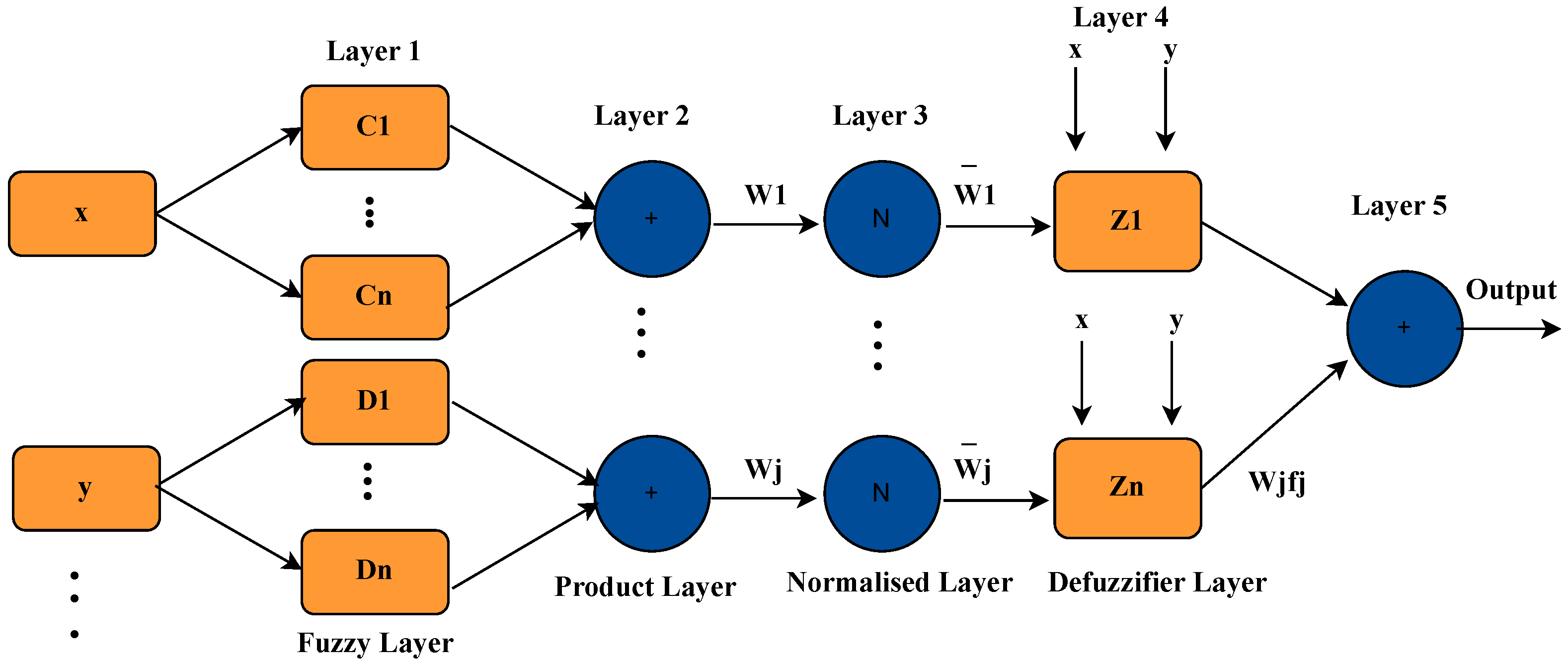
ANFIS (Adaptive Neuro-Fuzzy Inference System) integrates neural networks with fuzzy logic by employing a Takagi-Sugeno fuzzy inference system to model complex nonlinear relationships [17]. Its architecture consists of five layers (see Figure 2):

• Layer 1: Computes the fuzzy membership values of the inputs x and y using membership functions such as Gaussian curves:

  $$O_{1,i}={\mu }_{C_i}\left(x\right),O_{1,j}={\mu }_{D_j}\left(y\right)$$
• Layer 2: Calculates the firing strength of each fuzzy rule by multiplying the membership degrees:

  $$w_k={\mu }_{C_i}\left(x\right)·{\mu }_{D_j}\left(y\right)$$
• Layer 3: Normalizes the firing strengths to ensure they sum to one:

  $${\overline{w}}_i={\displaystyle \frac{w_i}{{\sum }_k{w}_k}}$$
• Layer 4: Produces weighted outputs using first-order Sugeno-type polynomial functions of the inputs:

  $${\overline{w}}_i{z}_i={\overline{w}}_i(p_{i}x+q_{i}y+r_i)$$
• Layer 5: Aggregates all the weighted outputs to produce the final output of the system:

  $$O_5=\sum _i{\overline{w}}_i{z}_i$$

Parameters such as the fuzzy sets $C_i$ and $D_j$, as well as the coefficients $p_i,q_i,r_i$, are learned during training to optimize model performance.

The fuzzy inference mechanism in ANFIS is governed by a set of if–then rules, which describe how the input variables relate to the output through linear functions. For a two-input, single-output system, a typical rule base is defined as follows [17]:

$$\begin{array}{cc}\hfill \mathrm{Rule}1:& \mathrm{IF}x\mathrm{is}{C}_1\mathrm{AND}y\mathrm{is}{D}_1;\mathrm{THEN}{z}_1=p_{1}x+q_{1}y+r_1\hfill \end{array}$$

(3)

$$\begin{array}{cc}\hfill \mathrm{Rule}2:& \mathrm{IF}x\mathrm{is}{C}_1\mathrm{AND}y\mathrm{is}{D}_2;\mathrm{THEN}{z}_2=p_{2}x+q_{2}y+r_2\hfill \end{array}$$

(4)

$$\begin{array}{cc}\hfill \mathrm{Rule}3:& \mathrm{IF}x\mathrm{is}{C}_2\mathrm{AND}y\mathrm{is}{D}_1;\mathrm{THEN}{z}_3=p_{3}x+q_{3}y+r_3\hfill \end{array}$$

(5)

$$\begin{array}{cc}\hfill \mathrm{Rule}4:& \mathrm{IF}x\mathrm{is}{C}_2\mathrm{AND}y\mathrm{is}{D}_2;\mathrm{THEN}{z}_4=p_{4}x+q_{4}y+r_4\hfill \end{array}$$

(6)

2.3.2. Classic Hybrid Training Method

ANFIS training adjusts two types of parameters:

• Premise parameters: $c_i,{\sigma }_i$, which define the membership functions.
• Consequent parameters: $p_i,q_i,r_i$, which represent linear output coefficients.

The training method combines the following:

• Estimation phase (Least squares): With premise parameters fixed, consequent parameters are estimated by solving the following equation:

  $$\widehat{\theta }={\left(A^{T}A\right)}^{-1}{A}^{T}Z$$

  where A is the regressor matrix, and Z is the desired output vector.
• Update phase (Gradient descent): With consequent parameters fixed, premise parameters are updated minimizing the mean squared error (MSE):

  $$E={\displaystyle \frac{1}{2}}\sum _{k=1}^M{(z_k-f_k)}^2$$
  The premise parameters $\theta$ are updated as follows:

  $${\theta }^{new}={\theta }^{old}-\eta {\displaystyle \frac{\partial E}{\partial \theta }}$$

  where $\eta$ is the learning rate.

This process is repeated until the error is sufficiently small or the maximum number of iterations is reached.

Table 1. Essential comparison between Fuzzy ARTMAP and ANFIS.

Feature	Fuzzy ARTMAP	ANFIS
Model type	Adaptive network based on competitive learning	Neuro-fuzzy system based on Takagi-Sugeno fuzzy inference
Learning	Supervised, incremental, and online	Supervised, batch training with backpropagation
Membership functions	Implicit, prototype-based	Explicit, Gaussian, triangular, etc.
Rule handling	Single winning rule per input	Multiple active rules with normalization

summarizes the key differences between the Fuzzy ARTMAP and ANFIS models.

3. Materials and Methods

This study proposes a hybrid methodology for the automatic detection of VF from ECG signals, combining deep learning for feature extraction with fuzzy logic-based classification. The general pipeline includes dataset preparation, signal preprocessing and segmentation, feature extraction using CNNs, feature selection to reduce dimensionality, and classification using fuzzy systems. Finally, the performance of the model is rigorously evaluated using standard classification metrics. Figure 3 illustrates the overall workflow.

3.1. Training and Testing Workflow

The complete pipeline was carefully divided into two independent stages: training and testing. This separation guarantees that no data leakage occurs between the two phases, ensuring that evaluation metrics reflect true model generalization.

• Training Phase:

  –

  ECG signals from the training set are first preprocessed: baseline wander and noise are removed, and signals are segmented into time windows (tws) using WRM.

  –

  Each windowed segment undergoes Hilbert Transform followed by the Pseudo Wigner–Ville (PWV) distribution to generate a high-resolution Time–Frequency Representation (TFR) matrix.

  –

  The TFR matrix is then converted into a fixed-size image (TFRI), suitable for CNN input.

  –

  These TFRIs are fed into a convolutional neural network, which performs automatic extraction of deep features. CNN training is carried out using only the training dataset, applying cross-validation to prevent overfitting.

  –

  The output features from the CNN are passed through several feature selection algorithms, such as Linear Discriminant Analysis (LDA), Mutual Information, Random Forest, Recursive Feature Elimination (RFE), Principal Component Analysis (PCA), and ANOVA (SelectKBest), to reduce dimensionality and retain the most informative parameters.

  –

  The reduced feature set is used to train fuzzy classifiers (Fuzzy ARTMAP and ANFIS), optimizing their internal parameters based on classification performance. This results in a fully trained hybrid model.

• Testing Phase:

  –

  ECG signals from the test set are processed following the same pipeline: preprocessing, segmentation, Hilbert Transform, and PWV-based TFR generation.

  –

  These new TFR matrices are also converted into TFRI images and passed through the already trained CNN. Importantly, the CNN is not retrained or modified in this phase.

  –

  The CNN extracts feature vectors from the TFRI images. These features are then reduced using the same feature selection scheme determined during the training phase.

  –

  Finally, the extracted features are input to the trained fuzzy classifier, which performs the final classification. Since the classifier model is already trained, no further learning occurs in this stage.

This two-phase setup ensures that the testing data remains entirely independent of the training process, providing a realistic assessment of the model’s ability to generalize to unseen data. All performance metrics reported in the Results section are derived exclusively from the testing phase.

3.2. Materials

The ECG recordings used in this study were obtained from the standard MIT-BIH Malignant VF database [36] and the AHA (2000 series) database [37]. To simulate realistic conditions for the use of an AED, no pre-selection of ECG episodes was performed prior to analysis. The dataset comprises 24 patient records, including the majority from MIT-BIH and a smaller subset from AHA. Each record contains approximately 30 min of continuous ECG signals with expert annotations.

The inclusion of AHA data aimed to increase the representation of ventricular tachycardia (VT) episodes and to balance the temporal distribution between VF and VT events. For this study, the ECG signals were categorized into four rhythm classes: Normal, VT, and VF, including flutter episodes, and Other Rhythms, comprising non-ventricular arrhythmias, noise, or artifacts.

3.3. Electrocardiographic Signal Preprocessing

Preprocessing of the ECG signal is a crucial step to ensure its quality prior to analysis or input into machine learning models. This stage primarily involves noise reduction and signal segmentation. To minimize common artifacts such as baseline wander (frequencies below 1 Hz), powerline interference (50/60 Hz), and electromyographic (EMG) noise, the signal was resampled at 125 Hz and processed with an 8th-order IIR bandpass Butterworth filter, with a passband between 1 Hz and 45 Hz [38,39]. This filtering preserves the relevant signal components while effectively removing unwanted noise.

After filtering, the signal was segmented by detecting Window Reference Marks (WRMs), which indicate the start of each tw. Following the approach in [40], a normal heart rate range of 50 to 120 beats per minute was assumed, defining minimum and maximum intervals between consecutive marks as $WR{M}_{min}=0.5$ s and $WR{M}_{max}=1.2$ s, respectively. Temporal windows of 1.2 s duration (150 samples) were then constructed starting from each $WR{M}_j$, as described in Equation (7).

$$\begin{array}{c}\hfill t{w}_j=[WR{M}_j,WR{M}_j+1.2\mathrm{s}];j=1,\dots ,N_{LMC}\end{array}$$

(7)

3.4. Conversion of the TFR Matrix into an Image for Classification

Once the TFR matrix is obtained for each time window (tw), combined with the Hilbert Transform (Ht), it is converted into a TFRI of fixed size $L_f\times L_t$, specifically $45\times 150$ pixels. This image is directly used as input to the CNN, allowing the model to process both temporal and spectral information simultaneously.

No additional feature extraction is applied to the TFRI, as it inherently encodes the essential characteristics of the ECG signal. The TFRI is generated using advanced time–frequency analysis techniques, notably the Wigner–Ville distribution, detailed in the following section.

3.5. Time–Frequency Representation

The Wigner–Ville Distribution (WV) is a widely used method for joint time–frequency analysis. In this work, it is applied directly to temporal windows of the ECG signal.

Alternatively, the analytic signal can be obtained via the Hilbert Transform before applying the WV distribution. This approach enhances the representation by focusing on the positive frequency spectrum of the signal.

Compared to the Pseudo Wigner–Ville (PWV) variant, the traditional WV distribution often generates interference and artifacts that complicate spectral interpretation [40]. For this reason, the PWV variant was ultimately chosen, which reduces these effects by applying a smoothing kernel $h\left(t\right)$.

Mathematically, the PWV is expressed by the following integral:

$$PW{V}_x(t,\nu )={\int }_{-\infty }^{+\infty }h\left(\tau \right)S\left(t+{\displaystyle \frac{\tau }{2}}\right)S^{*}\left(t-{\displaystyle \frac{\tau }{2}}\right)e^{-j2\pi \nu \tau }d\tau$$

(8)

where $S\left(t\right)$ represents the analyzed signal, $\tau$ is the time lag, t is the time instant, and h is the smoothing kernel in frequency. To reduce cross-term interference, the PWV employs the analytic signal rather than the original signal, effectively removing negative frequency components. The analytic signal $S\left(t\right)$, derived from the original signal $x\left(t\right)$, is defined in Equation (9):

$$S\left[x\right(t\left)\right]=x\left(t\right)+jH\left[x\right(t\left)\right]$$

(9)

where $H\left[x\right(t\left)\right]$ corresponds to the Htof $x\left(t\right)$, described in Equation (10):

$$H\left[x\left(t\right)\right]={\displaystyle \frac{1}{\pi }}\mathrm{P}.\mathrm{V}.{\int }_{-\infty }^{+\infty }{\displaystyle \frac{x\left(\tau \right)}{t-\tau }}d\tau$$

(10)

In the last equation, $\mathrm{P}.\mathrm{V}.$ indicates that the integral is taken in the sense of the Cauchy principal value.

In Figure 4, examples of time–frequency representations obtained using the PWV transform are presented for signals from the Normal, Other, VT, and VF classes. The intensity distributions reveal distinct patterns for each class. For Normal signals, the intensity is primarily concentrated in time, reflecting the presence of the QRS complex, and spans a wide frequency range. In contrast, signals corresponding to VF exhibit irregular intensity distributions along both the temporal and spectral axes, lacking a defined pattern.

4. Training and Evaluation of the Models

4.1. Training and Validation of CNN

CNN was progressively adjusted by incorporating and modifying layers while keeping hyperparameters constant during training.

The main objective was to identify layers that significantly improve performance in detecting VF. CNN was trained for 100 epochs using the Adam optimizer and categorical cross-entropy loss function.

To evaluate performance and prevent overfitting, cross-validation was applied with an 80% training and 20% testing split, repeated five times with different random partitions and results averaged. Metrics considered included sensitivity, specificity, accuracy, and F1 score.

The primary function of the CNN is to automatically extract relevant features from TFRI images, which are then used as input for fuzzy logic-based classifiers. The detailed architecture of the CNN, including kernel sizes, number of filters, and trainable parameters, is presented in

Table 2. Details of the proposed architecture for the CNN model.

Model	CNN
Layer	Kernel Size	Number of Filters	# of Parameters
Conv1	3 × 3	32	320
Max Pooling1	4 × 4	-	0
Conv2	3 × 3	64	18,496
Max Pooling2	4 × 4	-	0
FC1	128	-	991,360
FC2	256	-	33,024
Softmax	4	-	1028

.

4.2. Feature Extraction and Selection

The parameters extracted by the CNN from the TFRI images constitute the base dataset for training and evaluating the fuzzy classifiers. It is important to highlight that the split into training and testing sets was performed initially on the TFRI data, and this partition remained fixed throughout the entire process.

The parameters extracted from the signals in the training set are used to train the fuzzy logic models and to perform feature selection, without re-splitting or mixing the data. Similarly, the extracted parameters corresponding to the testing set—which were never seen by the CNN nor the selection process during training—are used solely for the final evaluation of the fuzzy classifiers, thus guaranteeing the independence of the test phase.

Various feature selection methods were applied, including both automatic and manual strategies, aiming to identify the most representative subset of parameters and reduce dimensionality without losing discriminative information.

4.3. Training and Evaluation of Fuzzy Logic-Based Classifiers

Training began with the Fuzzy ARTMAP algorithm, conducting multiple tests to compare its performance using different feature selection methods in order to determine the optimal classification configuration.

In parallel, for ANFIS only the set of parameters selected as optimal was used, evaluating different membership function configurations (triangular, Gaussian, among others) to optimize its performance.

For ANFIS, two approaches were implemented for the membership functions: an automatic one, where rules and functions are generated directly from the data, and a manual one, where specific membership functions were defined for output adjustment.

Performance evaluation was conducted using standard metrics such as accuracy, sensitivity, specificity, F1-score, and area under the ROC curve (AUC), allowing an exhaustive comparison of the different models and configurations.

Figure 5 shows the training loss and evaluation performance of the ANFIS model using a triangular membership function in the automatic configuration.

4.4. Performance Metrics for Classification

The performance of the different networks on the testing dataset was evaluated after training completion. The evaluation employed five key metrics: accuracy (acc), sensitivity (sens), specificity (spe), precision (pre), and F1-score [41,42].

5. Results

This section presents the results obtained from the two main classification approaches explored in this study: the Fuzzy ARTMAP classifier, evaluated under various feature selection strategies, and the ANFIS model, analyzed under both automatic and manual configurations. Model performance was assessed using confusion matrices, ROC curves, and standard evaluation metrics, including sens, spe, pre, F1-score, and overall acc. This comparative analysis highlights how feature selection and membership function design influence each classifier’s ability to generalize and discriminate among multiple classes

5.1. Manual ANFIS Analysis

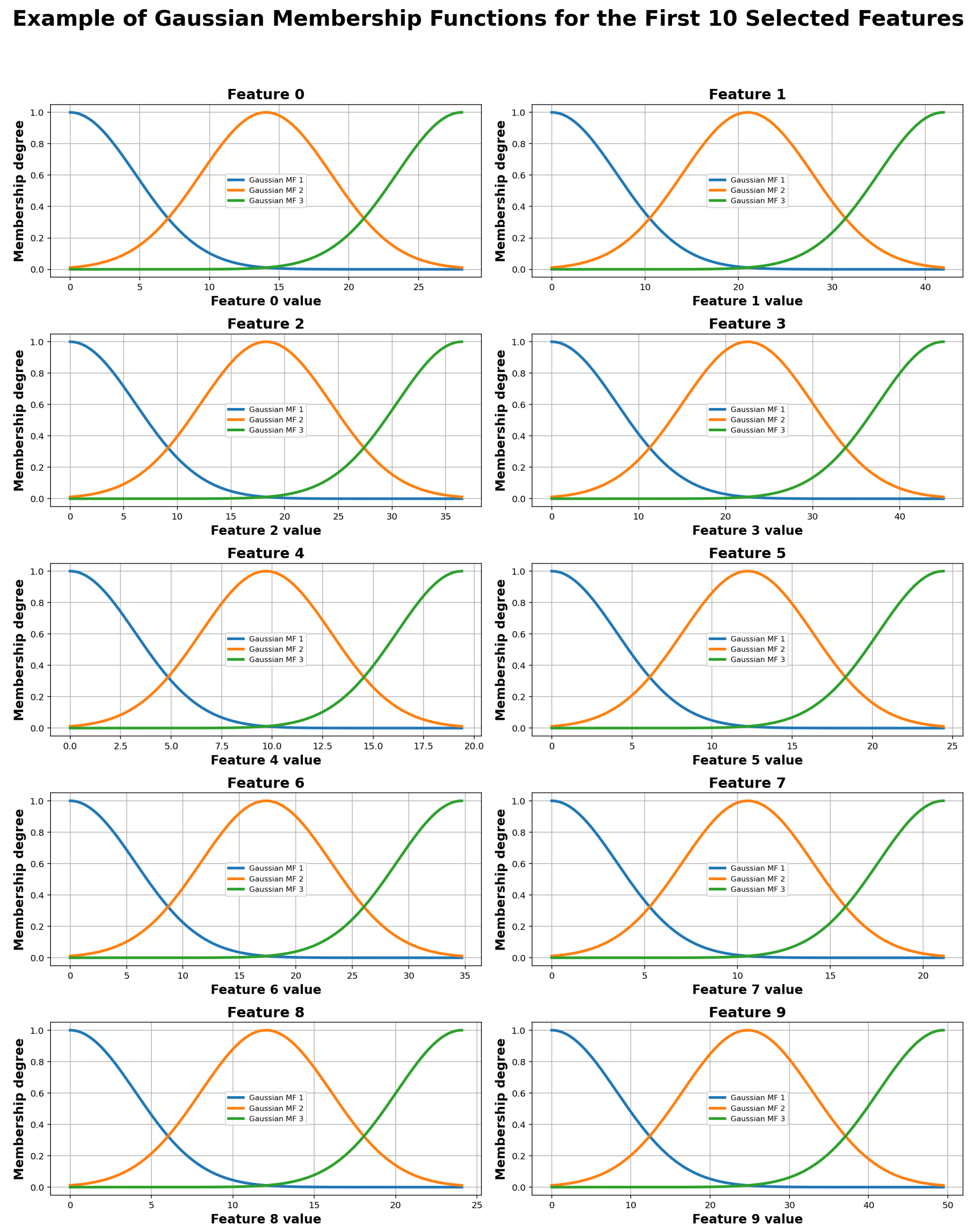
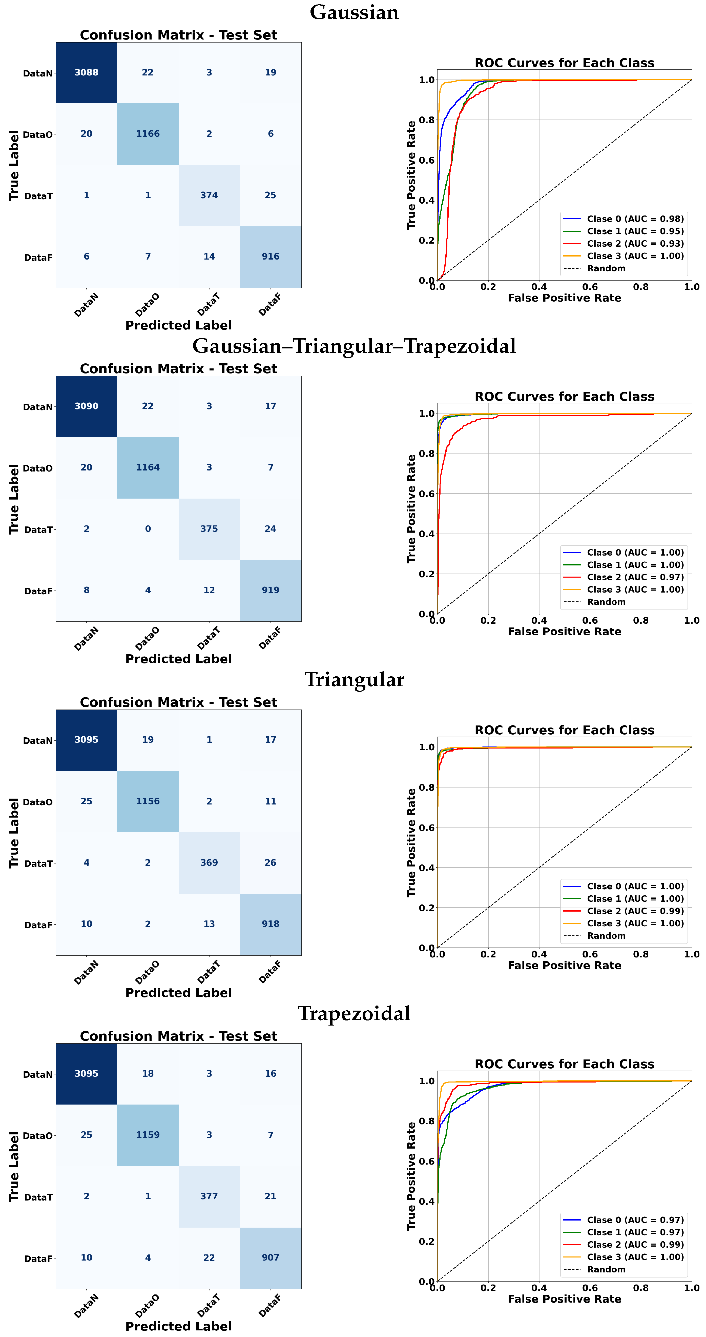
In the manual configuration, ten parameters were selected from the dataset to represent relevant signal characteristics. These parameters were assigned to membership functions of different types—Gaussian, triangular, and trapezoidal—whose shapes and positions were predefined based on expert knowledge.

Figure 6 illustrates examples of these membership functions for selected parameters, along with the classification performance metrics obtained for each class using this manual configuration. Unlike the automatic approach, this setup does not involve rule generation through training; instead, the inference relies on the manually defined membership functions and expert-defined decision rules.

This approach allows for direct control over the fuzzy partitions and can be useful when expert knowledge is available. However, it may lack the adaptability and efficiency of the automatic configuration when handling more complex or variable datasets.

5.2. Automatic ANFIS Analysis

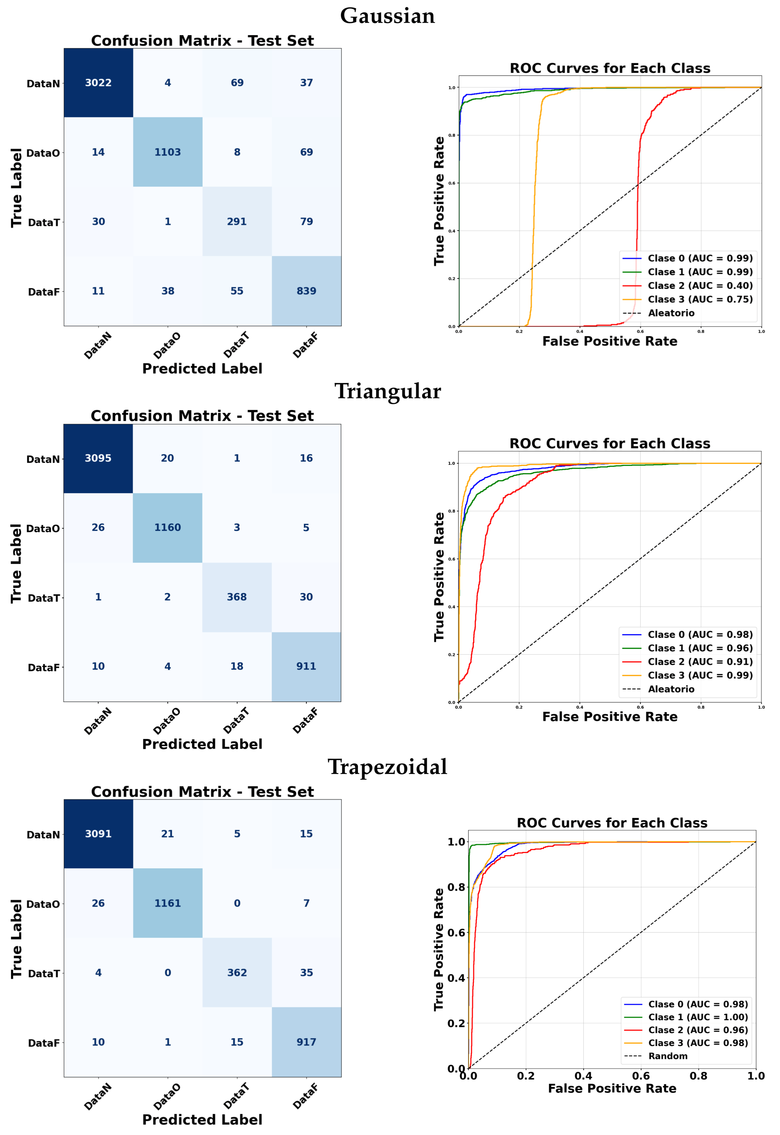
The ANFIS system was trained using 64 parameters previously selected from the CNN, which represent relevant and discriminative characteristics extracted from the ECG signals. These parameters were used as input for the adaptive fuzzy system with the goal of generating a reduced and efficient set of inference rules.

During the supervised training process, ANFIS generated a total of 10 fuzzy rules, which were constructed from the combination of multiple input parameters and their respective class labels (Normal, VF, VT, etc.). It is important to note that these rules are not individually assigned to each parameter; instead, each grouping of several attributes defines specific decision regions in the multidimensional feature space. Each rule represents a typical pattern associated with a class and defines a particular combination of input conditions that lead to a determined output. In this way, the system can capture complex relationships between physiological features without requiring a large number of rules, which favors interpretability and computational efficiency.

In this approach, training not only focuses on adjusting membership functions over the parameters but also centers on the generation and refinement of rules that encapsulate the knowledge learned from labeled data. This set of rules forms the basis for decision making in the ANFIS model and constitutes a key component of its generalization capability. An example of the trapezoidal membership functions generated for four selected parameters (0, 1, 6, and 7) is shown in Figure 7, where each parameter generates 10 membership functions.

5.3. Analysis of the ARTMAP Classifier

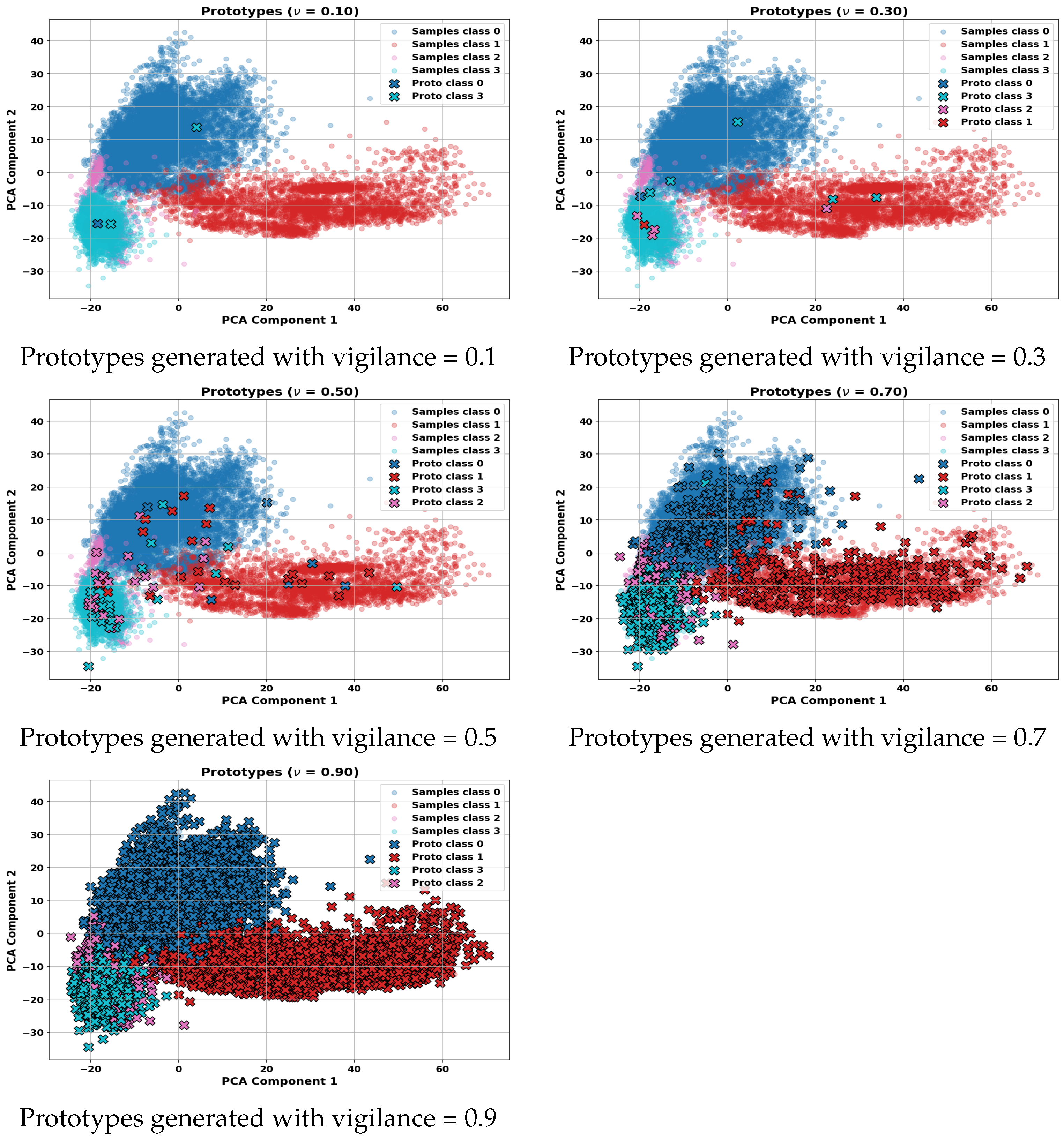
Figure 8 shows visual representations of the prototypes generated by the ARTMAP classifier at different levels of vigilance parameters, projected onto the plane of the first two principal components (PC1 and PC2). As the vigilance value increases, the number of prototypes generated also increases, reflecting greater specialization and segmentation of the feature space. This behavior allows for better class discrimination, but also increases model complexity and the risk of overfitting if not properly regulated.

Figure 9, Figure 10 and Figure 11 present a quantitative analysis of the effect of the vigilance parameter on the performance of the ARTMAP classifier.

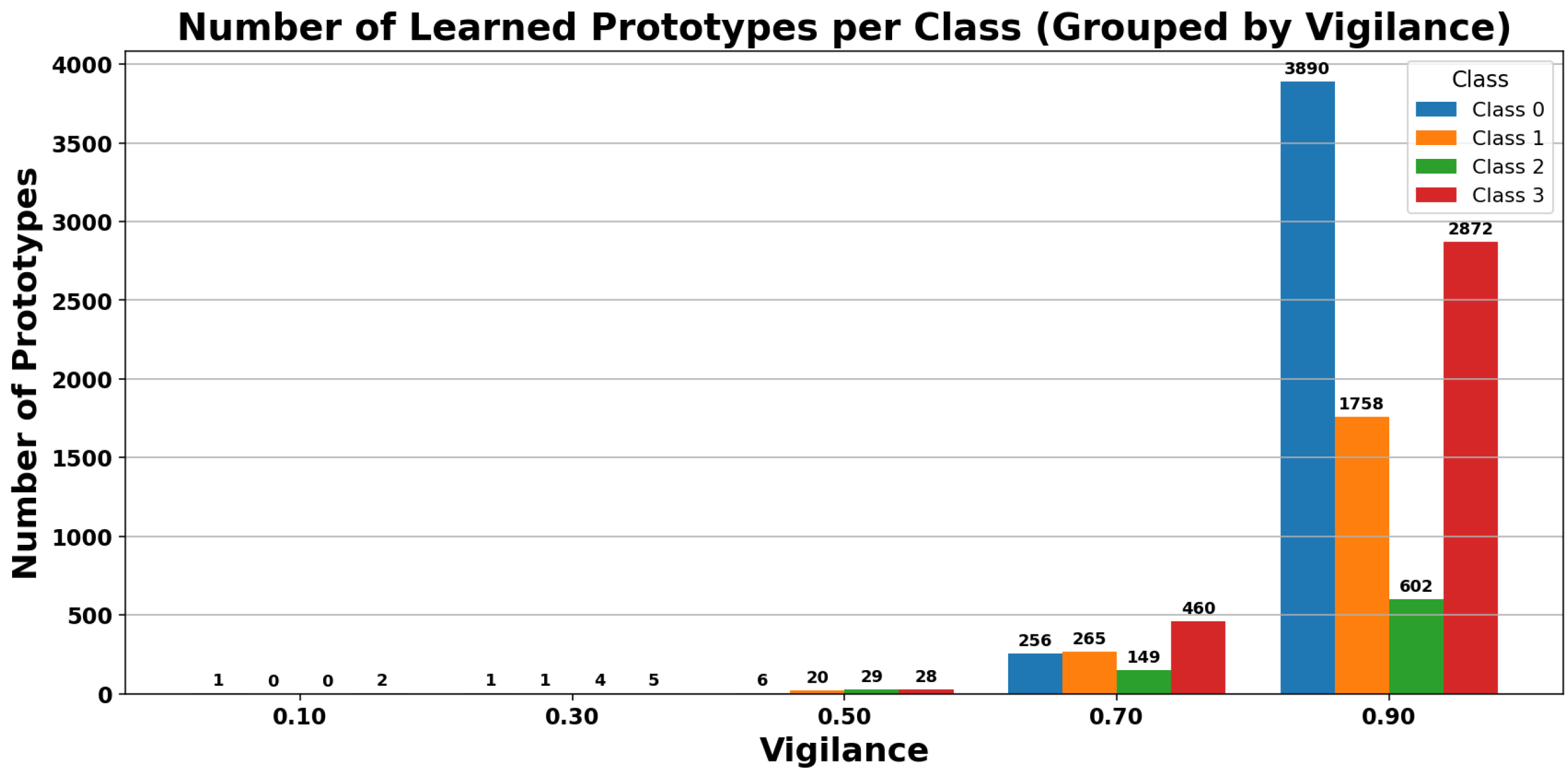
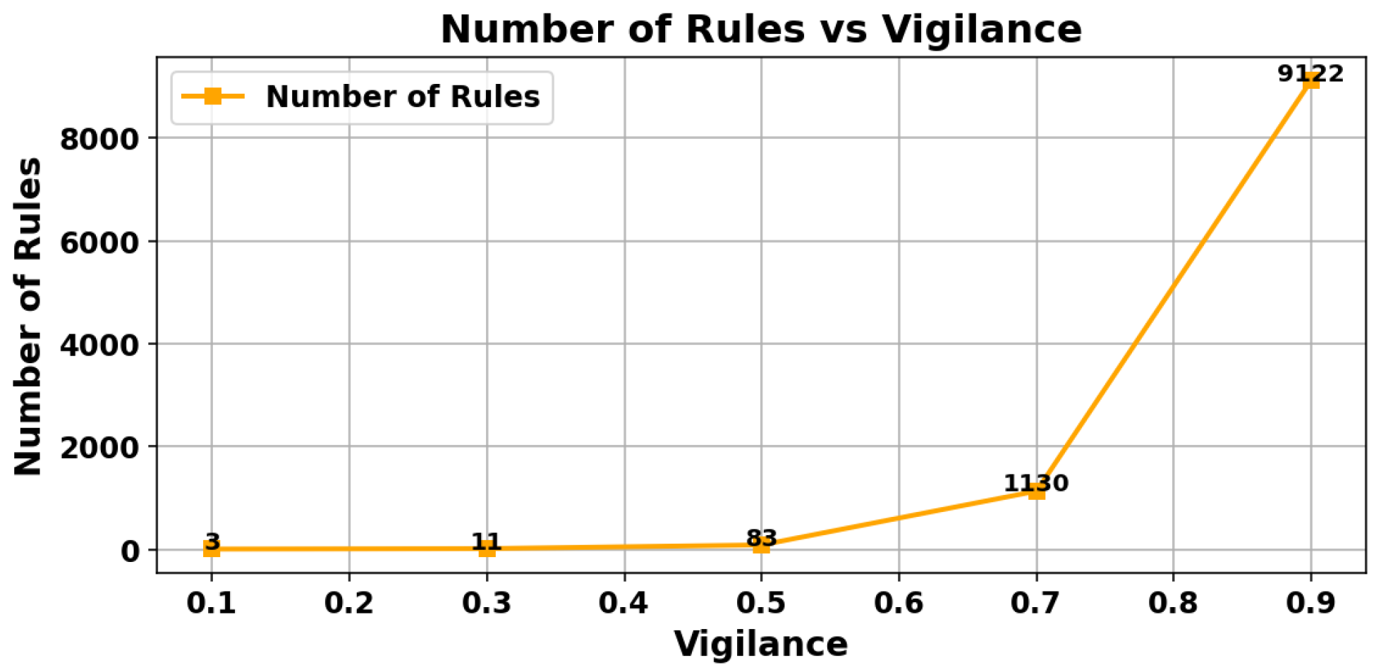
Figure 9 shows that the total number of prototypes increases as the vigilance parameter increases, confirming a greater segmentation of the feature space. Figure 10 presents the number of rules generated per class, allowing analysis of the complexity associated with each class and its contribution to the overall model behavior. Finally, Figure 11 illustrates the variation in classifier accuracy. Although initially an increase in vigilance improves performance, a saturation point is reached (around vigilance = 0.7), after which the accuracy stabilizes or even decreases, indicating potential overfitting of the model.

Selection of the Vigilance Parameter

In theory, the ART-B algorithm allows dynamic adjustment of the vigilance parameter through a mechanism known as match tracking. However, in this study, the standard ARTMAP version with manual vigilance tuning was employed, which enabled controlled analysis of the model’s behavior across different values of this parameter.

Vigilance values ranging from 0.1 to 0.9 were evaluated. The analysis focused solely on the accuracy metric, observing how it varied as a function of the parameter. Although values such as 0.7 offered an acceptable balance, the value of 0.9 achieved the highest classification accuracy. For this reason, vigilance = 0.9 was selected as the final configuration for the subsequent phases of this study, including its use in comparison with other classifiers such as ANFIS. This decision is based exclusively on performance criteria (accuracy), without considering complexity or the number of rules.

5.4. Execution Times and Classifier Performance

First, the performance of the FuzzyARTMAP classifier was evaluated using different feature selection methods, obtaining processing, selection, and prediction times for each case (see

Table 3. Processing, feature selection, and prediction times for FuzzyARTMAP classifier using different feature selection methods.

Selection Method	Processing Time (s)	CNN Parameter Extraction (s)	Selection TimE (s)	Prediction Time (s)	Total Time (s)
ANOVA	0.16–0.17	604.9	4.94 $\times {10}^{-7}$	0.30306	0.46306–0.47306
Mutual Information	0.16–0.17	604.9	0.000186	0.31375	0.47394–0.48394
Random Forest	0.16–0.17	604.9	3.56 $\times {10}^{-5}$	0.31008	0.47008–0.48008
RFE	0.16–0.17	604.9	96.93	0.00142	97.09142–97.10142
LDA	0.16–0.17	604.9	195.70	0.31612	196.17612–196.18612
PCA	0.16–0.17	604.9	294.41	0.63194	295.20194–295.21194

). Among all methods, Random Forest (RF) provided the best balance between accuracy and speed, with a total execution time of approximately 0.470–0.480 s, far below other methods such as RFE (∼97 s), LDA (∼196 s), or PCA (∼295 s), and relatively close to the times obtained by ANFIS. Due to this result, FuzzyARTMAP with RF was selected as a reference for comparative tests with ANFIS, as it offered high performance with low computational cost.

Subsequently, the execution time of the ANFIS classifier was analyzed, both in manual and automatic configurations, using different membership functions (triangular, Gaussian, trapezoidal, and combinations), as shown in

Table 4. Processing, feature selection, and prediction times for ANFIS (manual and automatic configurations).

Algorithm	Configuration	Processing Time (s)	CNN Parameter Extraction (s)	Feature Selection Time (ms)	Prediction Time (ms)	Total Time (s)
ANFIS Manual	Triangular	0.16–0.17	0.07–0.16	0.6049	0.9258	0.230–0.330
ANFIS Manual	Gaussian	0.16–0.17	0.07–0.16	0.6292	0.9596	0.231–0.331
ANFIS Manual	Trapezoidal	0.16–0.17	0.07–0.16	0.6076	0.9106	0.230–0.330
ANFIS Manual	Combination	0.16–0.17	0.07–0.16	0.6238	0.8998	0.231–0.331
ANFIS Automatic	Gaussian	0.16–0.17	0.07–0.16	0.6238	5.1	0.230–0.331
ANFIS Automatic	Triangular	0.16–0.17	0.07–0.16	0.6238	2.8	0.230–0.331
ANFIS Automatic	Trapezoidal	0.16–0.17	0.07–0.16	0.6238	4.9	0.230–0.331

. In all cases, ANFIS showed very low total execution times, ranging from 0.230 to 0.331 s, with a slight advantage for manual configurations in the prediction stage (≈0.9 ms versus 2.8–5.1 ms in automatic mode). Differences between membership types were minimal, showing that ANFIS, regardless of configuration, offers significantly faster execution than FuzzyARTMAP with heavier feature selection methods, and only slightly faster execution than FuzzyARTMAP with RF.

5.5. Confusion Matrices and ROC Curve Analysis

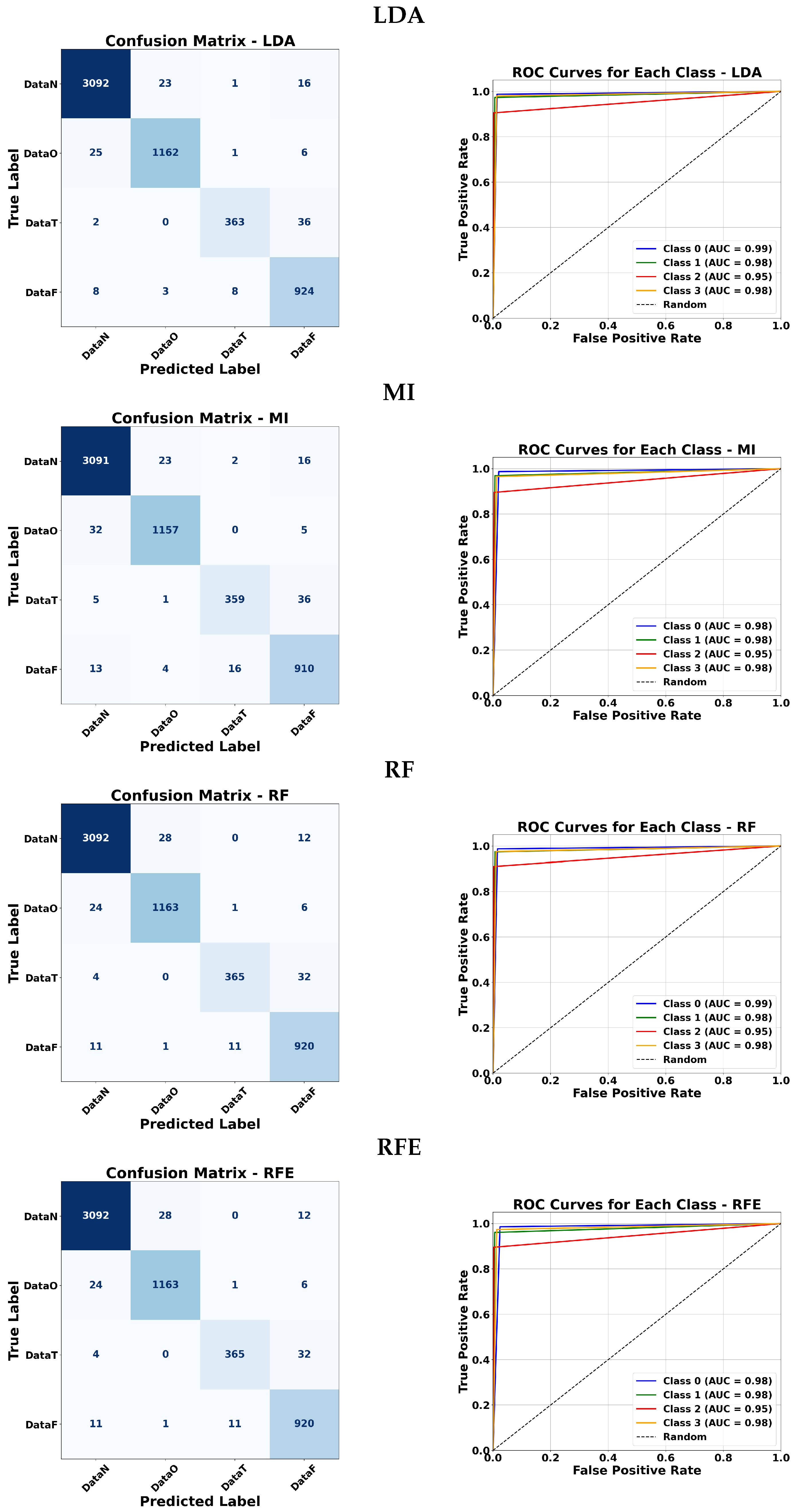
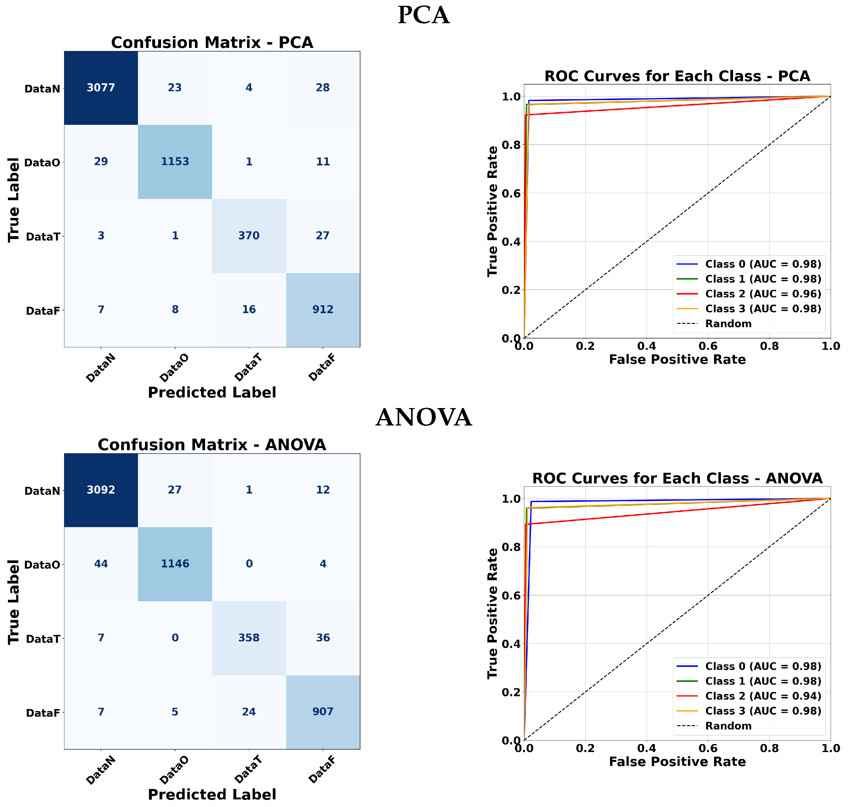
To further evaluate the effectiveness of each classifier, confusion matrices and ROC curves are presented. Figure 12, Figure 13, Figure 14 and Figure 15 illustrate the classification performance of ANFIS under various membership function configurations and of the Fuzzy ARTMAP model under different feature selection strategies. These visualizations allow a more detailed comparison in terms of sensitivity and specificity across the different approaches. In the confusion matrices, the background color indicates the magnitude of the values: darker triangles correspond to higher detection values, while lighter or white cells indicate lower values. Similarly, for the triangular membership functions, more intense colors represent higher values.

5.5.1. ANFIS Analysis

ANFIS classifiers were evaluated using four membership function types: Gaussian, triangular, trapezoidal, and a combination of the three. For the manual approach, Gaussian membership functions achieved very high AUC values for most classes, with slightly lower performance for class 3. Triangular and trapezoidal functions generally produced comparable results, with some cases reaching perfect AUC for classes 0, 1, and 3. The combination of all three membership functions maintained excellent performance across almost all classes.

For the automatic approach, Gaussian membership functions yielded a high AUC for classes 0 and 1, but a lower AUC for class 2. Triangular and trapezoidal functions generally improved the performance for class 2 while maintaining a high AUC for other classes. Overall, most membership functions achieved strong classification results, with minor variations between classes.

5.5.2. Fuzzy ARTMAP Analysis

Fuzzy ARTMAP classifiers were tested with various feature selection methods: LDA, MI, RF, RFE, PCA, and ANOVA. Across all methods, classes 0 and 1 consistently achieved very high AUC values (close to 0.98–0.99). Class 2 tended to have slightly lower values around 0.95–0.96, except for ANOVA which dropped slightly for class 1. Class 3 maintained high performance for all methods. Overall, LDA, MI, RF, and RFE produced nearly identical results, while PCA and ANOVA showed only minor variations. This indicates that the Fuzzy ARTMAP classifier is robust to different feature selection strategies and performs reliably across most classes.

5.6. Comparative Results: FuzzyARTMAPClassifier, ANFIS Manual, and ANFIS Automatic

The results presented in

Table 5. Comparative results for Normal: FuzzyARTMAPClassifier, ANFIS Manual, and ANFIS Automatic.

Method	Pre (%)	Sens (%)	Spe (%)	F1-Score (%)	Acc (%)
FuzzyARTMAP
LDA	0.00	0.00	100.00	0.00	44.76
Mutual Information	98.66	99.01	98.35	98.84	98.71
Random Forest	99.10	98.88	98.90	98.99	98.89
RFE	98.14	97.77	97.71	97.95	97.74
PCA	1.18	0.10	90.07	0.18	40.37
ANOVA	97.44	98.44	96.81	97.94	97.71
ANFIS Manual
Gaussian	99.13	98.60	98.94	98.86	98.01
Triangular	99.13	98.60	98.94	98.86	98.02
Trapezoidal	98.82	98.82	98.54	98.82	97.94
Gaussian + Triangular + Gaussian	99.04	98.66	98.82	98.85	98.01
ANFIS Automatic
Gaussian	99.09	98.70	98.89	98.89	98.78
Trapezoidal	98.81	98.62	98.55	98.71	97.95
Triangular	98.50	98.40	98.30	98.35	97.85

,

Table 6. Combined classification results—Other (FuzzyARTMAP and ANFIS).

Method	Pre (%)	Sens/Recall (%)	Spe (%)	F1-Score (%)	Acc (%)
FuzzyARTMAP
LDA	0.00	0.00	99.22	0.00	78.32
Mutual Information	98.14	97.32	99.51	97.73	99.05
Random Forest	98.07	97.91	99.49	97.99	99.15
RFE	95.59	96.31	98.82	95.95	98.29
PCA	21.72	78.31	24.73	34.01	36.01
ANOVA	96.07	94.05	98.97	95.05	97.94
ANFIS Manual
Gaussian	97.33	97.65	99.29	97.49	98.01
Triangular	97.41	97.65	99.31	97.53	98.02
Trapezoidal	98.05	97.07	99.49	97.56	97.94
Gaussian + Triangular + Gaussian	97.82	97.49	99.42	97.65	98.01
ANFIS Automatic
Gaussian	97.74	97.74	99.40	97.74	98.07
Trapezoidal	97.74	97.64	99.42	97.69	97.94
Triangular	97.50	97.40	99.30	97.45	97.85

,

Table 7. Classification results—VT (FuzzyARTMAP and ANFIS).

Method	Pre (%)	Sens/Recall (%)	Spe (%)	F1-Score (%)	Acc (%)
FuzzyARTMAPClassifier
LDA	6.57	92.27	0.08	12.26	6.60
Mutual Information	93.73	93.27	99.53	93.50	99.08
Random Forest	95.20	94.01	99.64	94.60	99.24
RFE	96.37	92.77	99.73	94.54	99.24
PCA	0.12	0.25	83.53	0.16	77.64
ANOVA	92.41	90.57	99.43	91.48	98.80
ANFIS Manual
Gaussian	94.92	93.27	99.62	94.09	98.01
Triangular	95.18	93.52	99.64	94.34	98.02
Trapezoidal	93.07	93.77	99.47	93.42	97.94
Gaussian + Triangular + Gaussian	95.42	93.52	99.66	94.46	98.01
ANFIS Automatic
Gaussian	94.03	94.26	99.54	94.14	99.18
Trapezoidal	92.44	93.77	99.16	93.10	97.93
Triangular	92.00	92.50	99.10	92.25	97.80

and

Table 8. Classification results—VF (FuzzyARTMAP and ANFIS).

Method	Pre (%)	Recall/Sens (%)	Spe (%)	F1-Score (%)	Acc (%)
FuzzyARTMAP
LDA	0.00	0.00	100.00	0.00	83.37
Mutual Information	95.87	95.97	99.17	95.92	98.64
Random Forest	95.72	97.14	99.13	96.42	98.80
RFE	95.21	97.03	99.03	96.11	98.69
PCA	0.41	0.11	94.90	0.17	79.14
ANOVA	95.23	95.33	99.05	95.28	98.43
ANFIS Manual
Gaussian	95.02	97.03	98.98	96.01	98.01
Triangular	95.02	97.14	98.98	96.07	98.02
Trapezoidal	95.27	96.18	99.05	95.72	97.94
Gaussian + Triangular + Gaussian	95.04	97.45	98.98	96.23	98.01
ANFIS Automatic
Gaussian	95.49	96.69	99.10	96.09	98.70
Trapezoidal	91.46	94.46	98.65	92.93	97.94
Triangular	91.00	94.00	98.50	92.00	97.80

highlight the main performance indicators—precision, sensitivity, specificity, F1-score, and overall accuracy—for each class and configuration. These tables allow a direct comparison between models and feature selection methods, showing which combinations achieve superior performance.

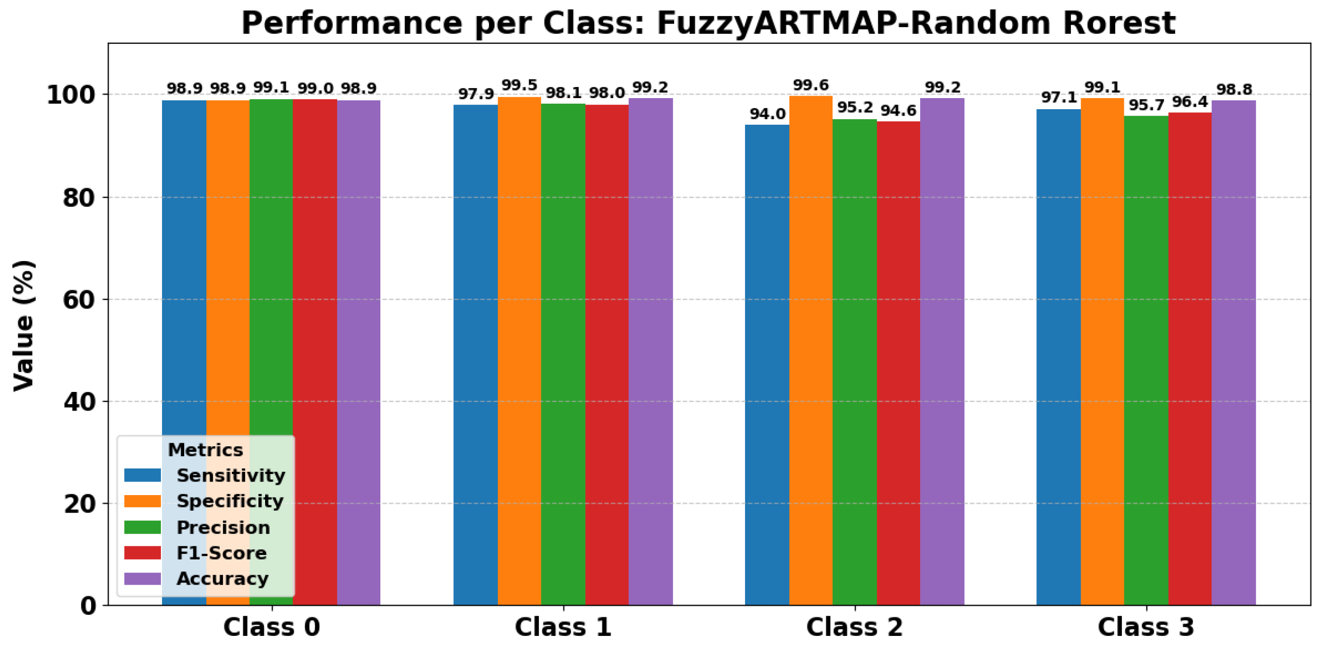
In particular, the FuzzyARTMAP model combined with Random Forest consistently achieves the highest performance across all four classes (Normal, Others, VT, and VF). Most metrics approach 99%, confirming that this combination outperforms other feature selection techniques such as LDA or PCA in terms of both accuracy and computational efficiency.

Figure 16 complements the tabular results by providing a visual overview of class-wise precision, sensitivity, specificity, F1-score, and accuracy. It clearly illustrates the robustness and consistently high-level performance of FuzzyARTMAP with Random Forest, reinforcing the numerical findings.

Overall, the combination of tabular data and graphical visualization provides a comprehensive understanding of model performance, demonstrating the superiority of FuzzyARTMAP with Random Forest over alternative configurations.

These results provide a strong baseline for comparing the performance of our FuzzyARTMAP configurations with other approaches reported in the literature. In the following section, we discuss how the achieved metrics—precision, sensitivity, specificity, F1-score, and overall accuracy—stand relative to other state-of-the-art methods, highlighting the improvements offered by the combination of FuzzyARTMAP with Random Forest.

As shown in

Table 9. Comparison of proposed CNN architecture for applications in detecting $Normal$, $Other$, $VT$, and $VF$ classes with other techniques.

Class	VF			VT			Other			Normal			Data Base
Techniques	Sens (%)	Spe (%)	Acc (%)	Sens (%)	Spe (%)	Acc (%)	Sens (%)	Spe (%)	Acc (%)	Sens (%)	Spe (%)	Acc (%)
This work, FuzzyARTMAP + RF	97.14	99.13	98.80	94.01	99.64	99.24	97.91	99.49	99.15	98.88	98.90	98.89	MITBIH, AHA
[43] Ht_TFR_CNN1 (Epochs = 50)	98.04	98.94	98.77	89.7	99.70	99	97.24	99.41	98.95	89.7	98.57	98.76	MITBIH, AHA
[43] Ht_TFR_CNN1 (Epochs = 100)	96.44	99.28	98.75	92.70	99.53	99.06	97.74	99.62	99.22	99.29	98.62	98.91	MITBIH, AHA
[43] Ht_TFR_CNN (Epochs = 100)	98.16	99.07	98.91	90.45	99.73	99.09	96.98	99.68	99.11	99.34	98.35	98.89	MITBIH, AHA
[43] InceptionV3 (Epochs = 6)	77.28	94.9	91.28	98.15	83.55	84.59	88.42	99.81	96.96	77.99	99.65	87.17	MITBIH, AHA
[43] AlexNet (Epochs = 6)	95.58	99.34	98.64	91.84	99.47	98.94	95.78	99.57	98.77	99.43	97.29	98.45	MITBIH, AHA
[43] MobilNet (Epochs = 6)	86.97	99.62	97.01	95.53	97.66	97.49	99.64	85.08	88.21	79.42	99.44	88.39	MITBIH, AHA
[43] VGGnet (Epochs = 6)	93.34	99.25	98.14	90.15	99.15	98.77	98.54	97.57	97.39	96.61	98.32	97.39	MITBIH, AHA
[40] SSVR, TFR	91	97		92.8	98.7		92.3	99.2		96.6	96.3		MITBIH, AHA
[40] ANNC and TFR	92.8	97		91.8	98.7		92.9	99		96.2	96.7		MITBIH, AHA
[40] BAGG, TFR	95.2	96.4		88.8	99.7		88.6	99.8		96.6	94.1		MITBIH, AHA
[40] I2-RLR and TFR	89.6	96.7		91	98.1		92.5	98.1		94.9	96.4		MITBIH, AHA
[44] PDI	84.34	96.77	94.26	82.25	98.53	97.38	92.86	97.15	96.19	93.09	92.14	92.65	MITBIH, AHA
[44] TDA	97.07	99.25	98.68	92.72	99.53	99.05	97.43	99.54	99.09	99.05	98.45	98.76	MITBIH, AHA

, the proposed FuzzyARTMAP classifiers, combined with Random Forest, were evaluated against several existing approaches to classify ventricular arrhythmias, including VT and VF. Importantly, our approach relies on a minimal set of input parameters extracted from the ECG signals, rather than using the entire signal as input, as is common in many other methods. This reduction in dimensionality results in significantly faster execution times while maintaining high classification performance.

The FuzzyARTMAP models achieve highly competitive results, with most performance metrics exceeding 98–99% across all classes. For example, sensitivity and specificity for VT and VF are comparable to or surpass those reported for deep learning models such as Ht_TFR_CNN [43], InceptionV3, and AlexNet. Other techniques in the literature, including ANNC, SSVR, and TDA [40,44], also report strong performance, but generally rely on more complex feature extraction or processing of the entire time–frequency representation of the signals.

These comparative results underscore the robustness and efficiency of our FuzzyARTMAP-based approach, demonstrating that highly accurate classification can be achieved with fewer input parameters and lower computational cost. The findings confirm the practical advantages of integrating FuzzyARTMAP with optimized feature selection methods for real-time detection of shockable arrhythmias.

Overall, the proposed FuzzyARTMAP + Random Forest approach consistently delivers superior performance across all classes, highlighting its robustness and suitability for clinical applications in arrhythmia detection.

Table 10. Comparison of proposed CNN architecture for applications in detecting VF and tachycardia with other techniques.

Class	Shockable (VT + VF)			Data Base
Technique	Sens (%)	Spe (%)	Acc (%)
This work, FuzzyARTMAP + RF	99.56	98.81	99.40	MITBIH, AHA
[43] Ht_TFR_CNN1	99.23	99.74	99.61	MITBIH, AHA
[43] Ht_TFR_CNN1	98.53	99.69	99.39	MITBIH, AHA
[45] CNN	95.32	91.04	93.2	MITDB, CUDB, VFDB
[46] RNN			99.72	MITBIH
[44] TDA	99.03	99.67	99.51	MITBIH, AHA
[44] PDI	89.63	96.96	95.12	MITBIH, AHA
[48] FS and SVM	95	99	98.6	MITBIH, CUDB
[50] SVM and bootstrap	98.4	98	98.1	MITBIH, AHA, CUDB
[49] Personalized features SVM		95.6	95.5	MITBIH, CUDB, VFDB
[47] CNN and IENN	98.6	98.9	98.8	MITBIH, AFDB
[51] Adaptive variational and boosted CART	97.32	98.95	98.29	MITBIH, CUDB

presents a comparative analysis of different techniques aimed at distinguishing shockable (i.e., VT and VF) from non-shockable rhythms. This classification task is crucial for real-time applications such as AEDs and ICDs, where rapid and reliable detection of treatable arrhythmias is essential. Several methods in the literature have achieved strong performance in this task. For instance, Mjahad et al. [44] employed Topological Data Analysis (TDA), achieving a sensitivity of 99.03%, specificity of 99.67%, and an accuracy of 99.51%. In the same study, a Phase Distribution Index (PDI) approach yielded lower results with an accuracy of 95.12%. Acharya et al. [45] proposed an eleven-layer CNN, reaching 95.32% sensitivity, 91.04% specificity, and 93.20% accuracy. Similarly, Buscema et al. [46] obtained a high accuracy of 99.72% using a Recurrent Neural Network (RNN), while Kumar et al. [47] reached 98.8% accuracy using a hybrid CNN and Improved Ensemble Neural Network (IENN). Alonso-Atienza et al. [48] achieved 98.6% accuracy, 95.0% sensitivity, and 99.0% specificity using feature selection combined with SVM. Cheng and Dong [49] used a personalized feature extraction method and SVM, obtaining 95.5% accuracy and 95.6% specificity. Li et al. [50] combined genetic algorithm-based feature selection with SVM classification and achieved 98.1% accuracy, 98.4% sensitivity, and 98.0% specificity. Finally, Xu et al. [51] reported 98.29% accuracy using adaptive variational techniques and boosted classification and regression trees (CART), along with high sensitivity (97.32%) and specificity (98.95%).

The results of the FuzzyARTMAP model proposed in this work demonstrate strong performance in distinguishing shockable rhythms, achieving a sensitivity of 99.56%, specificity of 98.81%, and an overall accuracy of 99.40% for VT and VF detection. These results highlight the effectiveness of the FuzzyARTMAP approach in identifying critical arrhythmias, providing a reliable and robust decision-support mechanism for real-time clinical applications. Compared with other methods in the literature, the proposed approach shows competitive or superior performance, particularly in sensitivity, which is crucial for avoiding missed detections of shockable rhythms.

Overall, these findings indicate that FuzzyARTMAP is well suited for deployment in real-time devices such as AEDs and ICDs, offering rapid and accurate discrimination between shockable and non-shockable arrhythmias. The method’s high sensitivity and specificity ensure reliable performance in critical care scenarios, supporting timely and appropriate interventions.

6. Discussion

The results obtained in this study demonstrate that the FuzzyARTMAP modelprovides robust performance in distinguishing shockable rhythms, specifically ventricular tachycardia (VT) and ventricular fibrillation (VF). The consistently high sensitivity, specificity, and accuracy metrics highlight the reliability and effectiveness of FuzzyARTMAP in this critical classification task.

Furthermore, the automated design of the FuzzyARTMAP system offers practical advantages by optimizing and accelerating the modeling process, reducing the need for expert intervention while maintaining high classifier quality. This is particularly relevant for clinical applications, where scalable and efficient automated systems are highly desirable.

A key strength of fuzzy logic-based models lies in their intrinsic ability to handle uncertainty and physiological variability in ECG signals, which can be challenging for traditional approaches. This capability allows FuzzyARTMAP not only to achieve strong numerical performance but also to provide robustness and adaptability in real-world clinical scenarios where data may be ambiguous or noisy.

The use of advanced feature selection techniques was crucial to maximizing classifier performance. Although FuzzyARTMAP showed some variability depending on the feature set, this strategy allowed evaluation of multiple combinations to improve results. Overall, FuzzyARTMAP consistently reached high sensitivity, specificity, and accuracy, ensuring precise discrimination between VT and VF in clinical contexts.

Comparatively, FuzzyARTMAP emerges as a strong and flexible alternative among arrhythmia detection methods, with competitive or superior performance relative to other techniques reported in the literature. Future research could explore hybrid approaches that combine FuzzyARTMAP with other classifiers or integrate advanced feature extraction methods, such as deep learning, to further enhance accuracy and robustness.

Finally, comparing our results with existing studies shows that FuzzyARTMAP achieves highly competitive performance in identifying shockable rhythms under uniform evaluation conditions. This supports the generalization and validity of our findings, confirming FuzzyARTMAP as a reliable tool for real-time arrhythmia detection.

7. Application in a Real Clinical Setting

In practical medical environments, artificial intelligence (AI)—particularly convolutional neural networks (CNNs)—shows considerable promise in improving the early detection of ventricular fibrillation (VF), a life-threatening arrhythmia. By analyzing ECG signals in real time, AI systems can assist medical teams in making rapid and accurate decisions during cardiac emergencies [52]. This is especially valuable in emergency departments and prehospital settings where every second is critical.

In intensive care units, continuous ECG monitoring powered by AI enables the automatic identification of VF episodes, reducing the response time for initiating treatment. These systems not only enhance diagnostic accuracy but also help streamline hospital workflows by prioritizing patients based on severity and urgency.

However, integrating AI into clinical workflows involves addressing challenges such as rigorous validation processes, regulatory approvals, and ensuring algorithm transparency. Collaboration among clinicians, data scientists, and regulatory authorities is essential to ensure safe and effective deployment.

For instance, the study in [53] explores the use of genetic programming to predict favorable defibrillation outcomes in VF patients. Additionally, [53] examines programmable automatic AECDs for in-hospital cardiac arrest involving VF and VT, demonstrating how intelligent systems can enhance device efficacy. Ongoing research, like the one presented in this study, continues to improve AI methods. In particular, the application of the Pseudo Wigner–Ville (PWV) distribution enables accurate real-time classification of cardiac signals with reduced computational overhead, reinforcing the clinical potential of these techniques.

8. Conclusions

This work presents a novel framework combining deep learning techniques with fuzzy logic-based systems for the detection and classification of critical ventricular arrhythmias. The integration of CNN-based feature extraction with FuzzyARTMAP classifiers proves to be a robust and interpretable approach capable of handling the uncertainty and variability inherent in ECG signals.

Advanced feature selection and parameter optimization significantly contribute to maximizing classifier performance, enhancing detection accuracy and reliability. Moreover, the methodology maintains high computational efficiency with execution times suitable for real-time deployment in clinical and embedded biomedical devices.

Comparatively, FuzzyARTMAP outperformed other traditional classifiers in overall accuracy and flexibility, demonstrating consistent high sensitivity, specificity, and robustness. The adaptability of the fuzzy logic-based framework ensures resilience against noisy and ambiguous data, a common challenge in real-world cardiac monitoring. These elements make the proposed approach a practical and effective solution for critical medical applications.

In summary, this study highlights the potential of FuzzyARTMAP systems, combined with feature selection and parameter tuning strategies, to complement and improve current arrhythmia detection technologies. Future research could explore hybrid models that combine the strengths of these classifiers or integrate advanced feature extraction methods such as deep learning to further enhance performance, accuracy, and clinical applicability.

It is important to note that demographic factors such as age, gender, and body composition metrics (e.g., BMI and waist-to-hip ratio) can influence cardiac physiology and may impact arrhythmia detection performance. The datasets used in this study did not include such demographic or anthropometric data, which represents a limitation. Future work should consider incorporating these variables to evaluate their effects on classification models and to develop more personalized and accurate arrhythmia detection systems.

References

1. Doolan, A.; Semsarian, C.; Langlois, N. Causes of sudden cardiac death in young Australians. Med. J. Aust. 2004, 180, 110–112. [Google Scholar] [CrossRef]
2. Beck, C.S.; Pritchard, W.H.; Feil, H.S. Ventricular fibrillation of long duration abolished by electric shock. J. Am. Med. Assoc. 1947, 135, 985–986. [Google Scholar] [CrossRef]
3. Kerber, R.E.; Becker, L.B.; Bourland, J.D.; Cummins, R.O.; Hallstrom, A.P.; Michos, M.B.; Nichol, G.; Ornato, J.P.; Thies, W.H.; White, R.D.; et al. Automatic External Defibrillators for Public Access Defibrillation: Recommendations for Specifying and Reporting Arrhythmia Analysis Algorithm Performance, Incorporating New Waveforms, and Enhancing Safety: A Statement for Health Professionals From the American Heart Association Task Force on Automatic External Defibrillation, Subcommittee on AED Safety and Efficacy. Circulation 1997, 95, 1677–1682. [Google Scholar] [CrossRef]
4. Jin, D.; Dai, C.; Gong, Y.; Lu, Y.; Zhang, L.; Quan, W.; Li, Y. Does the choice of definition for defibrillation and CPR success impact the predictability of ventricular fibrillation waveform analysis? Resuscitation 2017, 111, 48–54. [Google Scholar] [CrossRef]
5. Amann, A.; Tratnig, R.; Unterkofler, K. Reliability of Old and New Ventricular Fibrillation Detection Algorithms for Automated External Defibrillators. BioMed. Eng. OnLine 2005, 4, 60. [Google Scholar] [CrossRef]
6. Pourmand, A.; Galvis, J.; Yamane, D. The controversial role of dual sequential defibrillation in shockable cardiac arrest. Am. J. Emerg. Med. 2018, 36, 1674–1679. [Google Scholar] [CrossRef]
7. Fakhry, A.; Zeng, T.; Ji, S. Residual Deconvolutional Networks for Brain Electron Microscopy Image Segmentation. IEEE Trans. Med. Imaging 2017, 36, 447–456. [Google Scholar] [CrossRef] [PubMed]
8. Pooyan, M.; Akhoondi, F. Providing an Efficient Algorithm for Finding R Peaks in ECG Signals and Detecting Ventricular Abnormalities With Morphological Features. J. Med. Signals Sens. 2016, 6, 218–223. [Google Scholar] [CrossRef] [PubMed]
9. Jekova, I.; Krasteva, V. Real Time Detection of Ventricular Fibrillation and Tachycardia. Physiol. Meas. 2004, 25, 1167–1178. [Google Scholar] [CrossRef] [PubMed]
10. Mohanty, M.; Sahoo, S.; Biswal, P.; Sabut, S. Efficient classification of ventricular arrhythmias using feature selection and C4.5 classifier. Biomed. Signal Process. Control 2018, 44, 200–208. [Google Scholar] [CrossRef]
11. Jothiramalingam, R.; Jude, A.; Patan, R.; Ramachandran, M.; Duraisamy, J.H.; Gandomi, A.H. Machine Learning-Based Left Ventricular Hypertrophy Detection Using Multi-Lead ECG Signal. Neural Comput. Appl. 2021, 33, 4445–4455. [Google Scholar] [CrossRef]
12. Tang, J.; Li, J.; Liang, B.; Huang, X.; Li, Y.; Wang, K. Using Bayesian decision for ontology mapping. J. Web Semant. 2006, 4, 243–262. [Google Scholar] [CrossRef]
13. Kuzilek, J.; Kremen, V.; Soucek, F.; Lhotska, L. Independent Component Analysis and Decision Trees for ECG Holter Recording De-Noising. PLoS ONE 2014, 9, e98450. [Google Scholar] [CrossRef]
14. Maniraguha, F.; Vodacek, A.; Kim, K.S.; Ndashimye, E.; Rushingabigwi, G. Adopting a Neuro-Fuzzy Logic Method for Fall Armyworm Detection and Monitoring Using C-Band Polarimetric Doppler Weather Radar With Field Verification. IEEE Trans. Geosci. Remote Sens. 2024, 62, 5105910. [Google Scholar] [CrossRef]
15. Chen, Y.; Xiao, C.; Yang, S.; Yang, Y.; Wang, W. Research on long term power load grey combination forecasting based on fuzzy support vector machine. Comput. Electr. Eng. 2024, 116, 109205. [Google Scholar] [CrossRef]
16. Güngör, E.; Serttaş, S. EOG Region Detection using Fuzzy k-NN for Virtual Reality Applications. Sak. Univ. J. Sci. 2024, 28, 1146–1157. [Google Scholar] [CrossRef]
17. Basha, M.G.; Chenchireddy, K.; Ahmed Sydu, S.; Sultana, W.; Kumar, V.; Ganesh, L.B. Performance Improvement of DC Motor by using ANFIS Controller. In Proceedings of the 2024 4th International Conference on Pervasive Computing and Social Networking (ICPCSN), Salem, India, 3–4 May 2024; pp. 932–938. [Google Scholar] [CrossRef]
18. Alves, K.S.T.R.; de Jesus, C.D.; de Aguiar, E.P. A new Takagi–Sugeno–Kang model for time series forecasting. Eng. Appl. Artif. Intell. 2024, 133, 108155. [Google Scholar] [CrossRef]
19. Lu, J.; Tan, L.; Jiang, H. Review on Convolutional Neural Network (CNN) Applied to Plant Leaf Disease Classification. Agriculture 2021, 11, 707. [Google Scholar] [CrossRef]
20. Guan, S.; Kamona, N.; Loew, M. Segmentation of Thermal Breast Images Using Convolutional and Deconvolutional Neural Networks. In Proceedings of the 2018 IEEE Applied Imagery Pattern Recognition Workshop (AIPR), Washington, DC, USA, 9–11 October 2018; pp. 1–7. [Google Scholar] [CrossRef]
21. Budak, Ü.; Cömert, Z.; Çıbuk, M.; Şengür, A. DCCMED-Net: Densely connected and concatenated multi Encoder-Decoder CNNs for retinal vessel extraction from fundus images. Med. Hypotheses 2020, 134, 109426. [Google Scholar] [CrossRef]
22. Nguyen, T.P.; Choi, S.; Park, S.J.; Park, S.H.; Yoon, J. Inspecting Method for Defective Casting Products with Convolutional Neural Network (CNN). Int. J. Precis. Eng. Manuf.-Green Technol. 2021, 8, 583–594. [Google Scholar] [CrossRef]
23. Victoria, A.H.; Maragatham, G. Automatic Tuning of Hyperparameters Using Bayesian Optimization. Evol. Syst. 2021, 12, 217–223. [Google Scholar] [CrossRef]
24. Young, S.R.; Rose, D.C.; Karnowski, T.P.; Lim, S.H.; Patton, R.M. Optimizing Deep Learning Hyper-Parameters through an Evolutionary Algorithm. In Proceedings of the Workshop on Machine Learning in High-Performance Computing Environments (MLHPC ’15), Austin, TX, USA, 15 November 2015; pp. 1–5. [Google Scholar] [CrossRef]
25. Cui, H.; Bai, J. A new hyperparameters optimization method for convolutional neural networks. Pattern Recognit. Lett. 2019, 125, 828–834. [Google Scholar] [CrossRef]
26. Lee, W.Y.; Park, S.M.; Sim, K.B. Optimal hyperparameter tuning of convolutional neural networks based on the parameter-setting-free harmony search algorithm. Optik 2018, 172, 359–367. [Google Scholar] [CrossRef]
27. Kiliçarslan, S.; Celik, M. RSigELU: A nonlinear activation function for deep neural networks. Expert Syst. Appl. 2021, 174, 114805. [Google Scholar] [CrossRef]
28. Zou, X.; Wang, Z.; Li, Q.; Sheng, W. Integration of residual network and convolutional neural network along with various activation functions and global pooling for time series classification. Neurocomputing 2019, 367, 39–45. [Google Scholar] [CrossRef]
29. Basha, S.S.; Vinakota, S.K.; Dubey, S.R.; Pulabaigari, V.; Mukherjee, S. AutoFCL: Automatically tuning fully connected layers for handling small dataset. Neural Comput. Appl. 2021, 33, 8055–8065. [Google Scholar] [CrossRef]
30. Dahl, G.E.; Sainath, T.N.; Hinton, G.E. Improving deep neural networks for LVCSR using rectified linear units and dropout. In Proceedings of the 2013 IEEE International Conference on Acoustics, Speech and Signal Processing, Vancouver, BC, Canada, 26–31 May 2013; pp. 8609–8613. [Google Scholar] [CrossRef]
31. Radiuk, P.M. Impact of training set batch size on the performance of convolutional neural networks for diverse datasets. Inf. Technol. Manag. Sci. 2017, 20, 20–24. [Google Scholar] [CrossRef]
32. Utama, A.B.P.; Wibawa, A.P.; Muladi, M.; Nafalski, A. PSO based Hyperparameter tuning of CNN Multivariate Time-Series Analysis. J. Online Inform. 2022, 7, 193–202. [Google Scholar] [CrossRef]
33. Zeiler, M.D. Adadelta: An adaptive learning rate method. arXiv 2012. [Google Scholar] [CrossRef]
34. Gulcehre, C.; Moczulski, M.; Bengio, Y. Adasecant: Robust adaptive secant method for stochastic gradient. arXiv 2014. [Google Scholar] [CrossRef]
35. Santos-Junior, C.R.; Abreu, T.; Lopes, M.L.; Lotufo, A.D. A new approach to online training for the Fuzzy ARTMAP artificial neural network. Appl. Soft Comput. 2021, 113, 107936. [Google Scholar] [CrossRef]
36. PhysioNet. Available online: http://physionet.org (accessed on 14 June 2023).
37. American Heart Association ECG Database. Available online: http://ecri.org (accessed on 14 June 2023).
38. Kaur, M.; Singh, B.; Seema. Comparison of different approaches for removal of baseline wander from ECG signal. In Proceedings of the International Conference & Workshop on Emerging Trends in Technology (ICWET ’11), Mumbai, India, 25–26 February 2011; pp. 1290–1294. [Google Scholar] [CrossRef]
39. Narwaria, R.P.; Verma, S.; Singhal, P. Removal of baseline wander and power line interference from ECG signal-a survey approach. Int. J. Electron. Eng. 2011, 3, 107–111. [Google Scholar]
40. Mjahad, A.; Rosado-Muñoz, A.; Bataller-Mompeán, M.; Francés-Víllora, J.; Guerrero-Martínez, J. Ventricular Fibrillation and Tachycardia detection from surface ECG using time-frequency representation images as input dataset for machine learning. Comput. Methods Programs Biomed. 2017, 141, 119–127. [Google Scholar] [CrossRef]
41. Labatut, V.; Cherifi, H. Accuracy measures for the comparison of classifiers. arXiv 2012. [Google Scholar] [CrossRef]
42. Rebouças Filho, P.P.; Peixoto, S.A.; Medeiros da Nóbrega, R.V.; Hemanth, D.J.; Medeiros, A.G.; Sangaiah, A.K.; de Albuquerque, V.H.C. Automatic histologically-closer classification of skin lesions. Comput. Med Imaging Graph. 2018, 68, 40–54. [Google Scholar] [CrossRef]
43. Mjahad, A.; Saban, M.; Azarmdel, H.; Rosado-Muñoz, A. Efficient Extraction of Deep Image Features Using a Convolutional Neural Network (CNN) for Detecting Ventricular Fibrillation and Tachycardia. J. Imaging 2023, 9, 190. [Google Scholar] [CrossRef]
44. Mjahad, A.; Frances-Villora, J.V.; Bataller-Mompean, M.; Rosado-Muñoz, A. Ventricular Fibrillation and Tachycardia Detection Using Features Derived from Topological Data Analysis. Appl. Sci. 2022, 12, 7248. [Google Scholar] [CrossRef]
45. Acharya, U.R.; Fujita, H.; Oh, S.L.; Raghavendra, U.; Tan, J.H.; Adam, M.; Gertych, A.; Hagiwara, Y. Automated identification of shockable and non-shockable life-threatening ventricular arrhythmias using convolutional neural network. Future Gener. Comput. Syst. 2018, 79, 952–959. [Google Scholar] [CrossRef]
46. Buscema, P.M.; Grossi, E.; Massini, G.; Breda, M.; Della Torre, F. Computer aided diagnosis for atrial fibrillation based on new artificial adaptive systems. Comput. Methods Programs Biomed. 2020, 191, 105401. [Google Scholar] [CrossRef] [PubMed]
47. Kumar, M.; Pachori, R.B.; Acharya, U.R. Automated diagnosis of atrial fibrillation ECG signals using entropy features extracted from flexible analytic wavelet transform. Biocybern. Biomed. Eng. 2018, 38, 564–573. [Google Scholar] [CrossRef]
48. Alonso-Atienza, F.; Morgado, E.; Fernandez-Martinez, L.; Garcia-Alberola, A.; Rojo-Alvarez, J.L. Detection of life-threatening arrhythmias using feature selection and support vector machines. IEEE Trans. Biomed. Eng. 2013, 61, 832–840. [Google Scholar] [CrossRef]
49. Cheng, P.; Dong, X. Life-threatening ventricular arrhythmia detection with personalized features. IEEE Access 2017, 5, 14195–14203. [Google Scholar] [CrossRef]
50. Li, Q.; Rajagopalan, C.; Clifford, G.D. Ventricular fibrillation and tachycardia classification using a machine learning approach. IEEE Trans. Biomed. Eng. 2013, 61, 1607–1613. [Google Scholar] [CrossRef] [PubMed]
51. Xu, Y.; Wang, D.; Zhang, W.; Ping, P.; Feng, L. Detection of ventricular tachycardia and fibrillation using adaptive variational mode decomposition and boosted-CART classifier. Biomed. Signal Process. Control 2018, 39, 219–229. [Google Scholar] [CrossRef]
52. Brown, G.; Conway, S.; Ahmad, M.; Adegbie, D.; Patel, N.; Myneni, V.; Alradhawi, M.; Kumar, N.; Obaid, D.R.; Pimenta, D.; et al. Role of artificial intelligence in defibrillators: A narrative review. Open Heart 2022, 9, e001976. [Google Scholar] [CrossRef] [PubMed]
53. Podbregar, M.; Kovačič, M.; Podbregar-Marš, A.; Brezocnik, M. Predicting defibrillation success by ‘genetic’programming in patients with out-of-hospital cardiac arrest. Resuscitation 2003, 57, 153–159. [Google Scholar] [CrossRef]
Figure 1. General architecture of the Fuzzy ARTMAP model.
Applsci 15 09289 g001
Figure 2. Typical ANFIS architecture illustrating adaptive nodes (squares) and fixed nodes (circles). Note that fuzzy sets are labeled C i and D j , where i , j { 1 , 2 , , n } , corresponding to the linguistic variables in the fuzzy rules.
Applsci 15 09289 g002
Figure 3. General diagram describing the sequence of steps applied in the detection of ventricular fibrillation.
Applsci 15 09289 g003
Figure 4. Illustration of the signal processing stages for the four classes analyzed. Columns represent the classes Normal, Other, VT, and VF.
Applsci 15 09289 g004
Figure 5. Loss and evaluation curves of the ANFIS model with triangular membership function Manual.
Applsci 15 09289 g005
Figure 6. Example of Gaussian membership functions used in the manual ANFIS approach.
Applsci 15 09289 g006
Figure 7. Exampleof trapezoidal membership functions for selected parameters. Only parameters 0, 1, 6, and 7 are shown.
Applsci 15 09289 g007
Figure 8. Distributionof prototypes generated by ARTMAP for different values of the vigilance parameter. The images show data clustering projected onto the first two principal components (PC1 and PC2), along with the prototypes formed for vigilance values of 0.1, 0.3, 0.5, 0.7, and 0.9.
Applsci 15 09289 g008
Figure 9. Total number of prototypes generated as a function of the vigilance parameter.
Applsci 15 09289 g009
Figure 10. Number of rules generated per class as the vigilance parameter increases.
Applsci 15 09289 g010
Figure 11. Classification accuracy obtained by the classifier for different vigilance parameter values.
Applsci 15 09289 g011
Figure 12. Confusionmatrices and ROC curves for each MF type in ANFIS (manual approach).
Applsci 15 09289 g012
Figure 13. Confusionmatrices and ROC curves for each MF type in ANFIS (automatic approach).
Applsci 15 09289 g013
Figure 14. Confusionmatrices and ROC curves obtained using the Fuzzy ARTMAP classifier with different feature selection methods.
Applsci 15 09289 g014
Figure 15. Confusionmatrices and ROC curves obtained using the Fuzzy ARTMAP classifier with PCA and ANOVA as feature selection methods.
Applsci 15 09289 g015
Figure 16. Class-wise performance of FuzzyARTMAP with Random Forest, showing precision, sensitivity, specificity, F1-score, and accuracy for each class.
Applsci 15 09289 g016